Comparative Analysis of 18-Pulse Autotransformer Rectifier Unit Topologies with Intrinsic Harmonic Current Cancellation

 , ,
, ,
Abstract
:1. Introduction
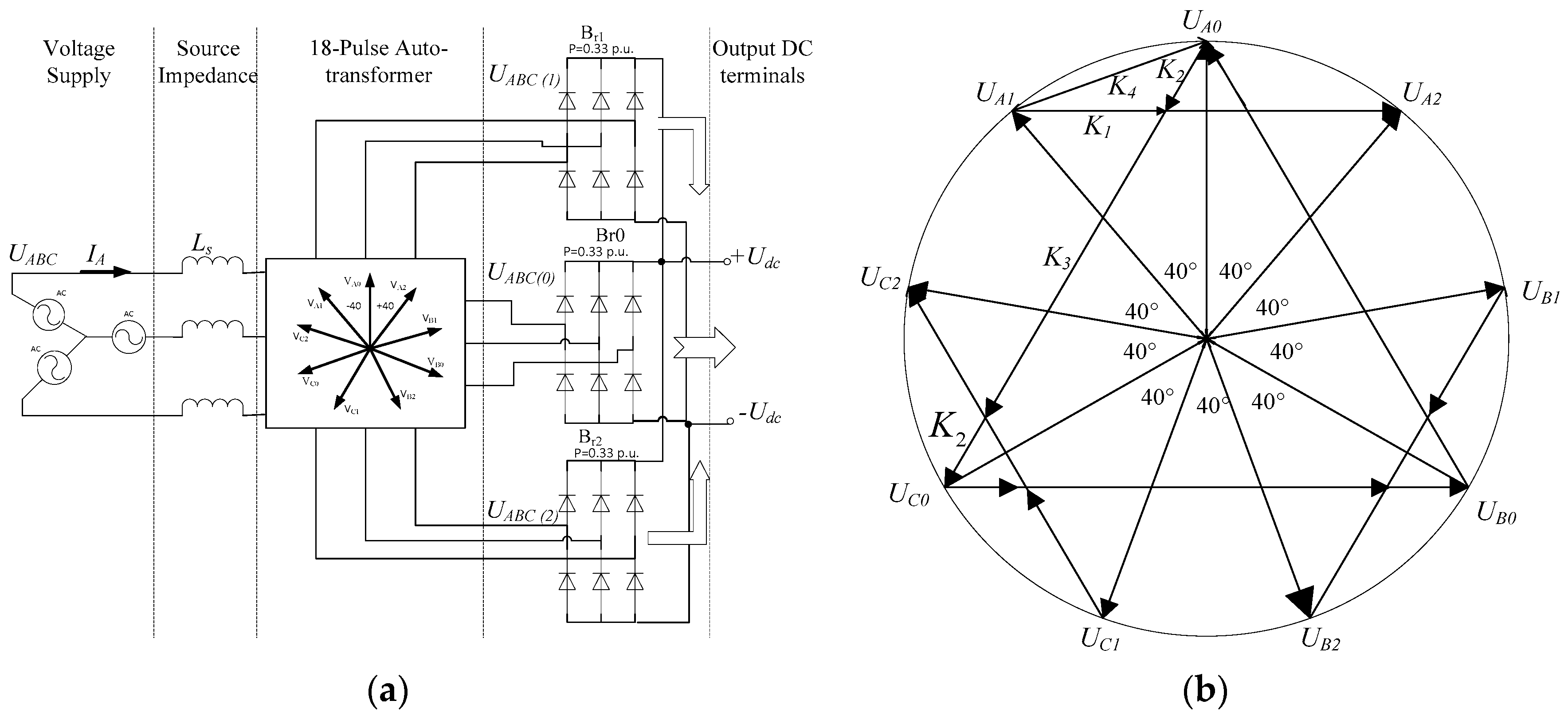
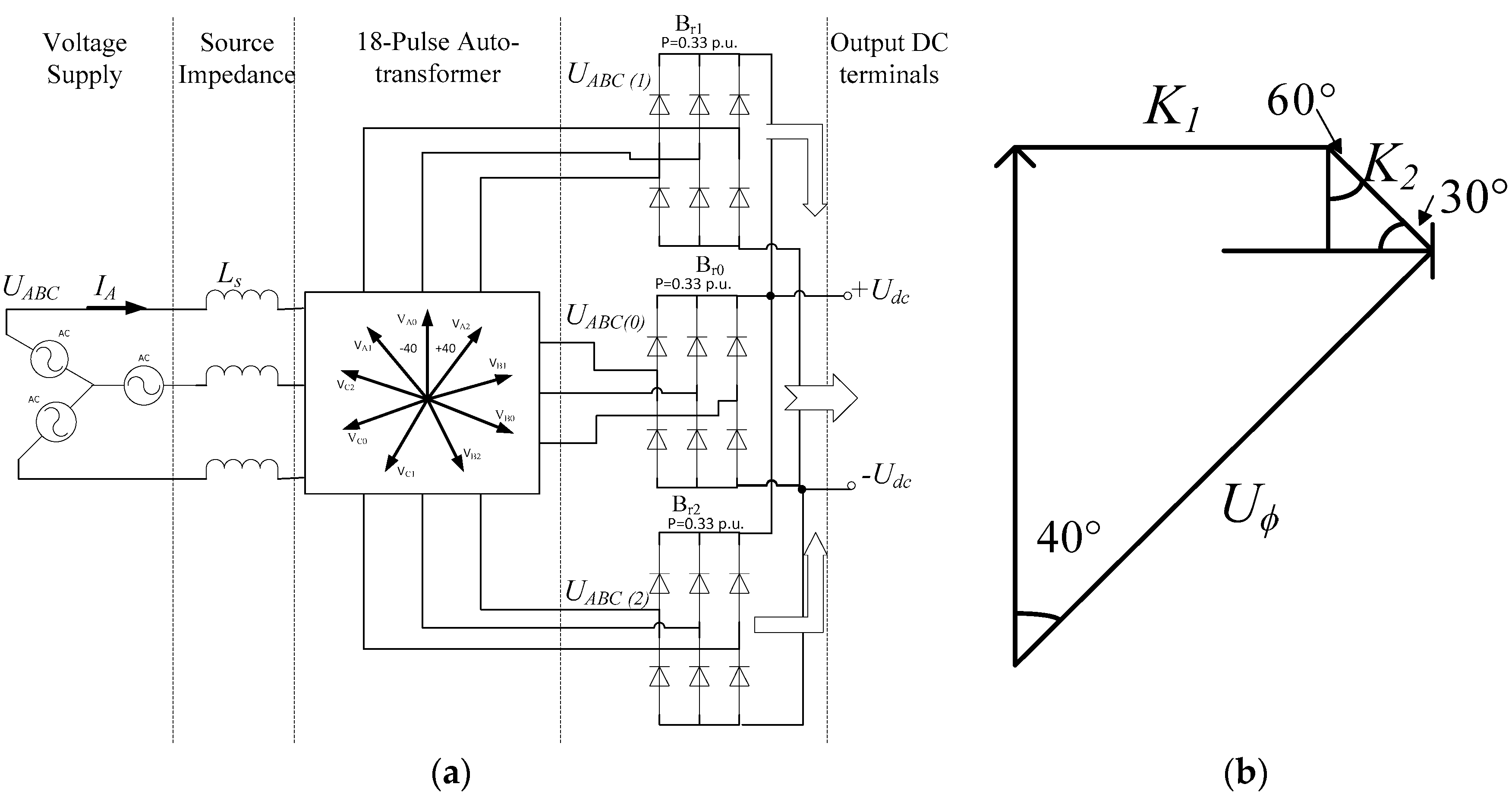
2. 18-Pulse ATRU Topologies
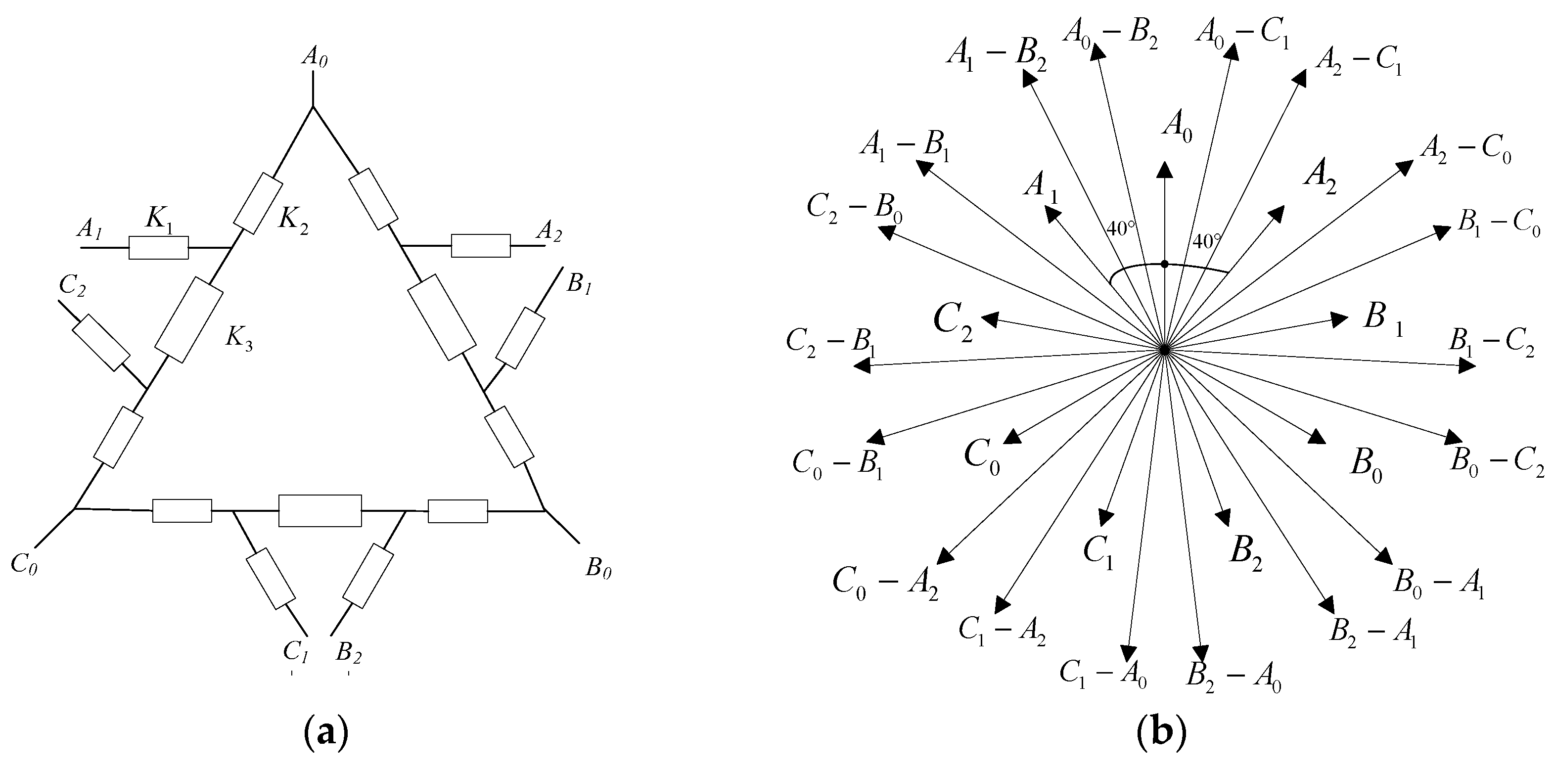
2.1. Scheme A: Symmertic 18-Pulse Differential Delta
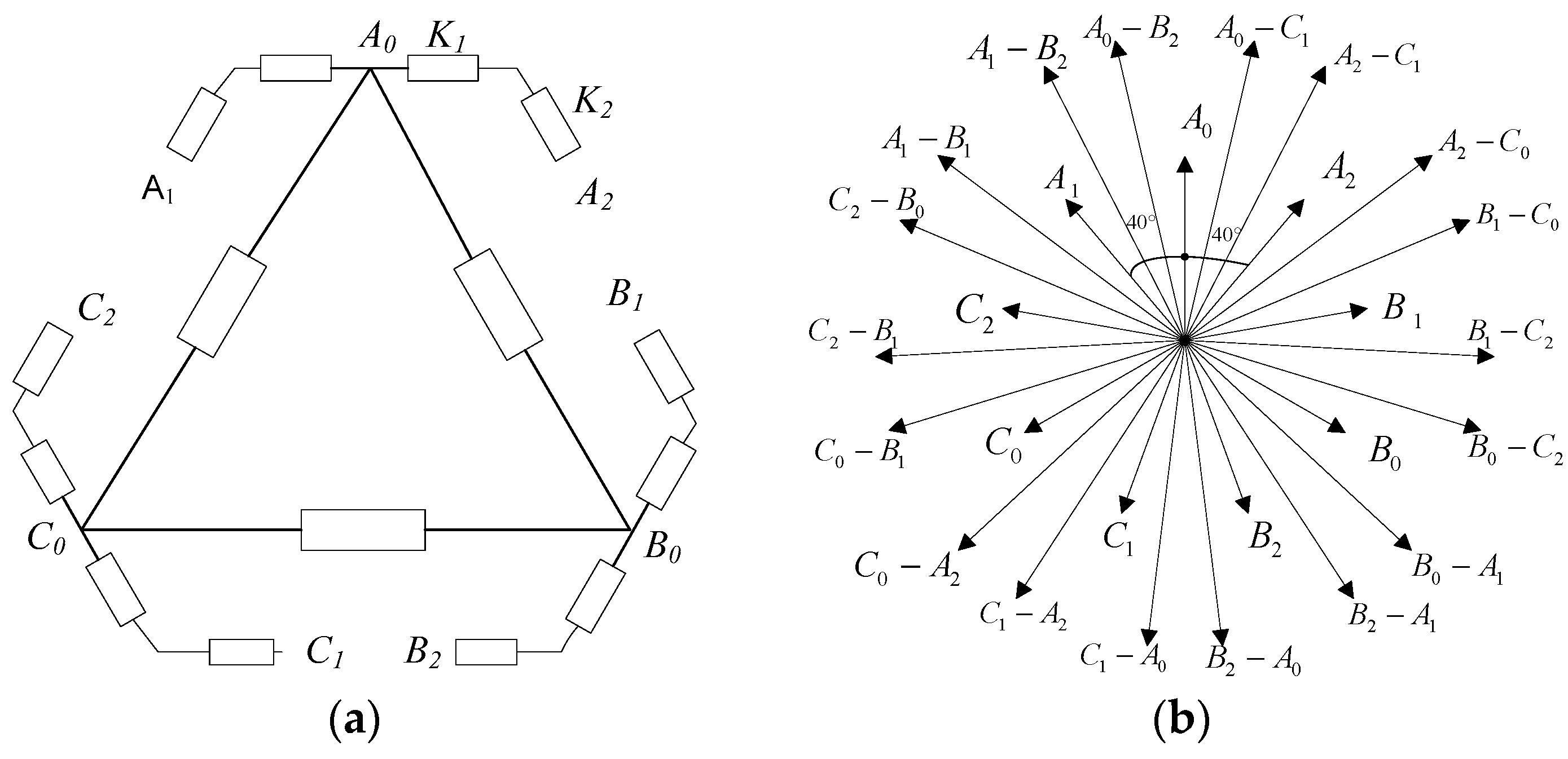
2.2. Scheme B: Symmertic 18-Pulse Differential T-Delta
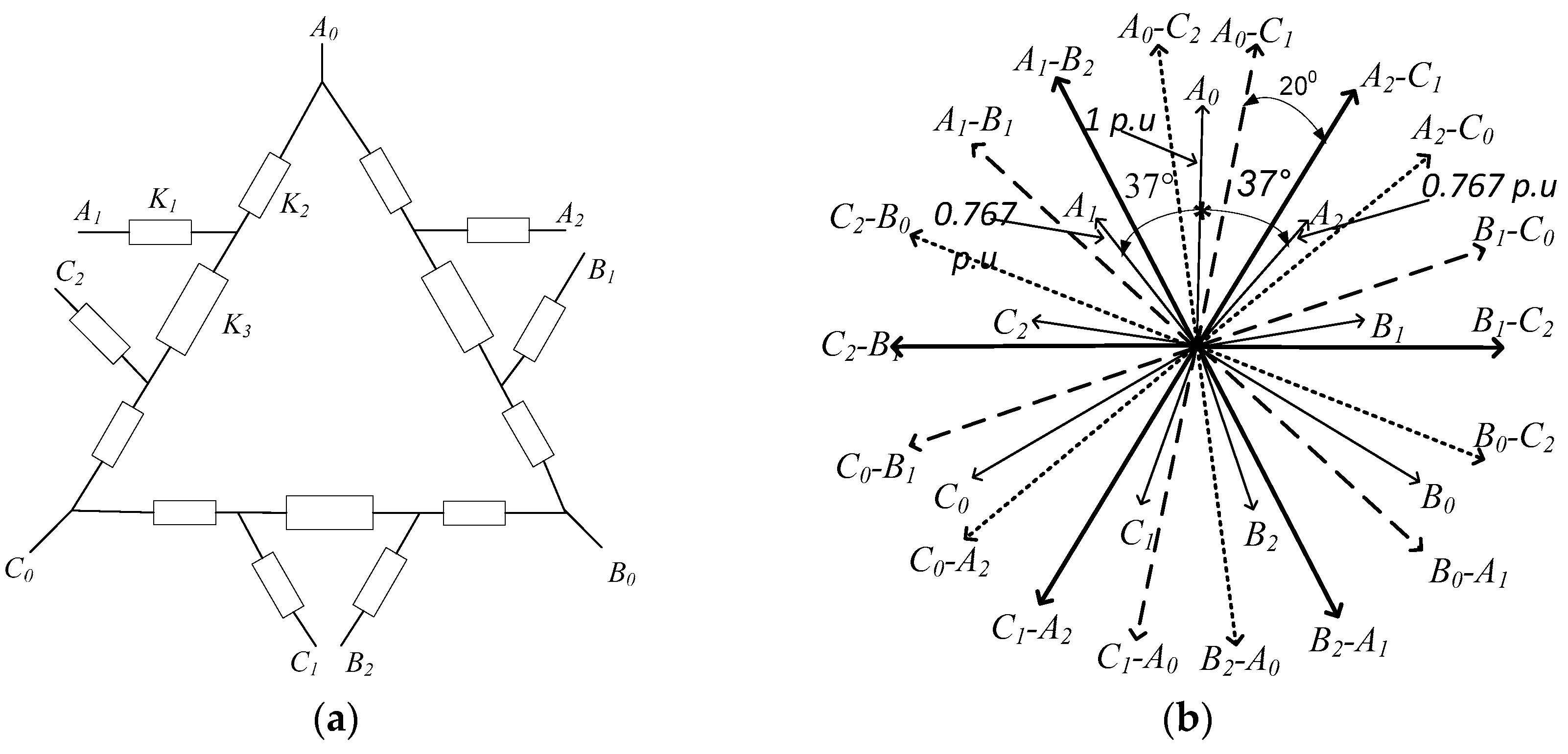
2.3. Scheme C: Asymmertic 18-Pulse Differential Delta
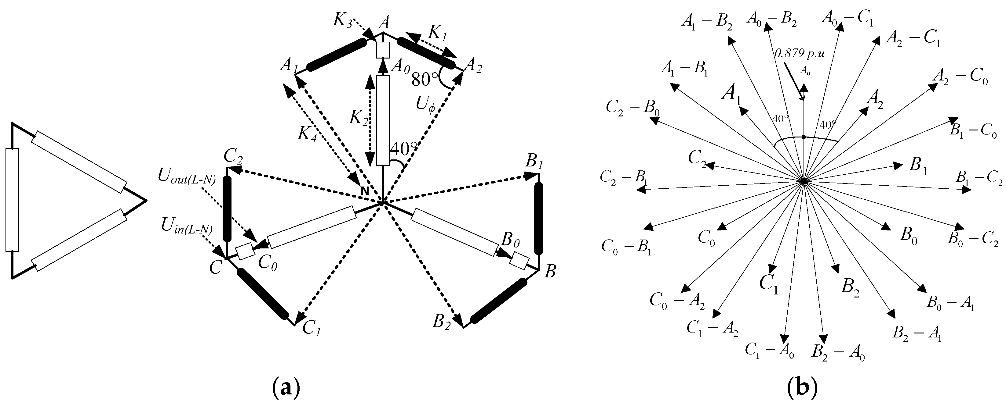
2.4. Scheme D: Symmertic Differential Fork
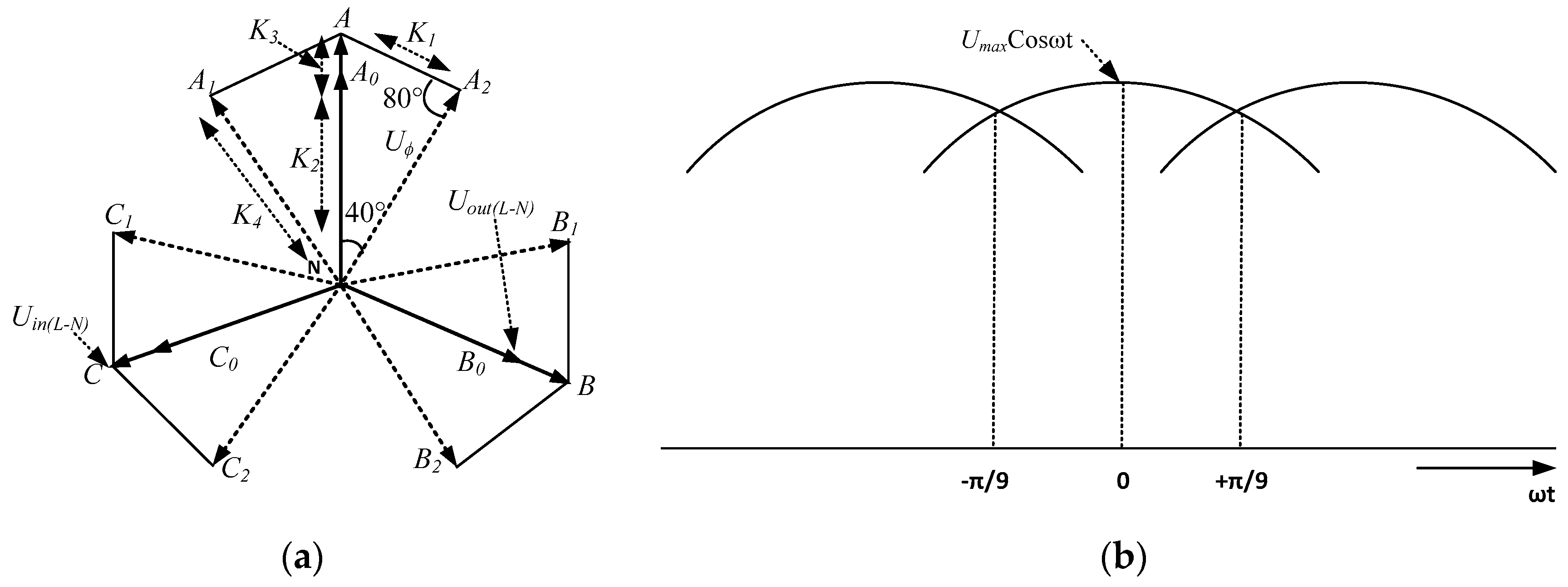
3. Voltages and Currents Analysis
3.1. Scheme A
3.2. Scheme B
3.3. Scheme C
3.4. Scheme D
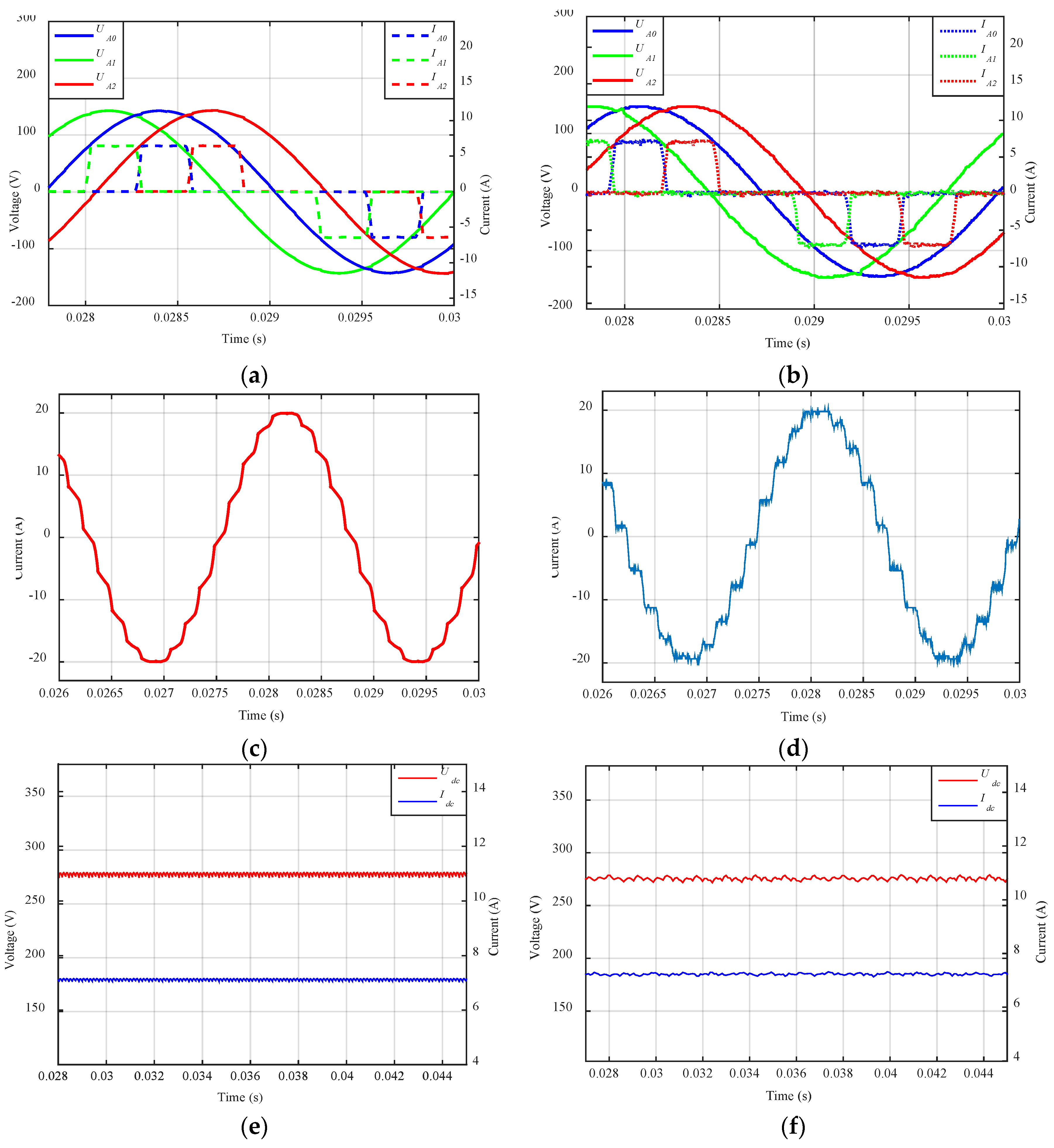
4. Simulation and Hardware Results
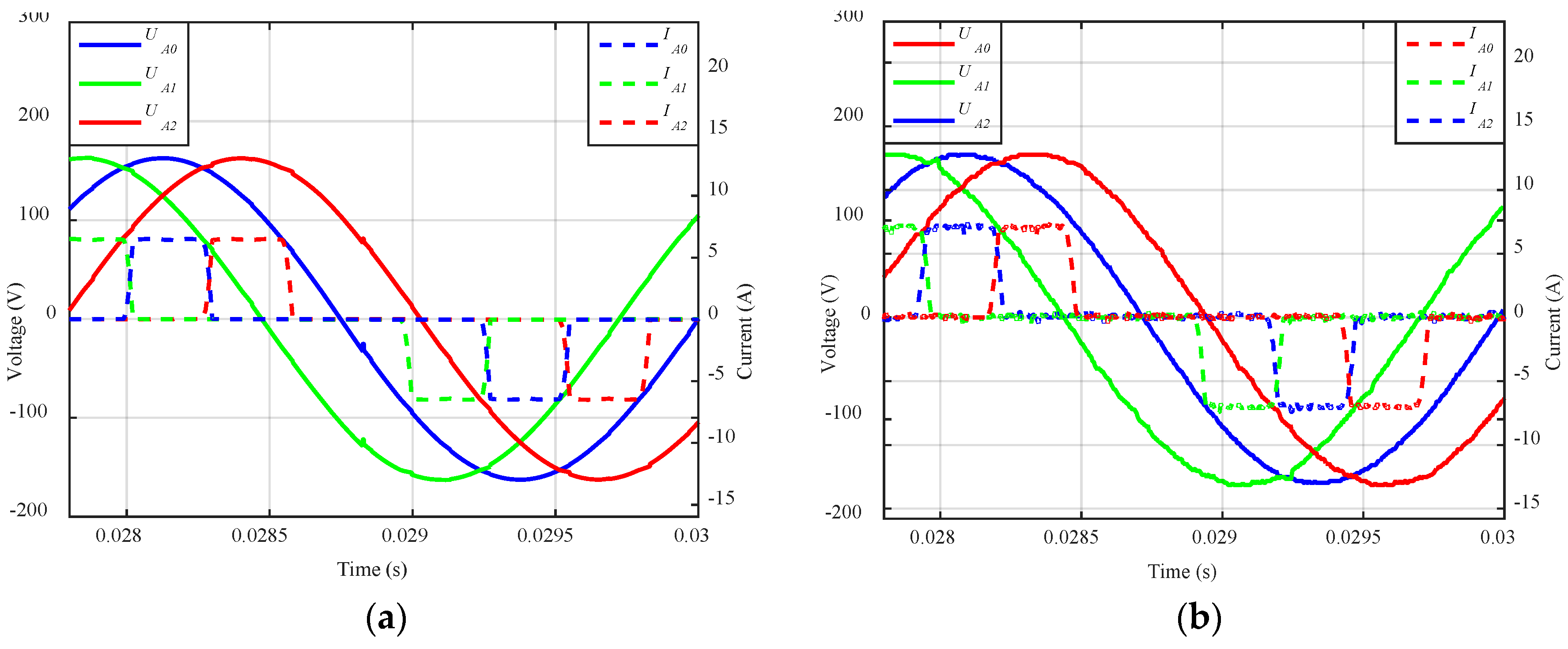
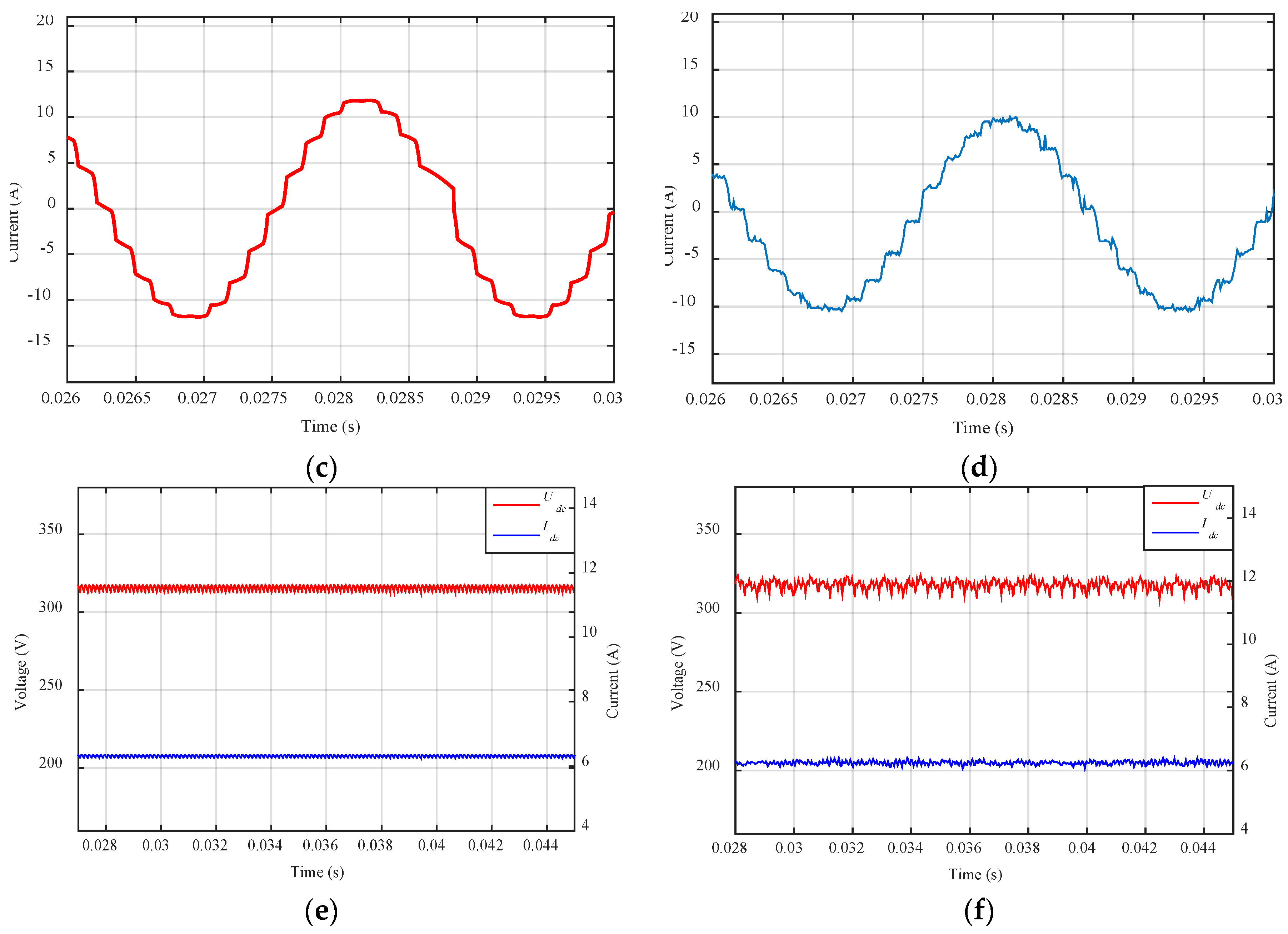
4.1. Scheme A
4.2. Scheme B
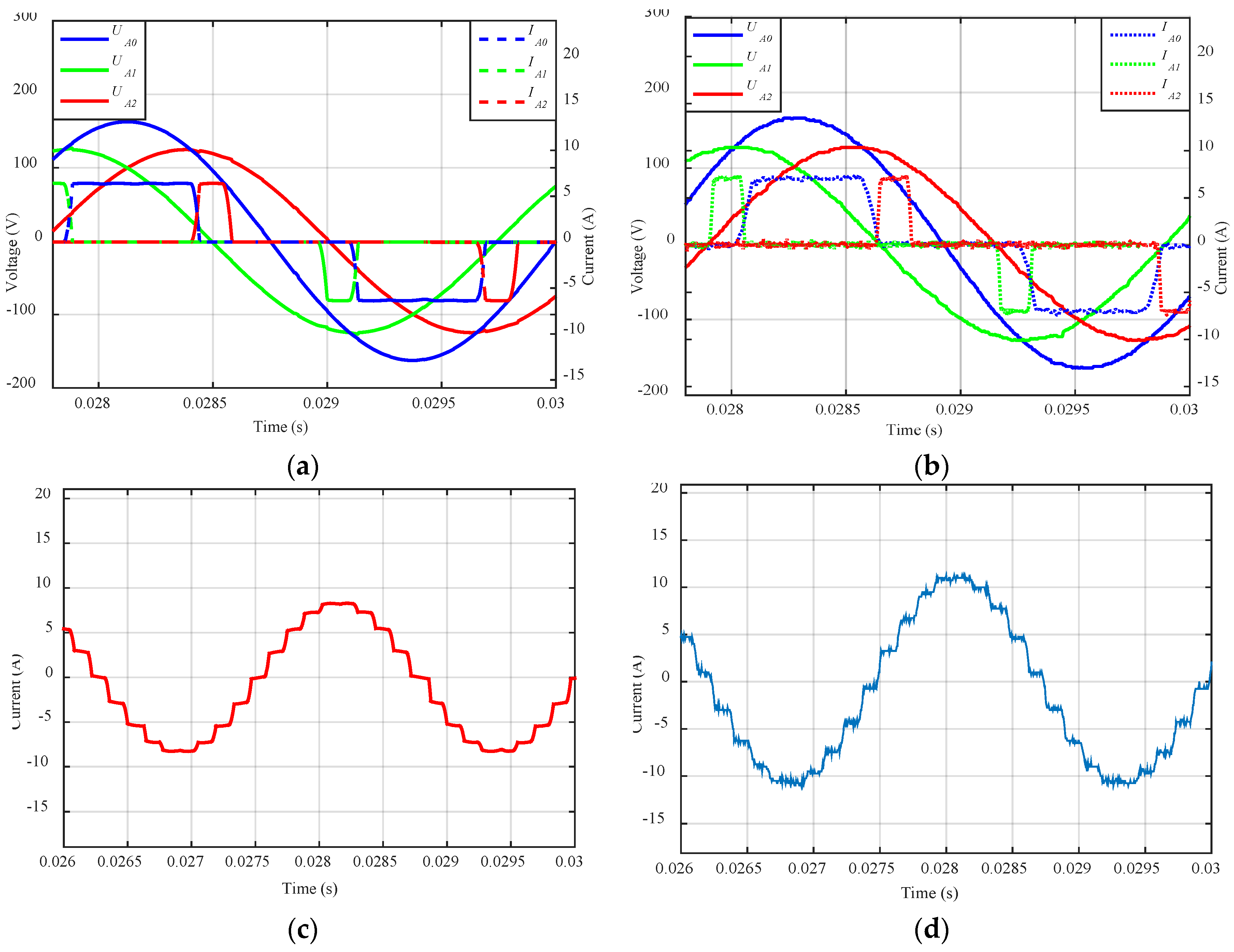
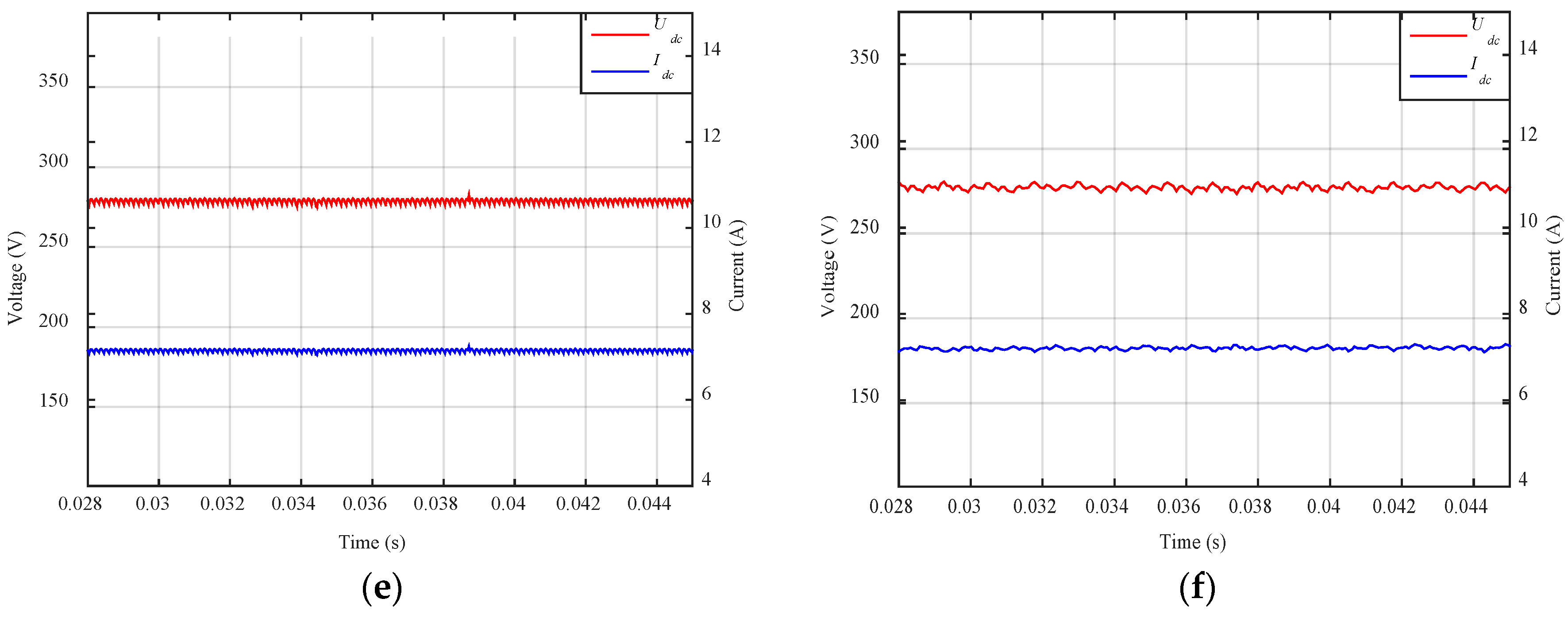
4.3. Scheme C
4.4. Scheme D
5. Conclusions
Author Contributions
Conflicts of Interest
References
- Kulkarni, A.; Chen, W.; Bazzi, A. Implementation of Rapid Prototyping Tools for Power Loss and Cost Minimization of DC-DC Converters. Energies 2016, 9, 509. [Google Scholar] [CrossRef]
- Aghighi, S.; Baghramian, A.; Atani, R.E. Averaged Value Analysis of 18-Pulse Rectifiers for Aerospace Applications. In Proceedings of the IEEE International Symposium on Industrial Electronics 2009, Seoul Olympic Parktel, Seoul, Korea, 5–8 July 2009. [Google Scholar]
- Kuo, M.; Tsou, M. Novel Frequency Swapping Technique for Conducted Electromagnetic Interference Suppression in Power Converter Applications. Energies 2017, 10, 24. [Google Scholar] [CrossRef]
- Li, W.; Liang, L.; Liu, W.; Wu, X. State of Charge Estimation of Lithium-Ion Batteries Using a Discrete-Time Nonlinear Observer. IEEE Trans. Ind. Electron. 2017, 64, 8557–8565. [Google Scholar] [CrossRef]
- Lei, T.; Wu, C.; Liu, X. Multi-Objective Optimization Control for the Aerospace Dual-Active Bridge Power Converter. Energies 2018, 11, 1168. [Google Scholar] [CrossRef]
- Henke, M.; Narjes, G.; Hoffmann, J.; Wohlers, C.; Urbanek, S.; Heister, C.; Steinbrink, J.; Canders, W.-R.; Ponick, B. Challenges and Opportunities of Very Light High-Performance Electric Drives for Aviation. Energies 2018, 11, 344. [Google Scholar] [CrossRef]
- Onambele, C.; Elsied, M.; Mpanda Mabwe, A.; El Hajjaji, A. Multi-Phase Modular Drive System: A Case Study in Electrical Aircraft Applications. Energies 2018, 11, 5. [Google Scholar] [CrossRef]
- Pickert, V.; Al-Mhana, T.; Atkinson, D.; Zahawi, B. Forced Commutated Controlled Series Capacitor Rectifier for More Electric Aircraft. IEEE Trans. Power Electron. 2018. [Google Scholar] [CrossRef]
- Chen, J.; Wang, C.; Chen, J. Investigation on the Selection of Electric Power System Architecture for Future More Electric Aircraft. IEEE Trans. Transp. Electrification 2018. [Google Scholar] [CrossRef]
- Nagel, N. Actuation Challenges in the More Electric Aircraft: Overcoming Hurdles in the Electrification of Actuation Systems. IEEE Electrification Mag. 2017, 4, 38–45. [Google Scholar] [CrossRef]
- Khan, S.; Zhang, X.; Khan, B.M.; Ali, H.; Zaman, H.; Saad, M. AC and DC Impedance Extraction for 3-Phase and 9-Phase Diode Rectifiers Utilizing Improved Average Mathematical Models. Energies 2018, 11, 550. [Google Scholar] [CrossRef]
- Swamy, M.; Kume, T.J.; Takada, N. A Hybrid 18-Pulse Rectification Scheme for Diode Front-End Rectifiers with Large DC-Bus Capacitor. IEEE Trans. Ind. Appl. 2010, 46, 2484–2494. [Google Scholar] [CrossRef]
- Burgos, R.; Uan-Zo-li, A.; Lacaux, F.; Wang, F.; Boroyevich, D. Analysis and Experimental Evaluation of Symmetric and Asymmetric 18-Pulse Autotransformer Rectifier Topologies. In Proceedings of the 2007 IEEE Power Conversion Conference—Nagoya (PCC ’07), Nagoya, Japan, 2–5 April 2007. [Google Scholar]
- Chiniforoosh, S.; Hamid, A.; Juri, J. A Generalized Methodology for Dynamic Average Modeling of High-Pulse-Count Rectifiers in Transient Simulation Programs. IEEE Trans. Energy Convers. 2016, 31, 228–239. [Google Scholar] [CrossRef]
- Meng, F.; Xu, X.; Gao, L. A Simple Harmonic Reduction Method in Multipulse Rectifier Using Passive Devices. IEEE Trans. Ind. Inform. 2017, 13, 2680–2692. [Google Scholar] [CrossRef]
- Mon-Nzongo, D.L.; Ipoum-Ngome, P.G.; Jin, T.; Song-Manguelle, J. An Improved Topology for Multipulse AC/DC Converters within HVDC and VFD Systems: Operation in Degraded Modes. IEEE Trans. Ind. Electron. 2018, 65, 3646–3656. [Google Scholar] [CrossRef]
- Paice, D.A. Power Electronic Converter Harmonic Multipulse Methods for Clean Power; IEEE Press: Piscataway, NJ, USA, 1996. [Google Scholar]
- Shahbaz, K.; Gao, Z.H.; Husan, A.; Kashif, H.; Izhar, U.H. Comparative analysis of differential delta configured 18-pulse ATRU. In Proceedings of the 2015 International Conference on Electrical Systems for Aircraft, Railway, Ship Propulsion and Road Vehicles (ESARS), Aachen, Germany, 3–5 March 2015. [Google Scholar]
- IEEE Recommended Practices and Requirements for Harmonic Control in Electrical Power Systems; IEEE Std. 519-1992; Institute of Electrical and Electronics Engineers, Inc.: New York, NY, USA, 1993.
- Kuniomi, O. Autotransformer-Based 18-Pulse Rectifiers without Using DC-Side Interphase Transformers: Classification and Comparison. In Proceedings of the International Symposium on Power Electronics, Electrical Drives, Automation and Motion (SPEEDAM 2008), Ischia, Italy, 11–13 June 2008. [Google Scholar]


| Characteristic Harmonics | 6-Pulse | 12-Pulse | 18-Pulse |
| 5th | - | - | |
| 7th | - | - | |
| 11th | 11th | - | |
| 13th | 13th | - | |
| 17th | - | 17th | |
| 19th | - | 19th | |
| 23rd | 23rd | - | |
| 25th | 25th | - | |
| 29th | - | - | |
| 31st | - | - | |
| 35th | 35th | 35th | |
| 37th | 37th | 37th |
| Scheme | Uin (RMS) | CT,eq | Lac (uH) | Ldc (mH) | Rdc (Ω) | K1 | K2 | K3 | Phase Shift Angle | Udc |
|---|---|---|---|---|---|---|---|---|---|---|
| A | 115 | 0.51 | 400 | 1 | 30 | 0.293 | 0.156 | 0.688 | 40° | 1.6 ULL |
| B | 115 | 0.58 | 300 | 1 | 30 | 0.293 | 0.156 | N.A. | 40° | 1.6 ULL |
| C | 115 | 0.31 | 1000 | 1 | 30 | 0.137 | 0.258 | 0.484 | 36.9° | 1.407 ULL |
| D | 115 | 0.68 | 10 | 1 | 30 | 0.653 | 0.879 | 0.1206 | 40° | 1.407 ULL |
| Percent (%) Harmonic Currents w.r.t Fundamental Harmonic | |||||||||
|---|---|---|---|---|---|---|---|---|---|
| Harmonic No. | Scheme A | Scheme B | Scheme C | Scheme D | Limits | ||||
| Sim | Meas | Sim | Meas | Sim | Meas | Sim | Meas | - | |
| 1 | 100 | 100 | 100 | 100 | 100 | 100 | 100 | 100 | - |
| 3 | 0.29 | 0.35 | 0.06 | 0.13 | 0.03 | 0.10 | 0.01 | 0.05 | 2 |
| 5 | 0.26 | 0.30 | 0.18 | 0.24 | 0.14 | 0.25 | 0.18 | 0.20 | 2 |
| 7 | 0.20 | 0.21 | 0.05 | 0.11 | 0.10 | 0.15 | 0.06 | 0.10 | 2 |
| 9 | 0.03 | 0.01 | 0.06 | 0.03 | 0.04 | 0.30 | 0.00 | 0.02 | 1.11 |
| 11 | 0.21 | 0.15 | 0.02 | 0.07 | 0.15 | 0.01 | 0.09 | 0.15 | 3 |
| 13 | 0.07 | 0.12 | 0.09 | 0.14 | 0.09 | 0.20 | 0.14 | 0.19 | 3 |
| 15 | 0.15 | 0.19 | 0.06 | 0.09 | 0.01 | 0.11 | 0.00 | 0.03 | 3 |
| 17 | 2.95 | 3.10 | 2.85 | 2.99 | 1.76 | 3.01 | 2.88 | 3.00 | 4 |
| 19 | 2.13 | 2.18 | 2.09 | 2.10 | 1.29 | 1.98 | 2.28 | 2.56 | 4 |
| THD | 3.82 | 3.95 | 3.61 | 3.91 | 2.27 | 3.55 | 3.90 | 3.98 | - |
© 2018 by the authors. Licensee MDPI, Basel, Switzerland. This article is an open access article distributed under the terms and conditions of the Creative Commons Attribution (CC BY) license (http://creativecommons.org/licenses/by/4.0/).
Share and Cite
Khan, S.; Zhang, X.; Saad, M.; Ali, H.; Muhammad Khan, B.; Zaman, H. Comparative Analysis of 18-Pulse Autotransformer Rectifier Unit Topologies with Intrinsic Harmonic Current Cancellation. Energies 2018, 11, 1347. https://doi.org/10.3390/en11061347
Khan S, Zhang X, Saad M, Ali H, Muhammad Khan B, Zaman H. Comparative Analysis of 18-Pulse Autotransformer Rectifier Unit Topologies with Intrinsic Harmonic Current Cancellation. Energies. 2018; 11(6):1347. https://doi.org/10.3390/en11061347
Chicago/Turabian StyleKhan, Shahbaz, Xiaobin Zhang, Muhammad Saad, Husan Ali, Bakht Muhammad Khan, and Haider Zaman. 2018. "Comparative Analysis of 18-Pulse Autotransformer Rectifier Unit Topologies with Intrinsic Harmonic Current Cancellation" Energies 11, no. 6: 1347. https://doi.org/10.3390/en11061347
APA StyleKhan, S., Zhang, X., Saad, M., Ali, H., Muhammad Khan, B., & Zaman, H. (2018). Comparative Analysis of 18-Pulse Autotransformer Rectifier Unit Topologies with Intrinsic Harmonic Current Cancellation. Energies, 11(6), 1347. https://doi.org/10.3390/en11061347