Optimal Scheduling Strategies of Distributed Energy Storage Aggregator in Energy and Reserve Markets Considering Wind Power Uncertainties

Abstract

With continuous technological improvement and economic development of energy storage, distributed energy storage (DES) will be widely connected to the distribution network. If fragmented DES systems are aggregated to form a distributed energy storage aggregator (DESA), the DESA will have great potential to participate in the day-ahead energy and reserve market and the balancing market. The DESA could act as a mediator between the market and DES consumers, enabling beneficial coordination for DES owners and power systems. This paper presents a bilevel optimization model for DESAs in the energy and reserve market under wind power uncertainties. In the lower-level problem, generating companies, wind power plants (WPP), and DESAs are optimized for scheduling day-ahead (DA) energy and the reserve market. In the upper-level problem, operational strategies for DES systems and DESAs are designed to deal with wind power uncertainties in the balancing market. The DESA splits its resources between the energy and reserve markets so that it can reduce total power system consumption, and mutual profit for the system and end customers is achieved. This model is formulated as a mixed-integer linear programming (MILP) program, which can be solved with commercial software. The validity of the bilevel optimization model is verified by the eight-node test transmission system and IEEE-33 bus distribution system.

1. Introduction

With the increase of electric vehicles and distributed power generation (distributed photovoltaic, wind power generation, combined heat-cold power units) connected to the distribution network, the distribution system operator (DSO) needs more high-quality demand-side resources. These resources can respond quickly and be controlled in real time against the undesirable impact of distributed resources [1,2], such as speed generation variation and load variation. In addition, future power systems with high penetration of variable renewables will require more flexible generation and demand-side resources in order to maintain secure and stable operation. The distributed energy storage (DES) system is a fast-response and bidirectional adjustment demand-side resource. It reduces energy and peak network costs for DSOs and significantly improves the reliability of the distribution network. With continuous and advanced construction of active distribution networks (ADNs) [3], access for a large number of DES systems to distribution networks has become an inevitable trend [4]. However, the individual participation of DES systems at the system level would not be possible for two reasons: (1) their individual capacity is below the required minimum to participate in the day-ahead (DA) market and balancing market, and (2) the scheduling organization cannot easily obtain DES systems’ aggregation information and it would be difficult to manage. The distributed energy storage aggregator (DESA) [5] adopts advanced communication and control technologies to aggregate and control DES systems in the distribution network. In this way, it can form a large-energy and high-power schedulable resource pool. This resource pool could provide reserve capacity and participate in the energy market on multiple time scales, and the DESA is helpful for quickly maintaining the stability of system frequency, voltage, and the rest of ancillary services.

DESAs will play an important role in the power system. They do not replace existing components of the electricity value chain but rather allow the existing ones to do their job better and cheaper [6]. On the one hand, the optimized operation of DES systems mainly enables them to provide voltage support, reduce distribution losses, increase capacity support, buffer variable wind and solar energy, and reduce expansion investment in the distribution network [7]. On the other hand, DESAs have the advantages of reducing transmission congestion, curtailing renewable energy, and deferring transmission in investment for transmission system operators (TSOs). Moreover, DESAs could play an important role in price arbitrage, fast regulation, spinning reserve, power quality, and black start for independent system operators (ISOs). DESA represents a new tool (management strategies, control and optimization algorithms), which is valuable for guaranteeing system stability, reducing system cost, and increasing customer profit. The focus of this paper is to define the features of the DESA and model its strategic behavior in the wholesale market considering wind power uncertainties. In this paper, DESA is designed as a flexibility manager and a balance responsible party.

A good overview on the planning and operation of DES in a distribution network can be found in [8,9]. In [10], a new method for optimal integration of DES at minimum cost is proposed. The optimal method allows DES to provide voltage support, delay network upgrade, and offer aggregation resources to TSOs. In [11], an algorithm and optimization participation strategies are presented that allow aggregators to cooperatively control such DES systems in accordance with electricity market rules and interactive strategies. In [12], a comprehensive planning framework for ascertaining the most cost-effective siting and sizing of DES to maximize the benefits in the distribution network is designed. A strategy for optimal integration of DES systems to improve the load hosting ability is presented in [13]. The strategy model considered two primary factors—Distribution Network Operator (DNO) cost and DES cycling cost—to offer three services—voltage regulation, peak shaving, and loss reduction. In [14], a comprehensive optimal allocation model of DES considering operation strategy is presented. The problems of optimal capacity and sizing of DES are solved by minimum cost of DES operation and investment. In [15], an effective method is proposed that allocate DES systems for spinning reserve or frequency regulation to improve system reliability.

Research on interactive modes and operational strategies of different types of aggregators to participate in the electricity market and ancillary services have also been proposed in the literature. A bidding strategy is proposed in [16] for electric vehicle (EV) aggregators to maximize their profits by trading energy and regulation reserves in the electricity market. The EV aggregator is the required mediator between a large number of EVs and power system operators and could provide some services to power systems. Thermostatically controlled load (TCL) aggregators are introduced in [17,18]. They could provide load following services and regulation reserves in the power system. In [19], a day-ahead dispatch framework for virtual power plants (VPPs) in joint energy and regulation reserve market considering the penalty cost of CO₂ emissions is presented. In [20], a cost model of load curtailment for different services is proposed, allowing the demand response aggregator and generation company to participate in/schedule the energy and reserve (ancillary) market. A bilevel optimization model of distribution companies in the wholesale reserve market is proposed in [21]. In the proposed model, the distribution company and independent system operator are modeled in the lower-level and upper-level problem, respectively. Energy storage systems (ESSs) that integrate renewable energy resources to provide arbitrage and ancillary services are introduced in [22,23,24]. ESSs can participate in both the energy and reserve markets, because they can reduce power system operation cost and improve system stability. These different types of aggregators are able to purchase cheaper energy, provide ancillary services more economically, and reduce carbon more effectively than traditional generation sources.

The DES solutions and emerging aggregators mentioned above are being increasingly applied in the energy and reserve markets. Therefore, it is an excellent opportunity for DESAs to aggregate and manage DES systems. DESAs would participate in the energy market by earning energy arbitrage, providing reserve capacity in the reserve market, and dealing with uncertainties in the balancing market. In the power system, system reserves are used to maintain stability and reduce wind power curtailment to minimize the operation costs of systems and low carbon emissions. The major contributions of this paper are as follows: (1) We propose a new bilevel optimization model for DESAs taking part in the day-ahead energy and reserve markets and the balancing market; (2) we establish an effective and extensible model of DESA aggregation considering the operational constraints of DES in distribution network; and (3) we contrast optimal strategies of DESA in different uncertain scenarios with wind power participation.

The remainder of the paper is organized as follows: The problem is described in Section 2, and Section 3 describes the mathematical formulation of the proposed approach. Section 4 provides a description of the test scenarios and an analysis of simulation results. Finally, conclusions on the application of the integrated approach and future work are shown in Section 5.

2. Problem and Method Statement

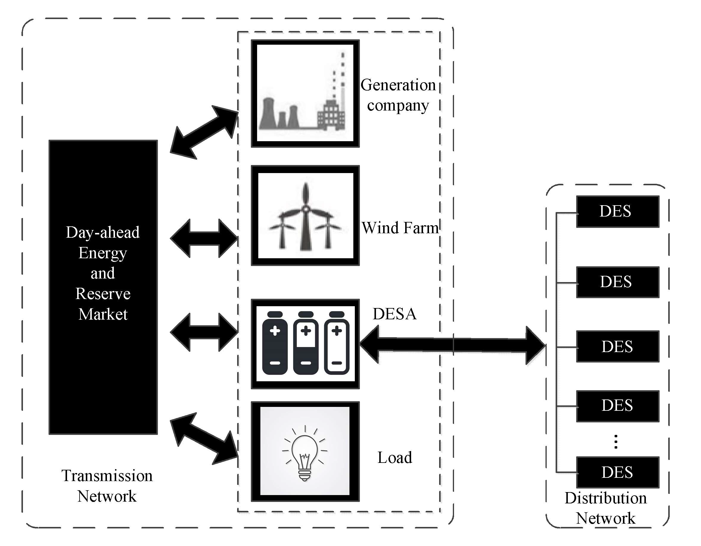
2.1. Problem Description

In this paper, the optimal strategy of a DESA in the day-ahead energy and reserve markets is described as a bilevel problem. The DESA participates in the energy market as a price-taker. Figure 1 shows the framework of the bilevel problem. Traditional DES systems could only make a profit through energy arbitrage in the energy market. This paper presents a new business model and operation strategy through the DESA. The operation strategy of DESAs and DES systems is modeled in the upper-level problem. In the upper-level problem, the aim of the DESA is to maximize its economic profit. The DESA aggregates DES systems in the distribution network to form a schedulable capacity energy resource pool. The DESA purchases/sells energy from the DA market and provides reserve services. The DESA earns a portion through electricity price arbitrage, providing spinning reserve and dealing with wind power uncertainties in the balancing market. In the lower-level problem, the generation companies, the wind power plants, the DESA, and loads are the participants of the day-ahead energy and reserve markets. We assume that generation companies and wind power plants have the same stakeholders. The operational objective of the lower-level problem is to minimize the operating expense of the generation companies and maximize social welfare. Thus wind power curtailment could be decreased. Due to the uncertainty and variability of wind power output, there is uncertain error between predicted output and actual output. Therefore, it is necessary to provide a corresponding proportion of spinning reserves in the day-ahead dispatch plan in order to decrease wind power curtailment. DES systems are demand-side resources that respond quickly and flexibly, so they could respond to fluctuations of wind power output error in real time. Finally, the DESA would provide an optimal scheduling scheme for DES systems in order to minimize the generation companies’ energy cost and maximize profit.

The DESA is assumed as a link in the bilevel problem. The decision variables of the upper-level problem are the charging and discharging power plan of DES systems, providing a reserve plan of DES. The decision variables of the lower-level problem are power output of generators, reserves provided by generators, sell/purchase energy by the DESA in/from energy market, and reserves provided by the DESA. In each layer, there are decision variables that link the upper and lower stages. After solving the lower-level problem, the variables consist of the DESA sell/purchase energy in/from the day-ahead energy market, providing reserves in the reserve market. They are passed to upper-level problem as parameters. In the upper-level problem, the operational constraints of the DESA consist of the DES operational configuration. They are passed to the lower-level problem as parameters.

2.2. System Uncertainly Analysis

In the power system, wind power output is affected by many factors. In this way, wind power output has uncertainty. Therefore, wind power output is usually predicted to solve this problem. However, there is always a prediction error between predictive and actual value. The relationship between the two values can be calculated by Equation (1).

$$P_{t,w}^{Forecast}+{\xi }_w^t=P_{t,w,s}^{WPP}$$

(1)

where $P_{t,w}^{Forecast}$ is the predictive value of wind power output at time t, ${\xi }_w^t$ is the prediction error at time t, and $P_{t,w,s}^{WPP}$ is the actual value of wind power output at time t.

In order to accurately describe the prediction error, this paper utilizes the Monte Carlo model to generate wind power output scenarios. The Monte Carlo model is based on probability and mathematical statistics and has the advantage of solving problems with uncertainty. The research shows that the prediction error of the output of renewable energy and fluctuating load can be approximately assumed to be normally distributed with a mean value of 0 in a certain time frame [25]. Therefore, the prediction error should meet Equation (2). The standardized standard deviation (the wind farm installed capacity is used as the reference capacity in the standardization) can be expressed as Equation (3) [26]. It should be noted that the value of $\sigma$ is between 0 and 1. It is similar to per-unit value in the power system. However, known value is always required in scenario analysis. The conversion from per-unit value to known value should meet Equation (4). If $P_{\mathrm{wpre}}^t$ is the predicted wind power output (known value) at time t, moment ${\sigma }_w^t$ should meet Equation (5). Therefore, the prediction error should be normally distributed according to Equation (6). According to Equations (1) and (6), a number of wind power output scenarios can be generated with the Monte Carlo model.

$${\xi }_w^t\sim N\left(0,{\sigma }_w^t\right)$$

(2)

$$\sigma =0.02+0.2\times {\omega }_t$$

(3)

$${\sigma }_w^t=\sigma \times P_{WN}$$

(4)

$${\sigma }_w^t=0.2P_{\mathrm{wpre}}^t+0.02P_{WN}$$

(5)

$${\xi }_w^t\sim N\left(0,0.2P_{\mathrm{wpre}}^t+0.02P_{WN}\right)$$

(6)

where $\sigma$ is the standardized standard deviation, ${\omega }_t$ is the standardized wind power prediction output, ${\sigma }_w^t$ is the standard deviation at time t, and $P_{WN}$ is the wind farm installed capacity.

2.3. Scenario Reduction Strategy

Theoretically, if the scenarios generated by the Monte Carlo method are abundant, the probability of obtaining exact results of stochastic problems will be high. However, it will cost much computation time and increase complexity. Reducing large-scale scenarios needs to reduce computational cost but ensure that the reduced scenarios are approximate to the original scenarios. Fuzzy C-means clustering (FCMC) is a kind of clustering analysis that has high efficiency for calculating large datasets, and its time complexity is only about the first power of time.

When using FCMC to reduce scenarios, we need to give the number of clustering categories, set the iterative convergence conditions, and initialize each clustering center. It is assumed that the dataset is $X=\left\{x_1,x_2,\mathrm{...},x_n\right\}$; k is the number of clustering categories, $m_j\left(j=1,2,\mathrm{...},k\right)$ are clustering centers, and ${\mu }_j\left(x_i\right)$ is the member function that the sample i is subordinate to category $j$. In this way, the clustering loss function can be expressed by Equation (7). If the partial derivative of $J_f$ with respect to ${\mathrm{m}}_j$ and ${\mu }_j\left({\mathrm{x}}_i\right)$ is 0, the essential condition of obtaining the minimum for Equation (7) will meet Equations (8) and (9).

$$J_f={\displaystyle \sum _{j=1}^k{{\displaystyle \sum _{i=1}^n\left[{\mu }_j\left(x_i\right)\right]}}^b{\Vert x_i-m_j\Vert }^2}$$

(7)

$$m_j=\frac{{{\displaystyle \sum _{i=1}^n\left[{\mu }_j\left(x_i\right)\right]}}^b{x}_i}{{{\displaystyle \sum _{i=1}^n\left[{\mu }_j\left(x_i\right)\right]}}^b}$$

(8)

$${\mu }_j\left(x_i\right)=\frac{{\Vert x_i-m_j\Vert }^{-2/\left(b-1\right)}}{{\displaystyle \sum _{s=1}^k{\Vert x_i-m_s\Vert }^{-2/\left(b-1\right)}}}$$

(9)

where b is the weighted index. It is also called the smooth factor, and it can control shared degrees of patterns among fuzzy categories.

The membership function can be calculated by Equation (9) by current clustering centers, and the center of each clustering category can be recalculated by Equation (8) by the calculated membership function. These are iterated circularly until the convergence condition is satisfied. Then, the optimal solution is obtained. After all the clustering centers in the optimal solution are connected in a time series, a reduction of k scenarios is obtained. This will achieve the purpose of scenario reduction.

3. Mathematical Modeling

3.1. Modeling DESA

In this paper, the aggregation model of the DESA is described in Equations (10)–(13). Equations (10) and (11) are used to model the aggregation charging and discharging power of the DESA, respectively. Equation (12) is defined to present the aggregation energy storage of the DESA. The aggregation output limit of the maximum charging and discharging power of the DESA is described by Equation (13). The operation constraints of the DESA are described in the lower-level and upper-level problem.

$$P_t^{DESA,ch}={\displaystyle \sum _d(P_{t,d}^{DES,ch}-P_{t,d}^{DES,dis})}$$

(10)

$$P_t^{DESA,dis}={\displaystyle \sum _d(P_{t,d}^{DES,dis}-P_{t,d}^{DES,ch})}$$

(11)

$$E_t^{DESA}={\displaystyle \sum _d{E}_{t,d}^{DES}}$$

(12)

$${\overline{P}}_t^{DESA,ch/dis}={\displaystyle \sum _d{\overline{P}}_{t,d}^{DES}}$$

(13)

3.2. Modeling in the Lower-Level Problem

3.2.1. Objective Function

In the lower-level problem, the generation companies, wind power plants, and DESA participate in the day-ahead energy and reserve market simultaneously. The generation companies are considered as smart players that decrease operation cost by maximizing the consumption of wind power as much as possible. The generation companies can meet the energy demand and take part in the reserve market to guarantee system adequacy in case of contingency. Equation (14) represents the objective function of minimizing operational costs of the generation companies considering unit operating costs, the profit of the unit providing reserve, and the unit’s CO₂ emissions penalty during the time period.

$$\begin{array}{c}\min C(X^f)={\displaystyle \sum _{t\in T}[}{\displaystyle \sum _{g\in G}(}{C}_{t,g}^G{P}_{t,g}+C_{t,g}^f{b}_{t,g}+Sd{c}_g{z}_{t,g}+Su{c}_g{y}_{t,g}+C_{t,g}^{res,up}{r}_{t,g}^{up}+C_{t,g}^{res,dn}{r}_{t,g}^{dn}\\ -{\rho }_t^{res,up,DA}{r}_{t,g}^{up}-{\rho }_t^{res,down,DA}{r}_{t,g}^{dn}+P_{t,g}C{O}_2^{Unit}{\rho }^{C{O}_2})]\end{array}$$

(14)

3.2.2. Energy and Reserve Balance Constrains

Equations (15) and (16) are used to model the day-ahead energy and reserve balance constraints of system operation. In this paper, only the uncertainty of wind power is considered. Demand-side reserve power can be provided by generators and the DESA in the reserve market, and it can be used to stabilize the uncertainty and variability of wind power output.

$${\displaystyle \sum _{i\in I}{L}_{i,t}}+{\displaystyle \sum _{a\in A}{P}_t^{DESA,ch}}={\displaystyle \sum _{a\in A}{P}_t^{DESA,dis}}+{\displaystyle \sum _{g\in G}{P}_{t,g}^{}}+{\displaystyle \sum _{w\in W}{P}_{t,w}^{WPP}}$$

(15)

$$r_t^{DA}={\displaystyle \sum _{g\in G}(r_{t,g}^{up}-r_{t,g}^{dn})}+{\displaystyle \sum _{a\in A}}(r_{t,a}^{dis}-r_{t,a}^{ch})$$

(16)

3.2.3. Generator and WPP Operating Constrains

The output of the day-ahead energy and reserves provided by generators is strictly limited to the controllable range, as described by Equations (17) and (18). The minimum up- and down-time limit of generators is modeled in Equations (19) and (20). The unit commitment logic constraints are presented in Equations (21) and (22). Equation (21) describes the start-up and shut-down status change logic. Equation (22) enforces that the generator cannot start up and shut down at the same time. The ramp-up and -down limits of units are described in Equations (23) and (24). The spinning up and down reserve limits are defined by Equations (25) and (26). Equation (27) limits the scheduled wind power output.

Generator generation plus reserve limit is

$$P_{t,g}^{}+r_{t,g}^{up}\le {\overline{P}}_g^{}{b}_{t,g}$$

(17)

$$P_{t,g}^{}-r_{t,g}^{dn}\ge {\underset{\_}{P}}_g^{}{b}_{t,g}$$

(18)

Generator minimum up- and down-time constraints are

$${\displaystyle {\sum }_{h=t-U{t}_g+1}^t{y}_{h,g}\le b_{t,g}}$$

(19)

$${\displaystyle {\sum }_{h=t-D{t}_g+1}^t{z}_{h,g}\le 1-b_{t,g}}$$

(20)

Unit commitment logic constraints are

$$y_{t,g}-z_{t,g}=b_{t,g}-b_{t-1,g}$$

(21)

$$y_{t,g}+z_{t,g}\le 1$$

(22)

Ramp-up and -down limits are

$$P_{t,g}^{}-P_{t-1,g}^{}\le R{u}_g$$

(23)

$$P_{t-1,g}^{}-P_{t,g}^{}\le R{d}_g$$

(24)

Generator side reserve limits are

$$0\le r_{t,g}^{up}\le {\overline{r}}_g^{up}$$

(25)

$$0\le r_{t,g}^{dn}\le {\overline{r}}_g^{dn}$$

(26)

WPP constraints are

$$0\le P_{t,w}^{WPP}\le {\overline{P}}_{t,w}^{WPP}$$

(27)

3.2.4. DESA Constraints

The operational constraints of the DESA are presented in Equations (28)–(36). The minimum and maximum limits of DESA charging power, discharging power, and energy are described by Equations (28)–(31), respectively. The energy and power limitations of the DESA to provide energy and reserves are presented in Equations (32) and (33), respectively. DESA energy balance is presented in Equation (34). The relationships between charging/discharging reserve and energy capacity of the DESA are described in Equations (35) and (36).

$$0\le P_t^{DESA,dis}\le {\overline{P}}_a^{DESA,dis}$$

(28)

$$0\le P_t^{DESA,ch}\le {\overline{P}}_a^{DESA,ch}$$

(29)

$$0\le r_{t,a}^{dis}\le R_a^{dis}$$

(30)

$$0\le r_{t,a}^{ch}\le R_a^{ch}$$

(31)

$$0\le P_{t,a}^{DESA,dis}+r_{t,a}^{dis}\le {\overline{P}}_a^{DESA,dis}$$

(32)

$$0\le P_{t,a}^{DESA,ch}+r_{t,a}^{ch}\le {\overline{P}}_a^{DESA,ch}$$

(33)

$$E_t^{DESA}=E_{t-1}^{DESA}+P_{t-1}^{DESA,ch}-P_{t-1}^{DESA,dis}$$

(34)

$$E_t^{DESA}\ge r_{t,a}^{dis}$$

(35)

$${\overline{E}}_t^{DESA}-E_t^{DESA}\ge r_{t,a}^{ch}$$

(36)

In Equations (1)–(36), $X^f$ is the decision variable vector of the day-ahead energy and reserve market problem, defined as: $X^f=[P_{t,g},b_{t,g},z_{t,g},y_{t,g},r_{t,g}^{up},r_{t,g}^{dn},P_t^{DESA,ch},P_t^{DESA,dis},r_{t,a}^{dn,dis},r_{t,a}^{up,dis},r_{t,a}^{dn,ch},r_{t,a}^{up,ch}]$. Based on the bilevel optimization model, the external decision variables, i.e.,$[P_t^{DESA,ch},P_t^{DESA,dis},r_{t,a}^{dn,dis},r_{t,a}^{up,dis},r_{t,a}^{dn,ch},r_{t,a}^{up,ch}]$, are passed to the upper-level problem as parameters.

3.3. Modeling in the Upper-Level Problem

3.3.1. Objective Function of the Upper-Level Problem

The objective function has the main goal of maximizing DESA profit, including energy market revenue, reserve revenue, and energy deployed from committed reserve in the balancing market.

$$\begin{array}{c}\max C(X^s)={\displaystyle \sum _{t\in T}{\displaystyle \sum _{d\in D}}}(u_{t,d}^{dis}{P}_{t,d}^{DES,dis}{\rho }_t^{DA}-u_{t,d}^{ch}{P}_{t,d}^{DES,ch}{\rho }_t^{DA})+{\displaystyle \sum _{t\in T}{\displaystyle \sum _{d\in D}}}(r_{t,d}^{dis}{\rho }_{t,d}^{res,dis}+r_{t,d}^{ch}{\rho }_{t,d}^{res,ch})\\ +{\pi }_s{\displaystyle \sum _{t\in T}{\displaystyle \sum _{d\in D}}}[(r_{t,d}^{dis,RT}+r_{t,d}^{ch,RT}){\rho }_t^{RT}]\end{array}$$

(37)

3.3.2. DES Constraints

The DES logic constraints are defined by Equations (38) and (39). The minimum and maximum limits of DES are described by Equations (40)–(42), respectively. The relationship of upward reserve and downward reserve provided by DES and DESA are presented in Equations (43) and (44), respectively. The DES energy balance is presented in Equation (45). In this equation, for t = 1, the initial energy of the DES is considered as $E_d^{DES,ini}$ instead of $E_{d,t-1}^{DES}$. The relationships between charging/discharging reserve and energy capacity of DES are described in Equations (46) and (47).

$$u_{t,d}^{dis}+u_{t,d}^{ch}\le 1$$

(38)

$$u_{t,d}^{dis},u_{t,d}^{ch}\in \{0,1\}$$

(39)

$$0\le P_t^{DES,dis}+r_{t,d}^{dis}\le {\overline{P}}_a^{DES,dis}$$

(40)

$$0\le P_t^{DES,ch}+r_{t,d}^{ch}\le {\overline{P}}_a^{DES,ch}$$

(41)

$${\underset{\_}{E}}_d^{DES}\le E_d^{DES}\le {\overline{E}}_d^{DES}$$

(42)

$$r_{t,a}^{ch}={\displaystyle \sum _{d\in D}{r}_{t,d}^{ch}}$$

(43)

$$r_{t,a}^{dis}={\displaystyle \sum _{d\in D}{r}_{t,d}^{dis}}$$

(44)

$$E_{d,t}^{DES}=E_{d,t-1}^{DES}+P_{t-1}^{DES,ch}-P_{t-1}^{DES,dis}$$

(45)

$$E_t^{DESA}\ge r_{t,a}^{dis}$$

(46)

$${\overline{E}}_t^{DESA}-E_t^{DESA}\ge r_{t,a}^{ch}$$

(47)

$${\displaystyle \sum _{w\in W}(P_{t,w,s}^{WPP}-P_{t,w}^{WPP,forecast})}\ge {\displaystyle \sum _{d\in D}}(r_{t,d}^{dis,RT}-r_{t,d}^{ch,RT})$$

(48)

In Equations (37)–(47), $X^s$$X^f$ is the decision variable vector in the DESA operation problem, which can be defined as: $X^s=[P_{t,d}^{DES,dis},P_{t,d}^{DES,ch},r_{t,d}^{up,dis},r_{t,d}^{up,ch},r_{t,d}^{dn,dis},r_{t,d}^{dn,ch},u_{t,d}^{dis},u_{t,d}^{ch}]$.

4. Simulation and Results

In order to examine the effectiveness of the proposed optimization model, an eight-bus test system and IEEE-33 bus distribution network test system are examined in this section. The optimization model is a mixed-integer linear programming (MILP) problem that was solved using MOSEK solver under MATLAB. All optimization problems were solved on a 2.60 GHz Intel Core i7 CPU personal computer with 16 GB of RAM.

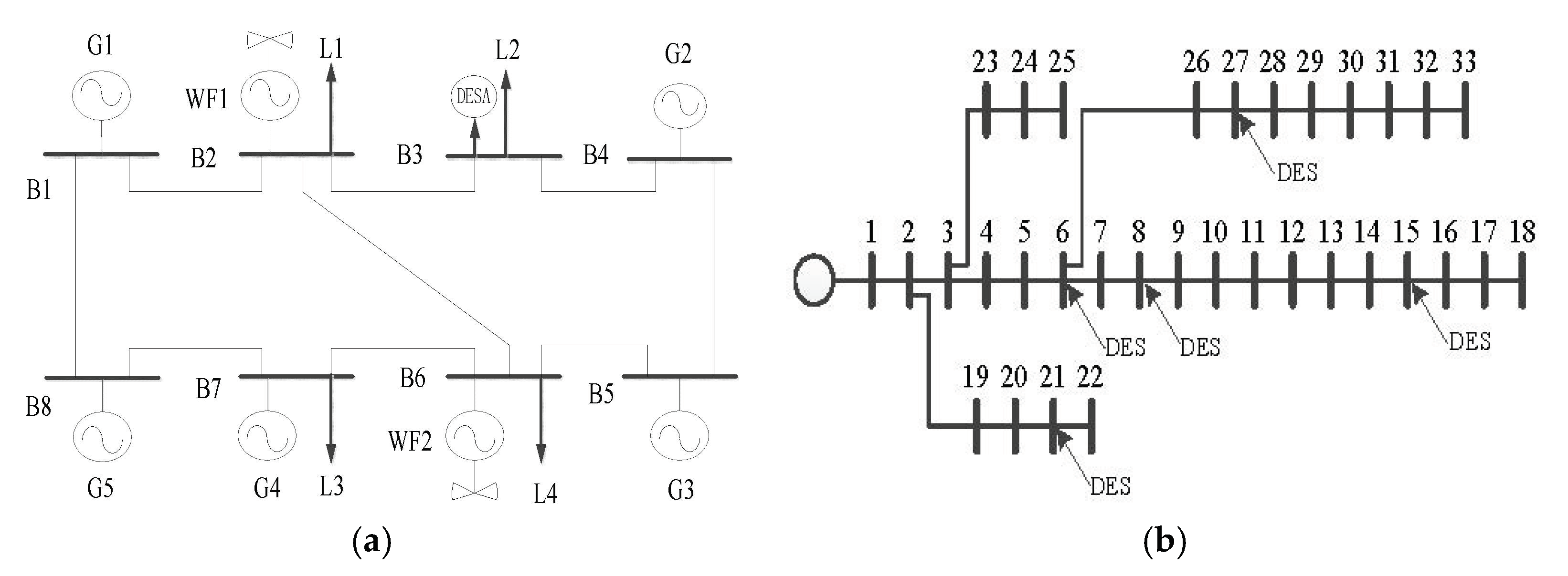
4.1. Test Description

The network topology of the transmission network and distribution network is shown in Figure 2. The eight-bus test system includes five generators, two wind farms, and one DESA. The technical data of generators and the information on transmission lines are given in

Table 1. Technical data of generating units.

Unit	${\overline{\mathit{P}}}_{\mathit{g}}^{}$ (MW)	${\underset{\_}{\mathit{P}}}_{\mathit{g}}^{}$ (MW)	$\mathit{U}{\mathit{t}}_{\mathit{g}},\mathit{D}{\mathit{t}}_{\mathit{g}}$ (h)	$\mathit{R}{\mathit{u}}_{\mathit{g}},\mathit{R}{\mathit{d}}_{\mathit{g}}$ (MW/h)	$\mathit{S}\mathit{d}{\mathit{c}}_{\mathit{g}}$ ($)	$\mathit{S}\mathit{u}{\mathit{c}}_{\mathit{g}}$ ($)	${\overline{\mathit{r}}}_{\mathit{g}}^{\mathit{u}\mathit{p}},{\overline{\mathit{r}}}_{\mathit{g}}^{\mathit{d}\mathit{n}}$ (MW)	${\mathit{C}}_{\mathit{t},\mathit{g}}^{\mathit{G}}$ ($)/MWh	${\mathit{C}}_{\mathit{t},\mathit{g}}^{\mathit{f}}$ ($)/h
G1	100	25	5	30	2550	1200	5	500	32
G2	90	15	4	40	2250	1100	8	400	34
G3	75	10	3	50	2100	1050	10	450	36
G4	72	10	3	55	2000	1000	12	450	36
G5	50	10	2	50	2000	750	10	400	38

and

Table 2. Transmission line data for eight-bus test system.

From Bus	To Bus	X (p.u.)	Transmission Limit (MW)
1	2	0.12	80
1	8	0.38	50
2	3	0.24	60
2	6	0.08	80
3	4	0.4	44
4	5	0.08	80
5	6	0.17	80
6	7	0.16	70
7	8	0.08	80

. These data are adapted from [27] and are adjusted to meet the needs of the test case. The generation capacities of WF1 and WF2 are 55 MW and 45 MW, which are connected to nodes B2 and B6, respectively. The system load curve and forecasted output curve of WPPs are shown in Figure 3. The day-ahead energy market price at node B3 is given in Figure 4. The DESA controls five DES systems, and the rated capacity of DES is 4 MWh. The maximum charging and discharging power of DES is 1 MW. In this test system, a daily (24 h) time horizon is considered. In order to make the test more credible, the daily forecast output scenario set is given by Monte Carlo simulation, shown in Figure 5. These scenarios are reduced through FCMC to form four wind power typical uncertainty scenarios, given in Figure 6. After the scenario reduction, the probabilities of scenarios 1–4 are 0.15, 0.35, 0.33, and 0.17. We assume that the price of providing reserve in DA is $40/MWh and that the price in the balancing market is $55/MWh. The imbalance prices [28] have not been considered in this paper. The hourly maximum reserve capacity of demand is considered to be 20% of forecast wind power output. The CO₂ emission of the unit output is considered to be 0.34 ton/MWh, and the cost of CO₂ pollutant emission is assumed to be $30/ton.

In order to demonstrate the performance of the optimization model, the following three cases are derived and discussed in detail. These cases are tackled by using the above-mentioned formulation, and the solutions and details are presented in the following.

Case 1. The DESA only participates in the DA energy market. The only profit source for the DESA is energy arbitrage over time.

Case 2. The DESA participates in the DA energy and reserve markets, but the balancing market is not considered. The DESA makes a profit from energy trading and reserve revenue.

Case 3. The DESA participates in the DA market and balancing market. The DESA makes a profit from the energy market, reserve revenue, and energy deployed from committed reserve in the balancing market.

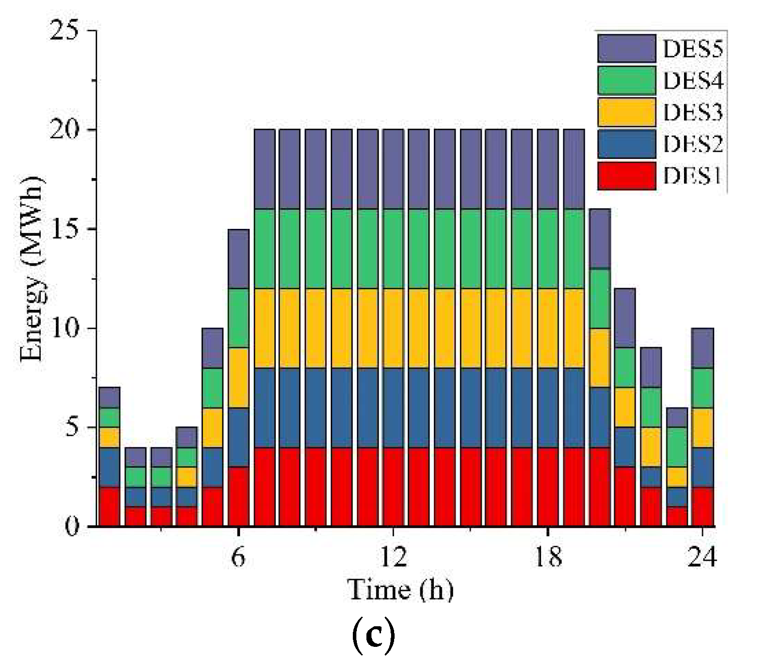
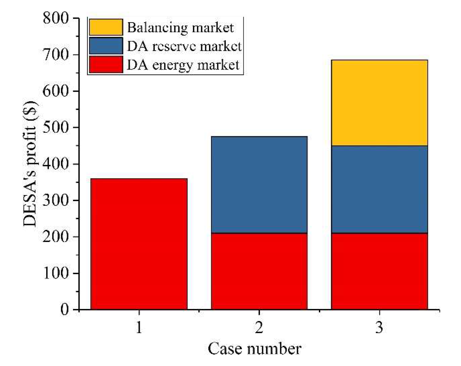
4.2. Simulation Results

This section shows the simulation results of the optimization model in different aspects, such as scheduling power, energy capacity of the DESA and DES, operating cost comparison of units and the DESA, scheduling power, and comparison of reserve capacity of the DESA in different cases.

Figure 7 and Figure 8 show the optimal strategy of units, DESA, and DES in cases 1 and 2 under provided upward reserve. Figure 7a and Figure 8a show the scheduled processes of the generators. The operating cost of G1 is higher than the rest of the generators. Therefore, G1 has the least contribution in the dispatch plan. When the reserve capacity requirement is less than the G1 output gap, G1 will provide reserve capacity in case 1. Due to the DESA participating in the DA reserve market in case 2, the reserve capacity provided by the generators will decrease. Figure 7b shows the optimal strategy of the DESA in case 1. The charge and discharge power of the DESA reach the upper limit. In this way, the DESA could effectively participate in the energy market and reduce the operation cost of the power system. Figure 8b shows the scheduling plan and reserve capacity plan provided by the DESA in case 2. In the case where the DESA provides reserve capacity, its charge and discharge power are under the upper limit, because the DESA needs to set aside some reserve capacity to cope with the error between the scenario wind power output and predicted wind power output. Due to low electricity prices over the time period 04:00–08:00, the DESA controls DES to charge to obtain a high arbitrage profit and tracks the trend of electricity price to maximize profit in the DA energy market. Figure 7c and Figure 8c show the scheduling plan of DES in the corresponding case.

In case 3, we assume that the initial DESA capacity is half of the rated capacity. In this way, the DESA has the greatest potential to provide up-spinning and down-spinning reserve in the balancing market for the power system. Figure 9 shows the energy storage capacity process of the DESA in case 3.

Table 3. Comparison of reserve results for units and DESA in case 3.

Case	Scenario	DESA Up/Downward Reserve Capacity (MWh)	Generation Up/Downward Reserve Capacity (MWh)	DESA Capacity Utilization
3	1	120	61	100%
	2	45	0	75%
	3	43	3	90%
	4	119	65	100%

shows the comparison reserve results of the DESA and units in case 3. The output power of scenarios 1 and 2 is less than the predicted wind power output. The units provide upward reserve. The DESA appears as a discharged state to provide reserve capacity. Therefore, from 0:00 to 6:00, the DESA maintains a discharge state to cope with wind power uncertainties. In scenario 1 from 7:00 to 11:00, the DESA appears as a charged state. It shows that the DESA participated in the energy market during this time. Because the price of electricity in this period is low, the DESA will energy arbitrage and store energy to participate in the reserve market once again. In scenario 2 from 7:00 to 19:00, the DESA appears as a rising fluctuation trend of charged state, because the reserve requirement in scenario 2 is less than scenario 1. While participating in the reserve market, the DESA also tracks electricity prices and arbitrages in the short term in order to maximize revenue. Similarly, the output power of scenarios 3 and 4 is more than the predicted wind power output. The units provide downward reserve. The DESA charges during the initial period to maintain system power balance.

Table 4. Comparison of economic profit for generators in cases 1, 2, and 3.

Case	Scenario	Total Generation Reserve Cost ($)	CO2 Emissions Penalty ($)	Total Generation Cost ($)
1	Provide upward reserve	2840	43,582	1,848,142
2	Provide upward reserve	0	43,582	1,845,302
3	1	1620	42,952	1,835,142
	2	0	41,815	1,829,792
	3	0	41,587	1,829,942
	4	1400	42,882	1,836,692

shows an economic comparison of generators in cases 1, 2, and 3. More operating cost of the power system is gained in case 1 than case 2, because when the DESA trades in the DA reserve market, it fully meets the required reserve capacity of the power system. The generators reduce operating cost due to no reserve capacity. This is why the DESA gains more profit in case 2 compared with case 1 in the DA market, as shown in Figure 10. By comparing scenarios 1–4 in case 3, it can be seen that the higher the forecast wind power output error is, the higher the power system operating cost and CO₂ emission penalty fee are. The DESA participates in the reserve market with no cost, and units trade in the reserve market with operating cost. Therefore, the DESA has higher priority than units in reserve market trading. The DESA’s profit in different cases is compared in Figure 10. There is more profit in case 3 compared with the first two cases due to the availability of more business opportunities, because the DESA deals with wind power output uncertainties in the balancing market. We observe that the DESA maximizes revenue from the DA energy market, reserve market, and balancing market.

5. Conclusions and Future Studies

In this paper, a bilevel model of the DESA participated in the day-ahead energy and reserve capacity markets, and the balancing market have been presented utilizing DESA operating strategy in different markets to deal with the uncertainty of wind power penetration. The resulting problem is an MILP. The optimal DESA strategy has been discussed in the DA energy-only market, the DA energy and reserve, and both energy and reserve markets considering the balancing market. In this framework, the DESA has optimized its operating strategy as a profit-seeking entity in a competitive energy and reserve market. Results show that the DESA has profited more from the reserve market than the energy market for two reasons: (1) it aggregates DES capacity to provide reserve capacity instead of the reserve capacity provided by units, and (2) it gains additional revenue when it trades in the balancing market. After the DESA participated in the electricity market, the units’ expense on the offer cost of reserve capacity and CO₂ emission penalty were reduced.

Future work will focus on improving the cooperation strategy in the optimization model under other flexible loads. More generation technologies and different aggregators will be added to the model. A flexible load aggregator will be built to participate in real-time energy and reserve markets. In addition, the aggregator will play a more important role in trading and bidding in the energy and reserve market as a price-maker.

References

1. ODwyer, C.; Ryan, L.; Flynn, D. Efficient Large-Scale Energy Storage Dispatch: Challenges in Future High Renewable Systems. IEEE Trans. Power Syst. 2017, 32, 3439–3450. [Google Scholar] [CrossRef]
2. Zhang, Y.; Gevorgian, V.; Wang, C.; Lei, X.; Chou, E.; Yang, R. Grid-Level Application of Electrical Energy Storage: Example Use Cases in the United States and China. IEEE Power Energy Mag. 2017, 15, 51–58. [Google Scholar] [CrossRef]
3. Chen, H.; Baker, S.; Benner, S.; Berner, A.; Liu, J. PJM Integrates Energy Storage: Their Technologies and Wholesale Products. IEEE Power Energy Mag. 2017, 15, 59–67. [Google Scholar] [CrossRef]
4. Cao, J.; Du, W.; Wang, H.F. An Improved Corrective Security Constrained OPF With Distributed Energy Storage. IEEE Trans. Power Syst. 2016, 31, 1537–1545. [Google Scholar] [CrossRef]
5. Contreras-Ocana, J.E.; Ortega-Vazquez, M.A.; Zhang, B. Participation of an Energy Storage Aggregator in Electricity Markets. IEEE Trans. Smart Grid 2017, 1. [Google Scholar] [CrossRef]
6. Wang, Y.; Tan, K.T.; Peng, X.Y.; So, P.L. Coordinated Control of Distributed Energy-Storage Systems for Voltage Regulation in Distribution Networks. IEEE Trans. Power Deliv. 2016, 31, 1132–1141. [Google Scholar] [CrossRef]
7. Strbac, G.; Aunedi, M.; Konstantelos, I.; Moreira, R.; Teng, F.; Moreno, R. Opportunities for Energy Storage: Assessing Whole-System Economic Benefits of Energy Storage in Future Electricity Systems. IEEE Power Energy Mag. 2017, 15, 32–41. [Google Scholar] [CrossRef]
8. Singh, A.K.; Parida, S.K. A review on distributed generation allocation and planning in deregulated electricity market. Renew. Sustain. Energy Rev. 2018, 82, 4132–4141. [Google Scholar] [CrossRef]
9. Uddin, M.; Romlie, M.F.; Abdullah, M.F.; Abd Halim, S.; Abu Bakar, A.H.; Chia Kwang, T. A review on peak load shaving strategies. Renew. Sustain. Energy Rev. 2018, 82, 3323–3332. [Google Scholar] [CrossRef]
10. Carpinelli, G.; Celli, G.; Mocci, S.; Mottola, F.; Pilo, F.; Proto, D. Optimal Integration of Distributed Energy Storage Devices in Smart Grids. IEEE Trans. Smart Grid 2013, 4, 985–995. [Google Scholar] [CrossRef]
11. Goebel, C.; Jacobsen, H. Bringing Distributed Energy Storage to Market. IEEE Trans. Power Syst. 2016, 31, 173–186. [Google Scholar] [CrossRef]
12. Awad, A.S.A.; EL-Fouly, T.H.M.; Salama, M.M.A. Optimal ESS Allocation for Benefit Maximization in Distribution Networks. IEEE Trans. Smart Grid 2017, 8, 1668–1678. [Google Scholar] [CrossRef]
13. Jayasekara, N.; Masoum, M.A.S.; Wolfs, P.J. Optimal Operation of Distributed Energy Storage Systems to Improve Distribution Network Load and Generation Hosting Capability. IEEE Trans Sustain Energy 2016, 7, 250–261. [Google Scholar] [CrossRef]
14. Liu, W.; Niu, S.; Xu, H. Optimal Planning of Battery Energy Storage Considering Reliability Benefit and Operation Strategy in Active Distribution System. J. Mod. Power Syst. Cle. 2017, 5, 177–186. [Google Scholar] [CrossRef]
15. Kim, W.; Shin, J.; Kim, J. Operation Strategy of Multi-Energy Storage System for Ancillary Service. IEEE Trans. Power Syst. 2017, 32, 4409–4417. [Google Scholar] [CrossRef]
16. Sarker, M.R.; Dvorkin, Y.; Ortega-Vazquez, M.A. Optimal Participation of an Electric Vehicle Aggregator in Day-Ahead Energy and Reserve Markets. IEEE Trans. Power Syst. 2016, 31, 3506–3515. [Google Scholar] [CrossRef]
17. Hu, J.; Cao, J.; Chen, M.Z.Q.; Yu, J.; Yao, J.; Yang, S. Load Following of Multiple Heterogeneous TCL Aggregators by Centralized Control. IEEE Trans. Power Syst. 2017, 32, 3157–3167. [Google Scholar] [CrossRef]
18. Hao, H.; Sanandaji, B.M.; Poolla, K.; Vincent, T.L. Aggregate Flexibility of Thermostatically Controlled Loads. IEEE Trans. Power Syst. 2015, 30, 189–198. [Google Scholar] [CrossRef]
19. Shayegan-Rad, A.; Badri, A.; Zangeneh, A. Day-ahead Scheduling of Virtual Power Plant in Joint Energy and Regulation Reserve Markets under Uncertainties. Energy 2017, 121, 114–125. [Google Scholar] [CrossRef]
20. Konda, S.R.; Panwar, L.K.; Panigrahi, B.K.; Kumar, R. Optimal Offering of Demand Response Aggregation Company in Price-Based Energy and Reserve Market Participation. IEEE Trans. Ind. Inform. 2018, 14, 578–587. [Google Scholar] [CrossRef]
21. Bahramara, S.; Yazdani-Damavandi, M.; Contreras, J.; Shafie-khah, M.; Catalao, J.P.S. Modeling the Strategic Behavior of a Distribution Company in Wholesale Energy and Reserve Markets. IEEE Trans. Smart Grid 2017, 1. [Google Scholar] [CrossRef]
22. Xu, B.; Wang, Y.; Dvorkin, Y.; Fernandez-Blanco, R.; Silva-Monroy, C.A.; Watson, J. Scalable Planning for Energy Storage in Energy and Reserve Markets. IEEE Trans. Power Syst. 2017, 32, 4515–4527. [Google Scholar] [CrossRef]
23. Nasrolahpour, E.; Kazempour, J.; Zareipour, H.; Rosehart, W.D. A Bilevel Model for Participation of a Storage System in Energy and Reserve Markets. IEEE Trans. Sustain. Energy 2018, 9, 582–598. [Google Scholar] [CrossRef]
24. Akhavan-Hejazi, H.; Mohsenian-Rad, H. Optimal Operation of Independent Storage Systems in Energy and Reserve Markets with High Wind Penetration. IEEE Trans. Smart Grid 2014, 5, 1088–1097. [Google Scholar] [CrossRef]
25. Ruihuan, L.; Yajing, G.; Huaxin, C.; Haifeng, L. Two Step Optimal Dispatch Based on Multiple Scenarios Technique for Active Distribution System with the Uncertainties of Intermittent Distributed Generation and Load Considered. In Proceedings of the IEEE International Conference on Power System Technology, Chengdu, Sichuan, China, 20–22 October 2014; pp. 3303–3308. [Google Scholar]
26. Bouffard, F.; Galiana, F.D. Stochastic Security for Operations Planning with Significant Wind Power Generation. IEEE Trans. Power Syst. 2008, 23, 306–316. [Google Scholar] [CrossRef]
27. Doostizadeh, M.; Aminifar, F.; Ghasemi, H.; Lesani, H. Energy and Reserve Scheduling Under Wind Power Uncertainty: An Adjustable Interval Approach. IEEE Trans. Smart Grid 2016, 7, 2943–2952. [Google Scholar] [CrossRef]
28. Caves-Avila, J.P.; Hakvoort, R.A.; Ramos, A. The Impact of European Balancing Rules on Wind Power Economics and on Short-term Bidding Strategies. Energy Policy 2014, 68, 383–393. [Google Scholar] [CrossRef]
Figure 1. Framework of proposed distributed energy storage aggregator (DESA) in energy and reserve market.
Energies 11 01242 g001
Figure 2. Network topology: (a) eight-bus transmission network; (b) IEEE-33 bus distribution network.
Energies 11 01242 g002
Figure 3. System daily load and wind power forecast output.
Energies 11 01242 g003
Figure 4. Day-ahead market prices at node B3.
Energies 11 01242 g004
Figure 5. Simulated scenarios of wind power output.
Energies 11 01242 g005
Figure 6. Wind power typical uncertainty scenarios.
Energies 11 01242 g006
Figure 7. Hourly schedules of units, DESA, and distributed energy storage (DES) in case 1: (a) optimal power and reserve strategy for units; (b) optimal power strategy for DESA; (c) optimal energy strategy for DES.
Energies 11 01242 g007
Figure 8. Hourly schedules of unit, DESA, and DES in case 2: (a) optimal power and reserve strategy for units; (b) optimal power and reserve strategy for DESA; (c) optimal energy strategy for DES.
Energies 11 01242 g008aEnergies 11 01242 g008b
Figure 9. Comparison of optimal energy strategy for DESA in case 3.
Energies 11 01242 g009
Figure 10. Comparison of economic profit for DESA in cases 1, 2, and 3.
Energies 11 01242 g010