Unit Commitment Towards Decarbonized Network Facing Fixed and Stochastic Resources Applying Water Cycle Optimization

Abstract

This paper presents a trustworthy unit commitment study to schedule both Renewable Energy Resources (RERs) with conventional power plants to potentially decarbonize the electrical network. The study has employed a system with three IEEE thermal (coal-fired) power plants as dispatchable distributed generators, one wind plant, one solar plant as stochastic distributed generators, and Plug-in Electric Vehicles (PEVs) which can work either loads or generators based on their charging schedule. This paper investigates the unit commitment scheduling objective to minimize the Combined Economic Emission Dispatch (CEED). To reduce combined emission costs, integrating more renewable energy resources (RER) and PEVs, there is an essential need to decarbonize the existing system. Decarbonizing the system means reducing the percentage of CO₂ emissions. The uncertain behavior of wind and solar energies causes imbalance penalty costs. PEVs are proposed to overcome the intermittent nature of wind and solar energies. It is important to optimally integrate and schedule stochastic resources including the wind and solar energies, and PEVs charge and discharge processes with dispatched resources; the three IEEE thermal (coal-fired) power plants. The Water Cycle Optimization Algorithm (WCOA) is an efficient and intelligent meta-heuristic technique employed to solve the economically emission dispatch problem for both scheduling dispatchable and stochastic resources. The goal of this study is to obtain the solution for unit commitment to minimize the combined cost function including CO₂ emission costs applying the Water Cycle Optimization Algorithm (WCOA). To validate the WCOA technique, the results are compared with the results obtained from applying the Dynamic Programming (DP) algorithm, which is considered as a conventional numerical technique, and with the Genetic Algorithm (GA) as a meta-heuristic technique.

1. Introduction

The unit commitment study integrating stochastic and disputable resources is a rich topic with different aspects and branches, but all those branches have their scope in the main theme of the work. The guidelines of the introduction are divided into the following points:

• Unit commitment importance and aim of the study;
• The reasons for selecting the objective function governing the unit commitment study, emission cost reduction;
• The advantages and disadvantages of integrating RERs into the study goals;
• The integration of PEVs and their advantages and disadvantages for achieving the quality of the goals
• A state of art in the unit commitment area and the optimization technique applied;
• The contribution and the structure of the paper

Unit commitment is a vital study required to ensure the hourly energy supply requirements. The unit commitment focuses on minimizing the production cost, which mainly depends on the fuel cost value. However, with the increase of fuel cost, the CO₂ emissions will increase. The goal of the study is to decarbonize the CO₂ limit in electrical power system networks, which means reducing the amount of CO₂ emissions. To reduce CO₂ emissions while supplying the required demands, integrating more Renewable Energy Resources (RER) will cause a conflict problem as a result of increasing the amount of CO₂ emissions, which causes the earth temperature to rise. The unit commitment problem is a complicated optimization problem, from the objective function point of view or its constraints [1,2,3,4,5]. The unit commitment problem is defined by scheduling the generation power attained from various power resources. Conventional and intelligent programming techniques are used to solve the unit commitment problem by achieving priority list combination of the generating units, so that the combined emission production cost can be minimized. Many conventional techniques have been applied to solve the unit commitment problem such as the mixed integer optimization [3] and Lagrange method [2,4]. One of the most effective and robust conventional methods is dynamic programming (DP), which is based on the available combinations of resources. This method proves that it is simple and fast and provides autocratic and effective solutions [5]. Due to the large number of resources integrated into the electric grid and the related number of constraints, the need for fast computational technique is urgent. The main purpose of this paper is to provide an optimization framework by scheduling the wind and solar energies and PEVs (load-generator) as stochastic distributed generators and dispatchable distributed generators. This coordination can handle the imbalances of intermittent Renewable Energy Resources (RERs) and encourage PEVs passengers to take part in the demand response while optimal hourly prices are determined.

On the other hand, the international communities seek to prevent temperature rise more than 2 degrees Celsius by generating more energy from domestic resources which can be cost-effective and replaced or renewed without contributing to climatic change or having environmental impacts. Burning fossil fuels such as coal, natural gas and oil, which exhaust ash and gaseous pollutants such as carbon oxides (CO and CO₂) nitrogen oxides (NO_x)) and sulphur dioxide (SO₂) … etc. Electricity production is roughly responsible for half of the greenhouse gas emissions (GHGEs). In fact, it is expected that the fossil-fuel power plants planned to be built, will emit tens of billion tons of carbon dioxide over their expected lifetime, compared with the annual emissions of all fossil-fuel power plants that were operating in the preceding years. Excluding these fossil fuel power plants early is achievable, but the cost comparison for decision-makers who compare fossil fuels with clean energy resources remains a critical issue. Long-term planning will lead to stabilizing climatic changes and achieving zero emissions. Therefore, the goal is decreasing the emissions in the upcoming decades to attain zero net emissions by the end of this century, which can be achieved by applying the unit commitment study. Carbon–neutral electricity can be produced by using renewable resources (windmills, photovoltaic power, concentrated solar power, nuclear power, large dams and small hydropower) and fuel shifting technologies such as electric and plug-in hybrid vehicles in the transportation sector [6].

Renewable energy resources (RERs) in such systems integrate with conventional power plants seeking to achieve potential decarbonization of the electrical system. RERs consist of low-carbon base load generation technologies such as nuclear and fossil fuels with carbon capture and sequestration, along with more modest contributions (25%) from wind (whether on-shore or off-shore), and solar (whether photovoltaic or solar thermal cells) [7]. Solar integration can help in improving and reducing the pollution limits obtained from fossil fuel substations. Encouraging residential customers to use PV solar microgeneration can save 3.5% of energy consumption in addition to reducing the overall cost by 75% lower than the models without PV [8,9,10,11]. Energy storage devices (ESDs) with PV panels can contribute to saving 12% of the energy cost. Hence, this encourages end users with Home Energy Management Systems (HEMSs) to reduce or shift their electricity consumption patterns in response to a price or grid condition signal [12]. By contributing to customers’ payment for the cost of generation as well as for the transmission, distribution and indirect cost of environmental cleanup and health effects, these renewable resources may become attractive when customers face the actual price of electricity production [13].

Because of the uncontrollable behavior of wind speed and solar insolation, the output of wind and solar power generation is unpredictable. Swings in generation of wind and solar energy between oversupply and undersupply will lead to estimations of the hourly contributions from wind and PV as being insufficient to satisfy renewable portfolio standards and overwhelm any conceivable storage strategy. Consequently, wind and solar energies will compensate a part of the load demand. It is necessary to handle the uncertain behavior of these renewable resources which may cause operational risk of power system [14]. Controlling both active and reactive power independently is done to overcome the stochastic nature of wind energy profile by using voltage source inverters (VSIs) based on FACTS devices (STATCOM) + battery energy storage systems (BESS) which will promote the transient and dynamic stability and minimize sub-synchronous oscillations [15]. Battery storage technologies (i.e., pumped hydroelectric storage (PSH)) may have a vital role in solving imbalances due to seasonal swings in the generation output of wind and solar power plants. Furthermore, battery storage will decrease energy costs and support dependence on renewable energy for the off-grid areas (remote locations) not connected to the grid and therefore resort to using expensive imported fuels [14,16].

Exchanging the old generation with the new RERs technologies has proved its efficiency in many cases. For example, in Tasmania, the diesel consumption of King Island has fallen to 50% after exchanging renewable energy and battery storage for the conventional power plants [17]. Another example is found in an existing network of Masirah Island, where the hybrid energy system is composed of fuel-fired, photovoltaic and wind generator units is considered the most economically feasible combination. Despite the high capital costs of this combination, it provides the cheapest operating cost, energy cost and hence the lowest net running cost. This combination of units also enhances the voltage profile of the system [18]. In 2013, as leading global steps in renewable energy, the German government encouraged utility and smaller-scale battery storage by introducing many incentives for households, companies, local authorities and community organizations. Households and businesses could access grants for 30% of the upfront installation costs to install new solar PV and storage systems [14,16]. The energy storage system (ESS) can provide an alternative by satisfying peak demand to achieve load levelling and peak reduction of up to 8% by using GA in the UK distribution network with a peak capacity violation [19].

Plug-in electric vehicles are expected to become widely common in the upcoming decades. 2010 witnessed release of the first plug-in hybrid Chevy Volt made by General Motors and the all-electric Leaf was released by Nissan. In the first half of 2017, the sales of new vehicles were 50 percent higher than sales in 2016 and it is predicted that new global PEV sales will exceed this percentage compared with traditional fuel vehicle sales by 2050 [14,16]. Encouraging passengers to use PEV to shift peak load will help in supplying load in uncertainty situations [20]. Reasons for the optimistic forestation of plug-in electric vehicles include:

• They are quiet due to reducing the tailpipe emissions and air pollutants produced by gasoline or diesel-powered engines which harm the heart and lung health for the people living near roads;
• They require less maintenance;
• Recharging is cheaper than refueling with petrol which is a depleted energy resource, leading to less reliance on fossil fuels if powered by renewable energy;
• The vehicle battery can also be used for household electricity storage [21,22].

Plug-in electric vehicles (PEVs) can be considered as a battery storage based on the concept of battery energy storage systems in which vehicles operate with an electric motor that can be powered by an external electrical source. From a grid perspective, two basic types of EVs are typically indicated to BEVs as the battery is considered a primary source of power in EVs, or plug-in hybrid electric vehicles (PHEVs) are combined with a secondary drive option. Some models feature a gasoline-powered engine such as the internal combustion engine (ICE). The battery capacity ranges from less than 10 kWh to over 80 kWh. However, the battery charging and discharging process in PEVs may cause sharp, unexpected spikes in electric power consumption and lead to potential grid issues [23]. PEVs support grid operation by providing distributed energy storage in the form of vehicle to grid (V2G). After optimally determining the appropriate size for renewable resources and storage devices [24,25], the optimal scheduling takes place. By the optimal intelligent scheduling of PEVs, V2G potentially provides grid generation to reduce the intermittency and uncertainty of renewable resources such as wind and solar power [26].

Charging of PEVs can be scheduled at night as well as during weekends, when electricity prices are comparatively low and when vehicles are not used. However, some PEVs charging will be needed during the daylight and even during peak demand or rush hour intervals when the grid already provides the maximum electric power capacity [27]. There are two methods of the charging strategy of the scheduling PEVs, namely, the reactive strategy and the proactive strategy. The reactive strategy: As soon as the PEVs have been plugged-in, some unnecessary loads like heaters and dryers are postponed for decreasing the base load. Non-critical but high consuming loads can be turned off by the center controller until the battery of PEVs is being fully charged. However, the domestic loads cannot be easily controlled. The proactive strategy estimates the averages charging scenario and the future capacity to avoid overloading with the day-ahead load profile. During fast charging process, the proactive method may cause a sudden spike, but may take a shorter charging interval. The reactive method can handle the deviation risk, but charging process occur in more time [28].

Due to the complexity of the problem, there is a crucial need for a powerful optimization technique to find the optimal solution which satisfies the objective and the constraints [29,30,31,32,33]. The water cycle optimization algorithm is applied to solve the economical emission dispatch unit commitment problem. The algorithm is considered a new meta-heuristic technique where the obtained results will be compared with another heuristic technique such as the genetic algorithm (GA) and traditional technique as dynamic programming (DP). The contribution of this paper mainly appears in scheduling the PEVs as load-generators, the construction of the optimization function including the emission cost not as a penalty [2], but as a cost that should be paid, and applying the WCOA in a new field to validate its performance with respect to other conventional and meta-heuristic techniques.

The paper is divided into seven sections. Section 2 presents an overview of the unit commitment formulation and constraints and outlines the steps and procedures of the Dynamic Programming technique. Section 3 delivers the main rules and concepts about the Water Cycle Algorithm. Section 4 represents the data of the system under study. Simulation results are illustrated in Section 5. Section 6 summarizes the discussion main points, while Section 7 presents the paper’s conclusions. Also, a summary of all variables and acronomies is displayed.

2. Unit Commitment Formulation

Unit commitment formulation in this study can be considered as a multi-objective, single function representation optimization problem which aims to minimize both the operating cost and the emission cost. Not only the renewable energy resources (RER) such as wind and solar energies will be added to the electric industry to decrease the emission, but the PEV as well. The PEV will be used to reduce both the cost and the emission in the electricity and transportation sectors. The operating cost of the thermal units includes the fuel cost depending on the amount of fuel consumption by the thermal generating units and the start-up cost depending on the temperature of the boilers:

$$\mathrm{Fuel}\mathrm{thermal}\cos \mathrm{t}={\displaystyle {\displaystyle \sum }_{\mathrm{i}=1}^{{\mathrm{N}}_{\mathrm{G}}}}{A}_i+B_i{\mathrm{P}}_{\mathrm{G}}i+C_i{\mathrm{P}}_{\mathrm{G}}^{2}i$$

(1)

where; ${\mathrm{P}}_{\mathrm{G}}i$ is the output power of each thermal unit “i” at each hour. A, B, C are the coefficients of a quadratic fuel cost function of each thermal generating unit. N_G is the number of conventional thermal units.

A linear model is used to evaluate the fuel cost of wind and solar energy:

$$\mathrm{Fuel}\cos \mathrm{t}\left(\mathrm{wind}/\mathrm{solar}\right)=\left(\mathrm{wind}/\mathrm{solar}\right)\mathrm{price}\times {\mathrm{P}}_{\mathrm{wind}/\mathrm{solar}}$$

(2)

where; ${\mathrm{P}}_{\mathrm{wind}/\mathrm{solar}}$ is the output power from wind or solar plants at each hour. $\left(\mathrm{wind}/\mathrm{solar}\right)\mathrm{price}$ is the coefficient of a linearized fuel cost function of wind or solar plants at each hour:

$$\mathrm{Emission}\cos \mathrm{t}={\displaystyle {\displaystyle \sum }_{i=1}^{{\mathrm{N}}_{\mathrm{G}}}}\mathsf{\alpha }\times {10}^3\times {\mathrm{P}}_{\mathrm{G}}i\times \mathsf{\beta }$$

(3)

where α is CO₂ emission factor that represents the ratio between the quantity of gas emitted (in ton) per unit of energy production (in kWh). β is the emission penalty factor in voluntary markets for planning purposes which is around 10–15 $/ton CO₂ by the end of 2017 [27]. β is defined to be the average of carbon prices, according to the World Bank’s annual Carbon Pricing Watch Report 2017.

The CO₂ emission factor (α) is shown in

Table 1. CO₂ emission factor “α” for different energy resources [34].

Energy Resource	CO2 Emission Factor (Ton/kWh)
Wind	21.0 × 10−6
Hydro	15.0 × 10−6
Solar	6.00 × 10−6
Natural Gas	5.99 × 10−4
Fuel oil	8.93 × 10−4
Coal	9.55 × 10−4

, together with the emission factor of energy resources for both burnt fossil fuels (natural gas, fuel oil and coal) and renewable energy resources (wind, hydropower and solar photovoltaic).

PEVs Operating Constraints

Conventional thermal (coal-fired) units, RERs and PEVs which smartly operate as loads, energy storages or small portable power plants (energy sources) should meet and supply the whole load demand (hour) and the system losses which are described as follows:

• If PEVs are operated as an energy resource or a small power plant:

  $$\begin{array}{ll}{\displaystyle {\displaystyle \sum }_{i=1}^{\mathrm{N}}}{\mathrm{P}}_{\mathrm{G}}i\left(\mathrm{hour}\right)& +{\mathrm{P}}_{\mathrm{wind}}\left(\mathrm{hour}\right)+{\mathrm{P}}_{\mathrm{solar}}\left(\mathrm{hour}\right)+{\displaystyle {\displaystyle \sum }_{j=1}^{{\mathrm{N}}_{\mathrm{V}2\mathrm{G}}\left(\mathrm{hour}\right)}}\mathsf{\eta }{\mathrm{P}}_{\mathrm{P}\mathrm{E}\mathrm{V}\mathrm{j}}\left(\mathrm{hour}\right)\left[{\Psi }_{\mathrm{Pres}}\left(\mathrm{hour}\right)-{\Psi }_{\mathrm{dep}}\left(\mathrm{hour}\right)\right]\\ & =\mathrm{Demand}\left(\mathrm{hour}\right)+\mathrm{Reserve}\left(\mathrm{hour}\right)\end{array}$$

  (4)
• If PEVs are added to the demand as loads:

  $$\begin{array}{ll}{\displaystyle {\displaystyle \sum }_{i=1}^{\mathrm{N}}}{\mathrm{P}}_{\mathrm{G}}i\left(\mathrm{hour}\right)& +{\mathrm{P}}_{\mathrm{wind}}\left(\mathrm{hour}\right)+{\mathrm{P}}_{\mathrm{solar}}\left(\mathrm{hour}\right)=\mathrm{Demand}\left(\mathrm{hour}\right)+\mathrm{Reserve}\left(\mathrm{hour}\right)\\ & +{\displaystyle {\displaystyle \sum }_{j=1}^{{\mathrm{N}}_{\mathrm{V}2\mathrm{G}}\left(\mathrm{hour}\right)}}\mathsf{\eta }{\mathrm{P}}_{\mathrm{P}\mathrm{E}\mathrm{V}\mathrm{j}}\left(\mathrm{hour}\right)\left[{\Psi }_{\mathrm{Pres}}\left(\mathrm{hour}\right)-{\Psi }_{\mathrm{dep}}\left(\mathrm{hour}\right)\right]\end{array}$$

  (5)

  where; ${\mathrm{P}}_{\mathrm{G}}i$ is the output power of each thermal unit “i” at each hour. ${\mathrm{P}}_{\mathrm{P}\mathrm{E}\mathrm{V}\mathrm{j}}$ is the power of each vehicle j, $\mathsf{\eta }$ is plug in vehicle system efficiency. ${\mathrm{N}}_{\mathrm{V}2\mathrm{G}}$ is number of vehicles that are connected to the network at this hour. N is number of units that are on in the unit commitment problem at each hour. ${\Psi }_{\mathrm{Pres}}$ & ${\Psi }_{\mathrm{dep}}$ are the present and the departure state of charge (SOC) respectively.

Some Other Constraints

The generating power limit for each generating unit should be within the minimum and maximum limits:

P_Gi_min ≤ P_Gi ≤ P_Gi_max

(6)

where; P_Gi_min & P_Gi_max are the minimum and maximum output limits of the i-th thermal unit respectively, considering ramp up/down rate, minimum up/down time and the spinning reserve of the system at each hour, which will be required to preserve the reliability and the adequacy of the system. Only the recorded vehicles will contribute to the smart operation according to predetermined scheduling intervals:

$${\displaystyle {\displaystyle \sum }_{\mathrm{hour}=1}^{24}}{\mathrm{N}}_{\mathrm{V}2\mathrm{G}}\left(\mathrm{hour}\right)={\mathrm{N}}_{\mathrm{V}2\mathrm{G}\max }$$

(7)

where; ${\mathrm{N}}_{\mathrm{V}2\mathrm{G}}$ is the number of vehicles connected to the network at this hour. ${\mathrm{N}}_{\mathrm{V}2\mathrm{G}\max }$ is the total number of vehicles in the network.

To avoid loss of battery life:

$${\Psi }_{\min }\left(\mathrm{hour}\right){\mathrm{P}}_{\mathrm{P}\mathrm{E}\mathrm{V}\mathrm{j}}\le {\mathrm{P}}_{\mathrm{P}\mathrm{E}\mathrm{V}\mathrm{j}}\left(\mathrm{hour}\right)\le {\Psi }_{\max }\left(\mathrm{hour}\right){\mathrm{P}}_{\mathrm{P}\mathrm{E}\mathrm{V}\mathrm{j}}$$

(8)

where; ${\Psi }_{\min }$ is the depletion of storage energy at minimum level. ${\Psi }_{\max }$ is the charging up to maximum level.

The multi-objective single-representation objective function for Cost Emission Economical Dispatch (CEED) optimization that is required to be minimized in the smart grid is expressed as follows:

$$\begin{array}{c}\mathrm{CEED}=\mathrm{Minimize}\mathrm{total}\cos \mathrm{t}=\min \left\{\mathrm{fuel}\cos \mathrm{t},\mathrm{start}-\mathrm{up}\cos \mathrm{t},\mathrm{emission}\right\}\\ ={\displaystyle {\displaystyle \sum }_{i=1}^{\mathrm{N}}}{\displaystyle {\displaystyle \sum }_{hour=1}^{24}}\{\mathrm{Fuel}\mathrm{thermal}\cos \mathrm{t}({\mathrm{P}}_{\mathrm{G}}i\left(\mathrm{hour}\right))+\mathrm{Fuel}\cos \mathrm{t}\left(\mathrm{wind}/\mathrm{solar}\right)\left(\mathrm{hour}\right)+\\ \mathrm{start}-\mathrm{up}\cos \mathrm{ti}\left(\mathrm{hour}\right)\times \left(1-\mathrm{U}i \left(\mathrm{hour}-1\right)\right)+\mathrm{Emission}\cos \mathrm{t}\left(\mathrm{P}i\left(\mathrm{hour}\right)\right)\}\times \mathrm{U}i\left(\mathrm{hour}\right)\end{array}$$

(9)

where, $\mathrm{U}i\left(\mathrm{hour}\right)$ is on/off state of each unit i.

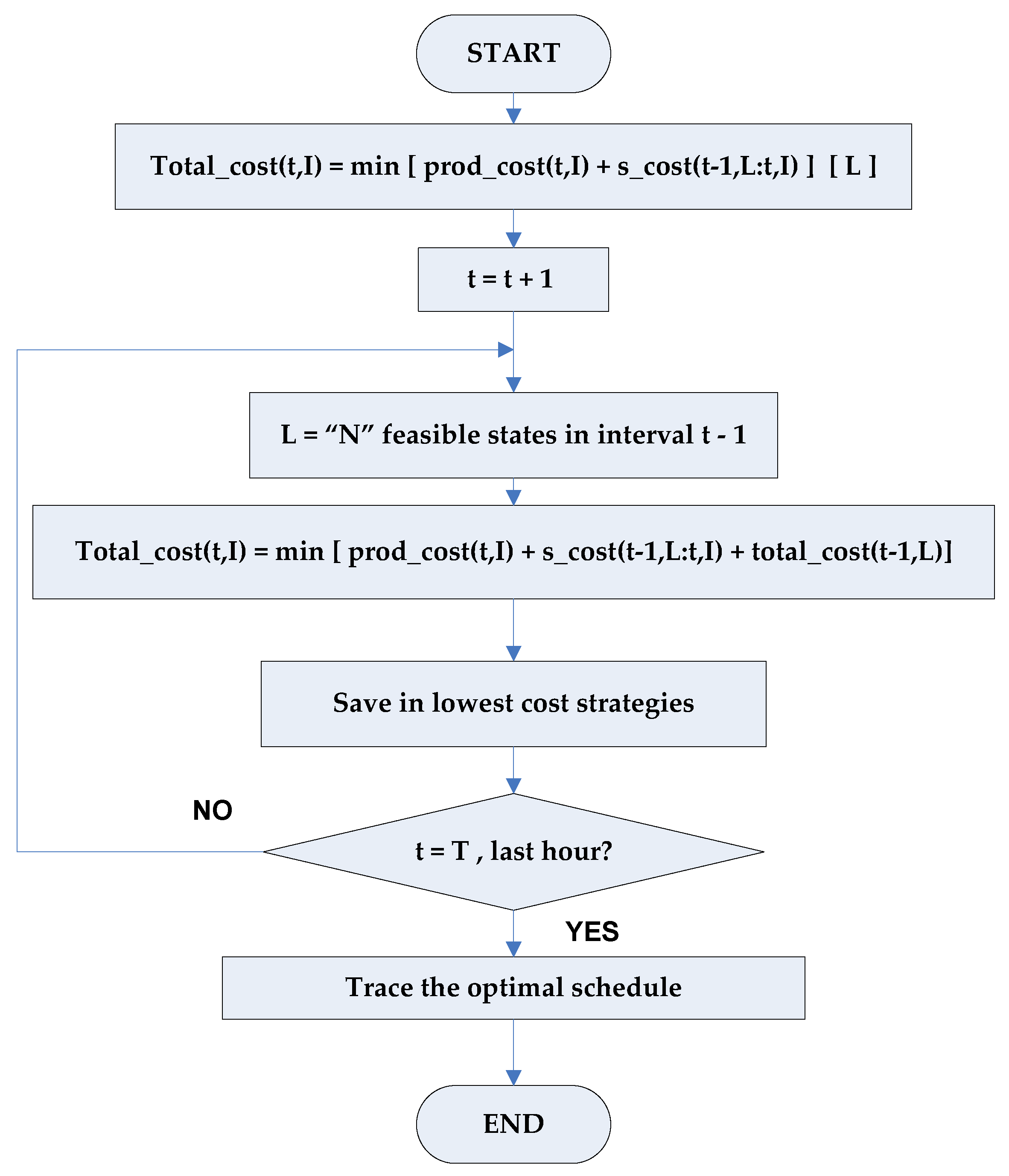
2.1. Unit Commitment Solution Using Dynamic Programming Technique

In 1957, Bellman interpreted the theory of dynamic programming (DP). Combination of the generating units is considered as the states which need to be determined. Searching for the optimum solution is achievable for each time interval (hour) in a forward or backward direction.

In forward direction of dynamic programming, the optimistic economic combination of the minimum accumulated cost starts at the last stage and ends at the initial stage. The stages form the intervals of the study problem considered as T = 24 h. The combination of each generating unit forwards one hour, then the arrangement is scheduled and stored for each hour. Eventually, at the final hour, the best path of the most economical schedule of the generating power for each unit is attained by backward pedaling. The main advantage of this method is that the dimensionality of the problem can be significantly ignored, so that dynamic programming can get the best path of the minimum cost for running N_G units [35,36].

2.2. Step by Step Tracking for Dynamic Programming

The dynamic programming approach is based on the probabilities of generators to supply the load at a certain hour, satisfying the constraints to achieve the objective function which minimizes the combined emission costs. The dynamic programming algorithm for unit commitment problem, in its elemental form, tackles every probable state in every interval. The algorithm is based on the posterior repeating equation:

$$\mathrm{Total}\_\cos \mathrm{t}\left(\mathrm{t},\mathrm{I}\right)=\min \left[\mathrm{prod}\_\cos \mathrm{t}\left(\mathrm{t},\mathrm{I}\right)+\mathrm{s}\_\cos \mathrm{t}\left(\mathrm{t}-1,\mathrm{L}:\mathrm{t},\mathrm{I}\right)+\mathrm{total}\_\cos \mathrm{t}\left(\mathrm{t}-1,\mathrm{L}\right)\right]$$

(10)

where total_cost(t,I) is the least total cost required to arrive at state (t,I); prod_cost(t,I) is the production cost at state (t,I); and s_cost(t − 1,L: t,I) is the transition cost from state (t − 1,L) to state (t,I).

Strategy in forward dynamic programming is defined as the transition or path from one state at a given hour to a state at the next hour. The state (t, 1) is the I-th combination in hour t, where N is the number of strategies to save at each step and X is the number of states to search each period. The maximum value of X or N is 2^N − 1. The presumption for the step by step procedure and the flowchart of the dynamic programming method are expressed in Figure 1 and explained as follows:

(a)

A state is composed of an arrangement of generating units with only accurate units in service, operating at a time while the remaining units are off-line.

(b)

The start-up cost of each unit is fixed and independent of the time, whether or not the generating unit is in off state.

(c)

No cost is involved for the shutdown of the unit.

(d)

At each interval, the order of priority is firm and a small amount of power should be in operation.

By increasing number of resources in the network, the number of permutations and combinations will become hectic. So the crucial need to find the optimal solution in an intelligent way is important to save time and complexity. The water cycle algorithm, genetic algorithm compared to the quad programming is exposed showing the power and the efficiency of the applied algorithm.

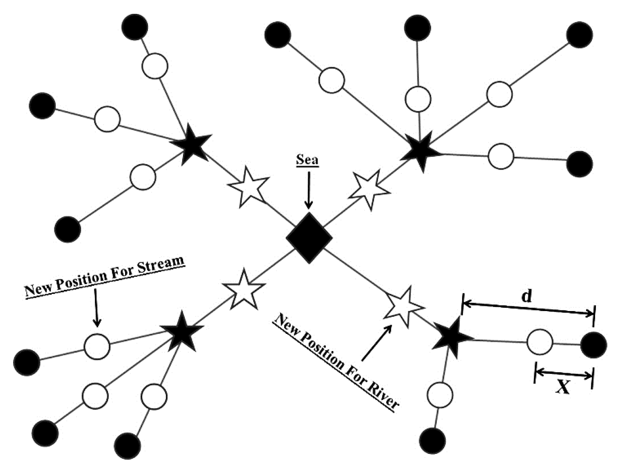
3. The Water Cycle Optimization Algorithm (WCOA)

In 2013, the water cycle algorithm (WCA) is considered as a meta-heuristic technique. The new technique is used to obtain the optimal solutions for problems. The main concept of constructing the water cycle algorithm is inspired by the natural phenomena of the water cycle. The flow of the rivers and streams into the sea occurs as in real life as illustrated in Figure 2. Water is formed from rain, other streams or high up in the mountains, when snow and glaciers melt. Water travels downhill and forms a river or a stream. Rivers and streams flow downhill on their journey towards the sea.

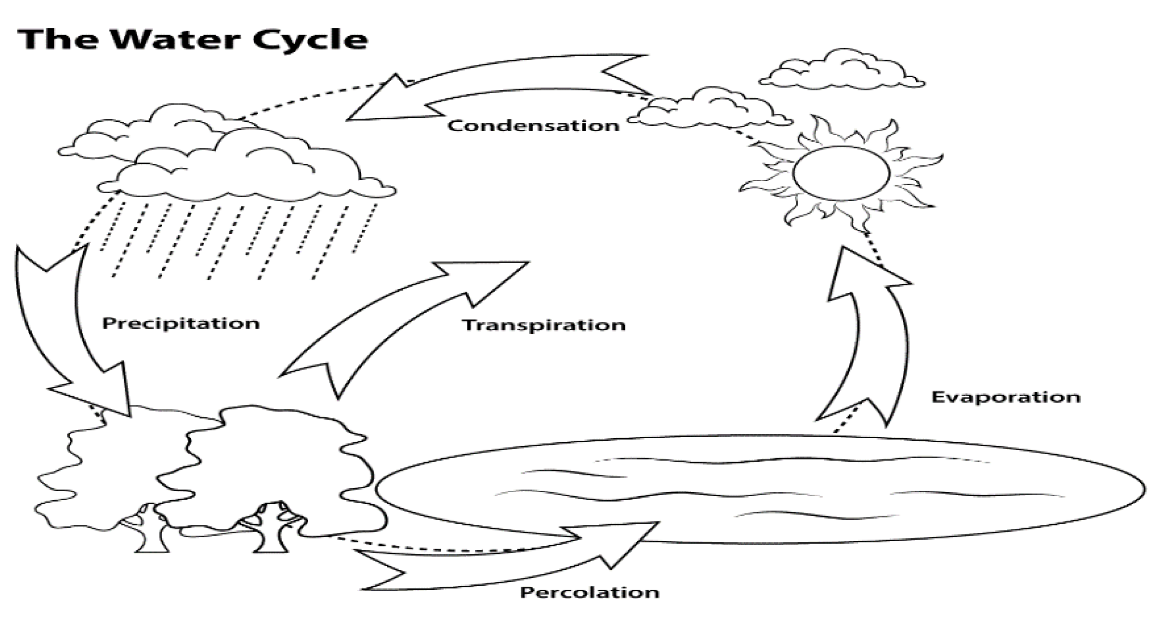
3.1. Hydrologic Cycle

The hydrologic cycle consists of:

• Evaporation process: Because of high temperatures, water in lakes and rivers evaporate.
• Transpiration process: During photosynthesis, plants transpire and give off water.
• Condensation process: The water evaporated from rivers and the water transpired by trees generate clouds when such water is condensed into the colder atmosphere.
• Precipitation process: The water is released back to the earth in the form of rain
• Percolation process: When rain falls and glaciers melt, the water is reserved beneath the ground. The groundwater, aquifer, flows downward in the same way water flows on the ground surface completing the hydrologic cycle [37].

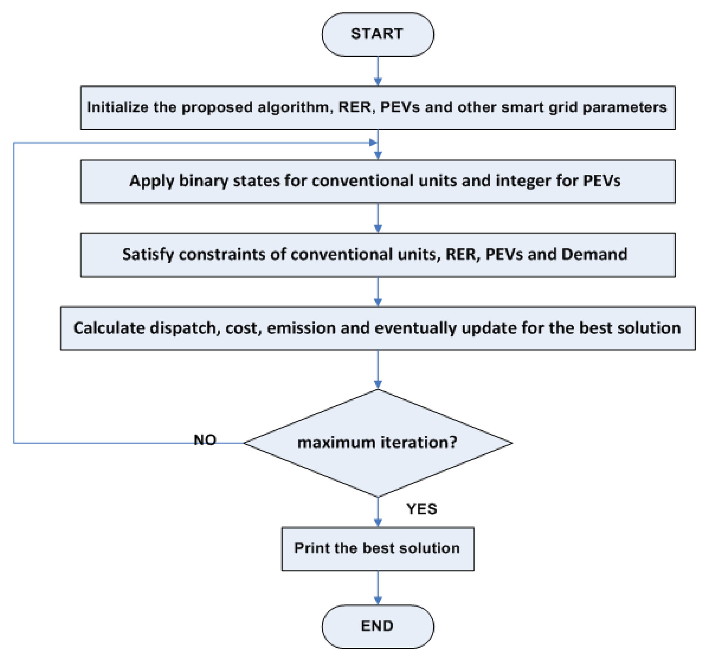
3.2. The Proposed WCOA

Similar to other meta-heuristic algorithms, rain or precipitation forms raindrops which are considered as the initial population in the proposed algorithm. When the best raindrop is found, the best individual (raindrop) is selected as a sea. Many good raindrops are selected as a river and the rest are considered as streams which flow into the rivers and the seas. Using the population based meta-heuristic techniques “Raindrop” is a single solution in an array of 1 × N_var, where N_var is a dimensional optimization problem or number of the design variable [38,39]:

$$\mathrm{Raindrop}=\left[{\mathrm{X}}_1,{\mathrm{X}}_2,{\mathrm{X}}_3\dots {\mathrm{X}}_{\mathrm{N}}\right]$$

(11)

A population of raindrops is generated as a matrix of raindrops of size N_pop × N_var, where N_pop is the number of population as per the following Equation (12):

$$\mathrm{Population}\mathrm{of}\mathrm{raindrops}=\left[\begin{array}{c}{\mathrm{Raindrop}}_1\\ {\mathrm{Raindrop}}_2\\ \begin{array}{c}⋮\\ ⋮\\ {\mathrm{Raindrop}}_{{\mathrm{N}}_{\mathrm{pop}}}\end{array}\end{array}\right]=\left[\begin{array}{ccc}{\mathrm{X}}_1^1& {\mathrm{X}}_2^1& \begin{array}{cc}{\mathrm{X}}_3^1& \begin{array}{cc}\dots & {\mathrm{X}}_{{\mathrm{N}}_{\mathrm{var}}}^1\end{array}\end{array}\\ {\mathrm{X}}_1^2& {\mathrm{X}}_2^2& \begin{array}{cc}{\mathrm{X}}_3^2& \begin{array}{cc}\dots & {\mathrm{X}}_{{\mathrm{N}}_{\mathrm{var}}}^2\end{array}\end{array}\\ \begin{array}{c}⋮\\ {\mathrm{X}}_1^{{\mathrm{N}}_{\mathrm{pop}}}\end{array}& \begin{array}{c}⋮\\ {\mathrm{X}}_2^{{\mathrm{N}}_{\mathrm{pop}}}\end{array}& \begin{array}{cc}\begin{array}{c}⋮\\ {\mathrm{X}}_3^{{\mathrm{N}}_{\mathrm{pop}}}\end{array}& \begin{array}{cc}\begin{array}{c}⋮\\ \dots \end{array}& \begin{array}{c}⋮\\ {\mathrm{X}}_{{\mathrm{N}}_{\mathrm{var}}}^{{\mathrm{N}}_{\mathrm{pop}}}\end{array}\end{array}\end{array}\end{array}\right]$$

(12)

where (X₁, X₂, X₃,…, X_Nar) are the decision variable values which can be defined as floating point number (real values) for continuous and discrete problems. The cost function of raindrops is represented in the following Equation (13):

$$C_i={\mathrm{Cos}\mathrm{t}}_i=\mathrm{f}\left({\mathrm{X}}_1^i,{\mathrm{X}}_2^i,{\mathrm{X}}_3^i,\dots ,{\mathrm{X}}_N^i\right),i=1,2,3,\dots ,{\mathrm{N}}_{\mathrm{pop}}.$$

(13)

Seas and rivers are chosen as minimum values (the best individuals). N_sr is defined as the summation of the number of rivers, which is considered as a user parameter and a single sea. The other raindrops (population) flow either to the rivers or directly to the sea as per the following equations:

$${\mathrm{N}}_{\mathrm{sr}}=\mathrm{Number}\mathrm{of}\mathrm{Rivers}+1,\mathrm{where}1\mathrm{is}\mathrm{for}\mathrm{one}\mathrm{sea}$$

(14)

$${\mathrm{N}}_{\mathrm{Raindrops}}={\mathrm{N}}_{\mathrm{pop}}-{\mathrm{N}}_{\mathrm{sr}}$$

(15)

The intensity of the flow determines how to assign raindrops to the rivers and the sea as follows:

$${\mathrm{NS}}_{\mathrm{n}}=\mathrm{round}\{\left|\frac{Cos{t}_n}{{\sum }_{i=1}^{{\mathrm{N}}_{\mathrm{sr}}}Cos{t}_i}\right|\times {\mathrm{N}}_{\mathrm{Raindrops}}\},\mathrm{n}=1,2,\dots ,{\mathrm{N}}_{\mathrm{sr}}.$$

(16)

where NS_n is defined as the number of streams, which travels towards certain rivers or the sea. Figure 3 describes the WCA optimization process in which X is the distance between the stream and the river, can be randomly chosen as follows:

$$\mathrm{X}\in \left(0, \mathrm{C}\le \mathrm{d}\right),1<\mathrm{C}<2$$

(17)

where C is between 1 and 2.; and d is defined as the current distance between stream and river. The value of X in Equation (17) is set according to a randomly distributed number whether (uniformly or in an appropriate distribution) between 0 and (C × d). Enabling C > 1, streams are permitted to flow in various directions towards rivers. This concept can explain rivers flowing into the sea. Therefore, from the point of the exploitation phase in the WCOA, the new position for streams and rivers can be obtained as follows:

$${\mathrm{X}}_{\mathrm{stream}}^{i+1}={\mathrm{X}}_{\mathrm{stream}}^i+\mathrm{rand}\times \mathrm{C}\times \left({\mathrm{X}}_{\mathrm{River}}^i-{\mathrm{X}}_{\mathrm{stream}}^i\right)$$

(18)

$${\mathrm{X}}_{\mathrm{River}}^{i+1}={\mathrm{X}}_{\mathrm{River}}^i+\mathrm{rand}\times \mathrm{C}\times \left({\mathrm{X}}_{\mathrm{Sea}}^i-{\mathrm{X}}_{\mathrm{River}}^i\right)$$

(19)

where rand is a randomly distributed number in a uniform way between 0 and 1. If the solution obtained by a stream is better than its linking river, the positions of river and stream are swapped (i.e., stream becomes river and river becomes stream). The same exchange can occur for rivers and the sea as shown in Figure 4. In the evaporating process, the assumption of evaporating water as streams or rivers is to bypass enclosing in local optima. Therefore, the following Pseudo code is to determine whether or not river flows into the sea.

If |X iSea − X iRiver| < d_max; i = 1, 2, 3,…, (N_sr, the evaporation and raining process will be ended.

Where d_max is considered as a small number and its value is near to zero. Therefore, the distance between a river and sea should be less than d_max. It indicates that the river is linked to the sea, the evaporation process occurs; and the precipitation process (raining) is applied after some adequate evaporation. To get the optimum solution, d_max will control the search intensity close to the sea.

$${\mathrm{d}}_{\max }^{i+1}={\mathrm{d}}_{\max }^i-\frac{{\mathrm{d}}_{i\max }}{\max -\mathrm{iteration}}$$

(20)

where if ${\mathrm{d}}_{\max }^i$ is large, the search is decreased while a small value will be helpful to search close to the sea. In the precipitation process, the new position of the new streams formed by the new raindrops is expressed as follows:

$${\mathrm{X}}_{\mathrm{Stream}}^{\mathrm{new}}=\mathrm{LB}+\mathrm{rand}\times \left(\mathrm{UB}-\mathrm{LB}\right)$$

(21)

where LB and UB are represented as lower and upper boundaries of the designed problem in the proposed algorithm and from the point of the exploration phase. Equation (22) is applied only for the constrained problems to enhance the streams which directly travel toward the sea:

$${\mathrm{X}}_{\mathrm{Stream}}^{\mathrm{new}}={\mathrm{X}}_{\mathrm{Sea}}+\sqrt{\mathrm{\mu }}\times \mathrm{randn}\left(1,{\mathrm{N}}_{\mathrm{var}}\right)$$

(22)

where µ is considered as a coefficient to get the range of searching area close to the sea and the value should be smaller to improve the search in a smaller area. From the mathematical point of view $\sqrt{\mathrm{\mu }}$ is described as the standard deviation and µ is the variance. The best value of µ is 0.1 to get the optimum solution (sea) [32]. For terminating the algorithm, the best solution is obtained at the maximum number of iteration, “ε” (CPU time) is a small and non-negative number which is the allowable tolerance between two successive solutions.

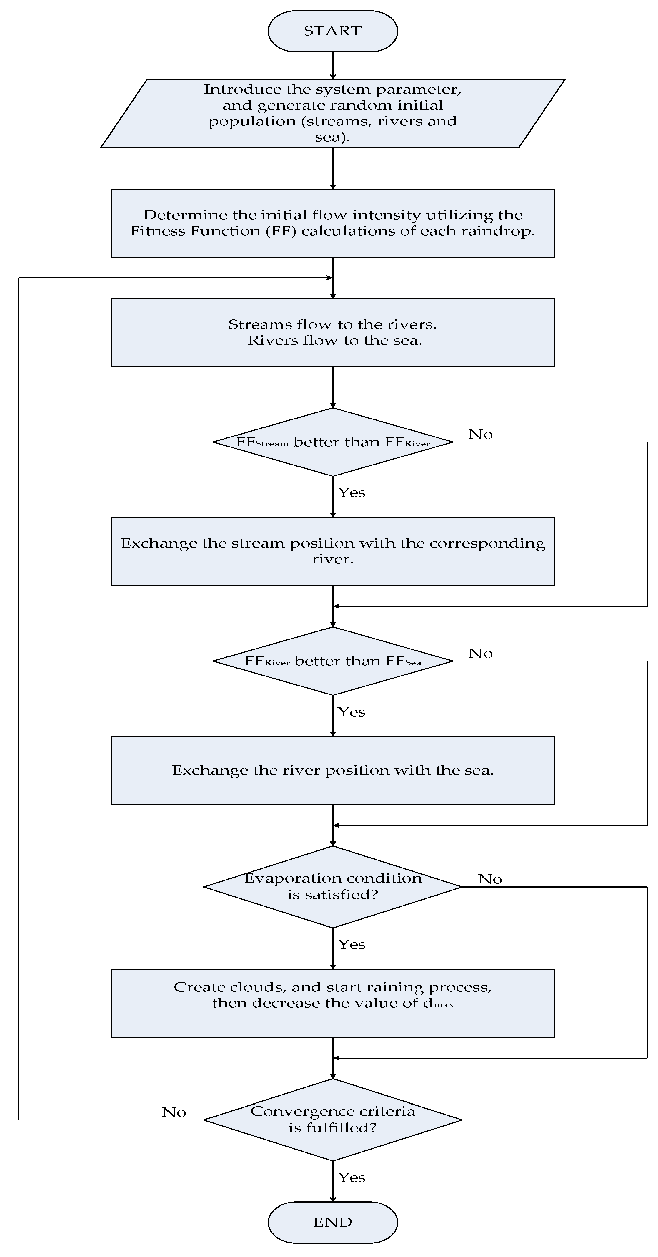
3.3. Step by Step Tracking and the Water Cycle Optimization Algorithm Flowchart

• Step 1: initialize the parameters of WCOA: N_sr, d_max, N_pop, max_iteration.
• Step 2: create a random generation of initial population and generate the initial raindrops, rivers and sea by using Equations (12), (14) and (15).
• Step 3: determine the cost of each stream (raindrops) by using Equation (13).
• Step 4: evaluate the intensity of flow for rivers and sea by using Equation (16).
• Step 5: evaluate the flow of streams into the rivers by using Equation (18).
• Step 6: evaluate the flow of rivers into the sea which has the most downhill place by using Equation (19).
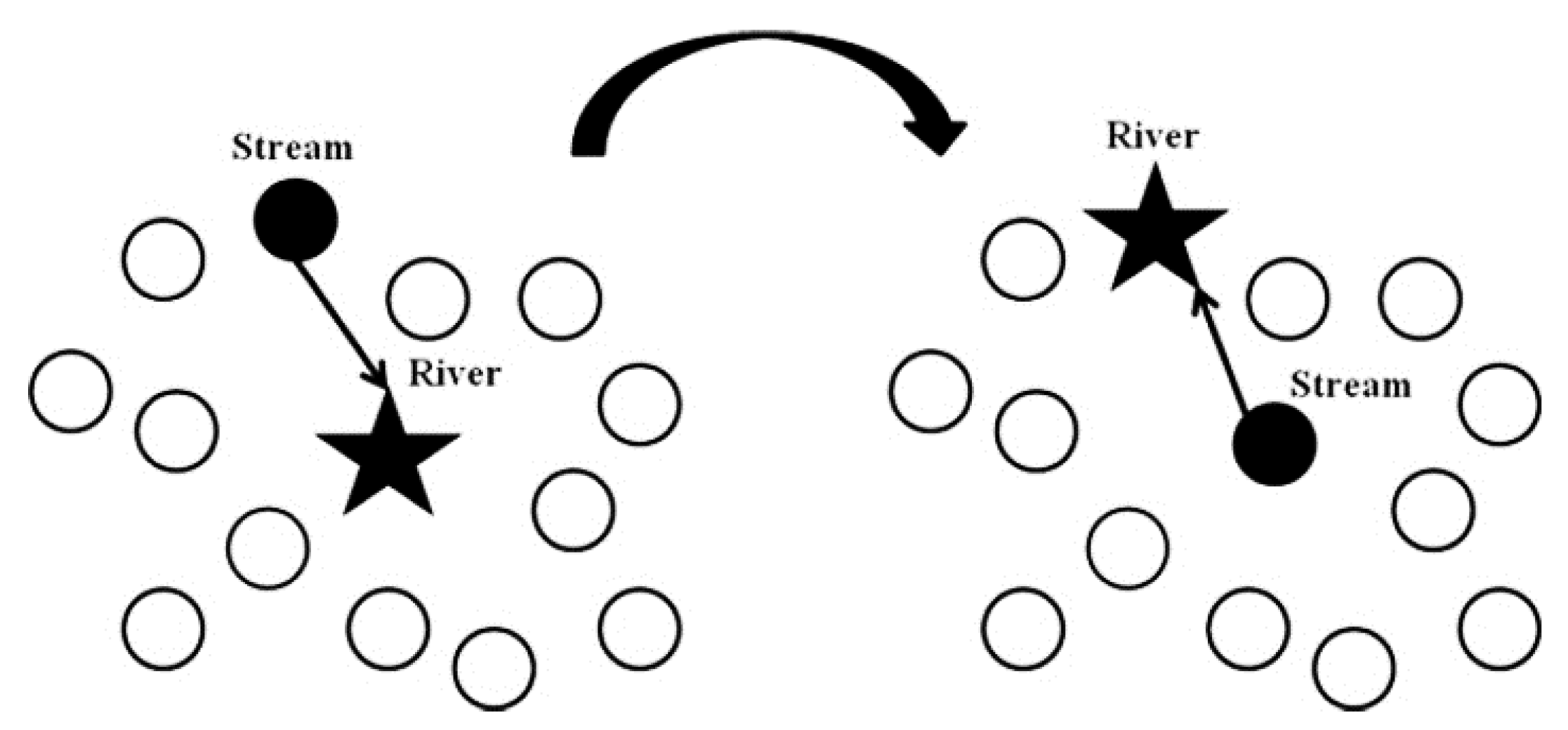
• Step 7: replace the positions of river and stream which achieves the best solution as described in Figure 4.
• Step 8: the same as in step 7, replace the position of river with the sea which achieves the best solution. The river may provide a better solution than the sea as described in Figure 4.
• Step 9: review the evaporation condition which can be obtained from the pseudo code.
• Step 10: after the evaporation condition is attained, the precipitation process will start by using Equations (21) and (22).
• Step 11: decrease d_max by using Equation (20).
• Step 12: if the termination criteria are satisfied, the algorithm will be ended. Otherwise, return back to step 5.

The previous procedures are summarized in the flowchart of the water cycle optimization algorithm illustrated in Figure 5.

GA is a well-known meta-heuristic technique. GA has been applied to different engineering technical problems. GA simulates the Darwin theory based on mating, crossover, and mutations. To keep the best chromosome or generation, the elite criteria must be taken into consideration to keep the best qualities. The WCOA results will be compared to GA results. Figure 6 shows the flowchart of the Genatic Algorithm Technique.

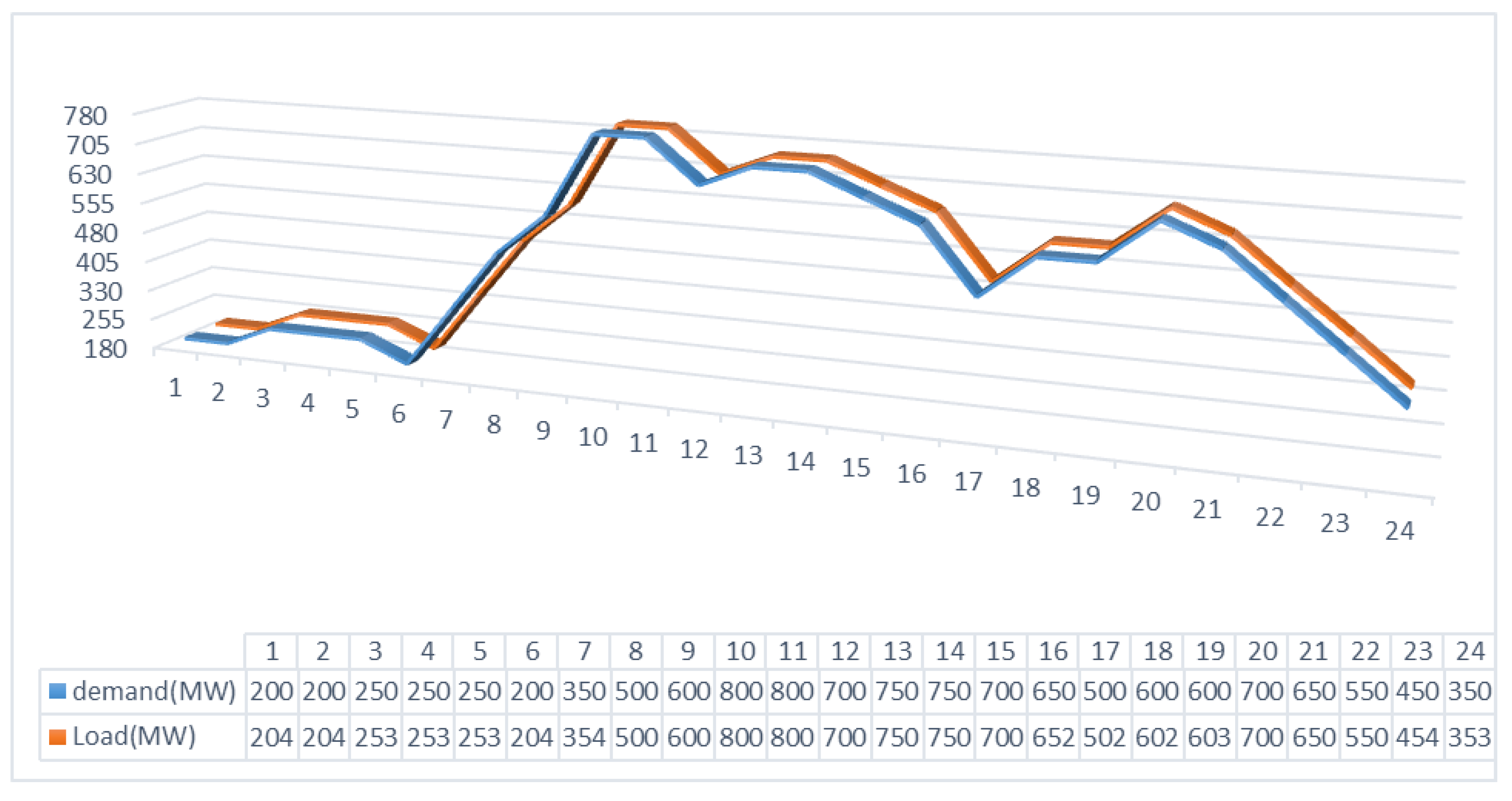
4. System Data under Study and Discussion

A flowchart for minimizing the objective function using thermal (coal-fired) generating units, PEVs and RERs to achieve reduction in both operating cost and support the decarbonization in smart grid through T = 24 h is shown in Figure 7.

An independent system operator “ISO is designed of a single bus test system” which consists of three thermal units designed for simulation with 5000 PEVs and RERs. Thermal generating units are coal-fired due to their low operational costs; and the heat rates of (coal-fired) thermal units are typically in the range of 9000 Btu/kWh to 11,000 with (fuel price = 1 $/MBtu). The thermal power plant data is described and collected from [40] in

Table 2. Generator data.

Unit	Pmin (MW)	Pmax (MW)	Ramp up (MW/h)	Ramp down (MW/h)	Intial State at Time
G1	30	600	200	50	On
G2	30	600	200	20	Off
G3	20	400	200	50	On

and

Table 3. Generator energy data.

Unit	Fuel Consumption Function			Startup Cost ($)	Shut down Cost ($)
	A (MBtu)	B (MBtu/MWh)	C (MBtu/MWh2)
G1	176.9	13.5	0.04	1200	800
G2	129.9	40.6	0.001	1000	500
G3	137.4	17.6	0.005	1500	800

. Wind and solar power plants in this model are described in

Table 4. Wind–solar energy.

Hour	Wind (MW)	Solar (MW)	Hour	Wind (MW)	Solar (MW)	Hour	Wind (MW)	Solar (MW)	Hour	Wind (MW)	Solar (MW)
1	8.2	0	7	4.6	5	13	59.0	65.0	19	72.2	0
2	11.4	0	8	49.3	22.04	14	78.1	58.27	20	73.3	0
3	66.9	0	9	45.6	53.95	15	44.9	53.79	21	65.3	0
4	69.8	0	10	10.1	67.4	16	19.5	47.06	22	24.5	0
5	55.4	0	11	24.8	67.32	17	3.7	27.11	23	49.9	0
6	50.9	0	12	37.3	69.64	18	16.5	11	24	40.3	0

and data is collected from [41].

The parameters of a random model of PEVs are: Expected total number of PEVs in the smart grid = 5000; Maximum capacity of the battery = 25 kWh; Minimum capacity of the battery = 10 kWh; Average capacity of the battery “Pavg” = 15 kWh; Frequency of charging/discharging =1 per day; Departure state of charge (SOC) “Ψ_dep” = 50%; Efficiency “η” = 85%. A typical PEV needs about 8.22 kWh/day (41.1 MWh/day) for 5000 vehicles, 2.6 $/gallon (fuel price = 1 $/MBtu) for gasoline price taking into consideration the emission factor for fuel oil from Table 1, assuming the scenario for simulation of PEVs according to the demand which is relatively low during hours 1–7, 16–19 and 23–24 (a total of 12 h). PEVs can be charged during the off-peak load. Therefore, an additional 41.1 MWh load for 5000 vehicles assuming the number of vehicles will be charged for each hour in Figure 8 [41].

Costs for wind and solar energy are estimated by the International Renewable Energy Agency (IRENA). The levelized cost of electricity (LCOE) from solar photovoltaics (PV) fell by 69% between 2010 and 2017 reaching the cost range of fossil fuels. Wind costs fell by 15% in the same period. For solar energy (14.597 $/MW) and wind energy (10 $/MW) [42].

5. Simulation Results

The parameters for the proposed algorithm (WCOA): N_pop = 70, N_sr = 3 (2 rivers + 1 sea), dmax = 10⁻⁵, max_iteration = 700, assuming the spinning reserve is a minimum of 10% of the load demand condition. Four cases are being considered and the results from the proposed algorithm (WCOA) are compared with Genetic Algorithm (GA) and Dynamic Programming (DP).

Table 5. Base case of 3 thermal Generating units’ applying the WCOA.

Time (Hour)	ThermUnit-1 (MW)		ThermUnit-2 (MW)		ThermUnit-3 (MW)	Emission (ton)		Demand (MW)
1	67.735		0		132.265	191		200
2	67.778		0		132.222	191		200
3	73.334		0		176.666	238.75		250
4	73.333		0		176.667	238.75		250
5	73.332		0		176.668	238.75		250
6	67.633		0		132.367	191		200
7	84.444		0		265.556	334.25		350
8	101.109		0		398.891	477.5		500
9	92.734		158.375		348.891	573		600
10	97.089		329.012		373.899	764		800
11	96.688		339.075		364.237	764		800
12	66.688		319.075		314.237	668.5		700
13	95.658		299.075		355.267	716.25		750
14	95.126		296.051		358.823	716.25		750
15	92.654		276.051		331.295	668.5		700
16	89.327		256.051		304.622	620.75		650
17	101.11		0		398.89	477.5		500
18	92.677		158.433		348.89	573		600
19	93.117		173.822		333.061	573		600
20	95.146		254.079		350.775	668.5		700
21	91.782		234.08		324.138	620.75		650
22	150		0		400	525.25		550
23	100		0		350	429.75		450
24	50		0		300	334.25		350
Start-up cost		Fuel cost		Total cost			Emissions
3000.000 $/day		247,284.867 $/day		368,227.367 $/day			11,794.250 ton/day

The total production and emission cost for the base three generator units is 368,227.367 $/day.

,

Table 6. Integration PEVs (V2G/G2V) with base 3 thermal generating units’ applying the WCOA.

Time (Hour)	ThermUnit-1 (MW)		ThermUnit-2 (MW)	ThermUnit-3 (MW)		PEV Unit-4 (V2G/G2V)	Emission (Ton)		Demand (MW)
1	68.173		0	135.381		−3.554	194.394		203.554
2	68.174		0	135.342		−3.516	194.358		203.516
3	73.677		0	179.391		−3.068	241.68		253.068
4	73.659		0	179.554		−3.213	241.818		253.213
5	73.531		0	179.481		−3.012	241.626		253.012
6	68.852		0	135.454		−3.624	194.461		203.624
7	84.852		0	268.82		−3.672	337.757		353.672
8	100.221		0	391.791		7.988	477.005		500
9	192.733		0	400		7.268	572.549		600
10	339.856		44.207	400		15.938	763.012		800
11	339.777		41.098	400		19.125	762.814		800
12	289.777		30	364.285		15.938	667.512		700
13	311.075		30	400		8.925	715.697		750
14	306.945		30	400		13.055	715.441		750
15	264.993		30	400		5.007	668.19		700
16	222.242		30	400		−2.242	622.891		652.242
17	0		102.363	400		−2.363	479.756		502.363
18	120.136		82.363	400		−2.499	575.386		602.499
19	202.808		0	400		−2.808	575.681		602.808
20	291.596		0	400		8.404	667.979		700
21	241.596		0	396.849		11.555	620.034		650
22	191.596		0	351.682		6.721	524.833		550
23	141.596		0	312.563		−4.159	433.722		454.159
24	0		0	353.322		−3.322	337.422		353.322
Start-up cost		Fuel cost			Total cost			Emissions
4300.000 $/day		269,843.179 $/day			392,403.355 $/day			11,826.018 ton/day

Note: load is leveled when the load of PEVs (G2V) is added to demand, Positive and negative values indicate V2G/G2V (discharging/charging) respectively.

,

Table 7. Integration of RESs (Wind-Solar) with base three thermal generating units’ simulation results by using the WCOA.

Time (Hour)	ThermUnit-1 (MW)		ThermUnit-2 (MW)	ThermUnit-3 (MW)		Wind (MW)	Solar (MW)		Emission (ton)	Demand (MW)
1	66.867		0	124.933		8.2	0		183.341	200
2	66.511		0	122.089		11.4	0		180.352	200
3	65.901		0	117.119		66.9	0		176.265	250
4	65.578		0	114.622		69.8	0		173.557	250
5	67.178		0	127.422		55.4	0		187.006	250
6	62.122		0	86.978		50.9	0		143.459	200
7	83.378		0	257.022		4.6	5		325.209	350
8	93.132		0	335.528		49.3	22.04		410.538	500
9	101.16		0	399.29		45.6	53.95		479.211	600
10	292.5		30	400		10.1	67.4		690.604	800
11	277.88		30	400		24.8	67.32		676.95	800
12	0		193.06	400		37.3	69.64		567.573	700
13	0		226	400		59	65		599.459	750
14	0		213.63	400		78.1	58.27		588.006	750
15	57.68		193.63	350		44.9	53.79		575.517	700
16	183.44		0	400		19.5	47.06		557.877	650
17	133.44		0	362.86		3.7	0		474.044	500
18	172.8		0	400		16.5	11		547.15	600
19	127.8		0	400		72.2	0		505.565	600
20	226.7		0	400		73.3	0		600.038	700
21	184.7		0	400		65.3	0		559.76	650
22	134.7		0	390.8		24.5	0		502.367	550
23	95.556		0	354.444		0	0		429.75	450
24	45.556		0	304.444		0	0		334.25	350
Start-up cost		Fuel cost			Total cost			Emissions
4800.000 $/day		257,120.030 $/day			366,598.528 $/day			10,467.850 ton/day

and

Table 8. Integration PEVs with RESs (wind-solar) with base three thermal generating units’ simulation results by the WCOA.

Time (Hour)	Therm Unit-1 (MW)	Therm Unit-2 (MW)		Therm Unit-3 (MW)	PEV Unit-4 (V2G/G2V)(MW)		Wind (MW)	Solar (MW)		Emission (Ton)	Demand (MW)
1	67.262	0		128.092	−3.554		8.2	0		186.735	203.554
2	66.902	0		125.214	−3.516		11.4	0		183.71	203.516
3	66.283	0		119.885	−3.068		66.9	0		179.195	253.068
4	65.855	0		117.558	−3.213		69.8	0		176.625	253.213
5	67.511	0		130.1	−3.012		55.4	0		189.882	253.012
6	62.524	0		90.2	−3.624		50.9	0		146.92	203.624
7	83.785	0		260.287	−3.672		4.6	5		328.715	353.672
8	92.344	0		328.328	7.988		49.3	22.04		410.043	500
9	100.351	0		392.831	7.268		45.6	53.95		478.76	600
10	276.563	30		400	15.938		10.1	67.4		689.616	800
11	258.755	30		400	19.125		24.8	67.32		675.764	800
12	0	177.123		400	15.938		37.3	69.64		566.585	700
13	96.516	157.123		363.437	8.925		59	65		598.906	750
14	97.064	137.123		366.389	13.055		78.1	58.27		587.197	750
15	196.303	0		400	5.007		44.9	53.79		575.206	700
16	185.682	0		400	−2.242		19.5	47.06		560.018	652.242
17	0	71.553		400	−2.363		3.7	27.11		450.573	502.363
18	123.446	51.553		400	−2.499		16.5	11		549.536	602.499
19	101.006	31.553		398.049	−2.808		72.2	0		508.246	602.808
20	188.296	30		400	8.404		73.3	0		599.517	700
21	143.145	30		400	11.555		65.3	0		559.043	650
22	99.866	30		388.913	6.721		24.5	0		501.95	550
23	65.346	0		338.913	−4.159		49.9	0		387.115	454.159
24	64.409	0		288.913	−3.322		0	0		337.422	353.322
Start-up cost			Fuel cost			Emissions			Total cost
7100.000 $/day			251,804.935 $/day			10,427.283 ton/day			363,177.769 $/day

Note: load is leveled when the load of PEVs (G2V) is added to demand, Positive and negative values indicate V2G/G2V (discharging/charging) respectively.

below explain applying the WCOA. The whole comparison of the three applied techniques DP, GA, and WCOA is shown in

Table 9. Results summary for WCOA, GA and DP (including emission cost).

Algorithm	Modes	Start-Up Cost ($/Day)	Production Cost ($/Day)	Total Cost (Including Emission Cost) ($/Day)	Emissions (Ton/Day)
WCOA	Base 3 thermal units	3000	247,284.867	368,227.367	11,794.250
	PEVs(V2G/G2V) with 3 thermal units	4300	269,843.179	392,403.355	11,826.018
	RESs with 3-thermal units	4800	257,120.30	366,598.528	10,467.850
	PEVs(V2G/G2V), RESs with 3-thermal units	7100	251,804.935	363,177.769	10,427.283
GA	Base 3 thermal units	3000	247,284.949	368,227.222	11,794.227
	PEVs(V2G/G2V) with 3 thermal units	4300	272,676.166	395,270.780	11,829.461
	RESs with 3-thermal units	4800	264,149.704	376,118.886	10,716.918
	PEVs(V2G/G2V), RESs with 3 thermal units	4400	258,840.379	367,602.876	10,436.250
DP	Base 3-thermal units	3000	247,281.115	368,223.615	11,794.250
	PEVs(V2G/G2V) with 3 thermal units	4300	270,155.998	392,716.173	11,826.018
	RESs with 3-thermal units	4800	257,120.030	366,598.528	10,467.850
	PEVs(V2G/G2V), RESs with 3 thermal units	7100	251,804.939	363,177.773	10,427.283

.

5.1. Case 1 (Base Case)

Case 1 illustrates the distribution of the unit commitment scheduling for the three thermal units only as shown in Table 5.

5.2. Case 2 (PEVs and Three Thermal Units)

PEVs represent one of the newly added techniques to gain energy to support the network. Many strategies were investigated, and most of them agreed on applying PEVs to reduce small fluctuations and improve quality [41]. Case 2 represents the unit commitment after integrating 5000 PEV (V2G/G2V) with the three thermal units, as shown in Table 6.

By comparing both Table 6 and Table 7, start-up, production cost, and emission increase when integrating PEVs with the base case three thermal units by 1300 $/day; 22,558.31 $/day and exceeding the emission by 31.768 ton/day from the coal-fired generators to supply energy to PEVs and emissions from PEV_S 90.7441 ton/day (33,121.597 ton/year for 5000 vehicles) in the transportation sector [34].

5.3. Case3 (RERs, and Three Thermal Units)

Integrating RERs, both wind and solar energy to partially replace thermal (coal-fired) generation units will contribute to reduction in both the production and the emission cost. However, production costs of wind and solar energy resources are relatively high; and the operation and maintenance prices are significantly decreasing. This encourages the usage of these energy resources that also support decarbonizing in the smart grid. Case 3 signifies the unit commitment after integrating RERs (wind & solar), with the three thermal units, as shown in Table 7.

Integrating both RERs and PEVs into the smart grid showed a significant decrease in fuel cost, emissions and total cost which fell to 5,315.365 $/day, 40.567 ton/day; 3,420.759 $/day as compared to integrating RESs with the three thermal units which led to decrease to 18,038.244 $/day, 1,398.735 ton/day, 29,225.586 $/day and compared to integrating PEVs into the three thermal units.

5.4. Case 4 (RERs, PEVs, and the Three Thermal Units)

RERs are accumulated to reduce emissions from both conventional units and PEVs. On the other hand, PEVs are integrated to solve the uncertainty behavior of RERs. Therefore, further enhancement for the reliability and stability of the grid can be covered up against any unexpected uncertainty behavior for RESs by including the grid for both the integration of RES and PEVs. Case 4 implies the unit commitment after integrating RERs (wind & solar), 5000 PEV (V2G/G2V) with the 3 thermal units, as shown in Table 8.

Comparing the results obtained from the proposed algorithm (WCOA) with the results obtained from the forward dynamic programming (DP) and genetic algorithm (GA) as shown in Table 9 including the emission and emission cost.

Table 9 sums up the whole comparison between the results obtained from the proposed algorithm (WCOA) with the results obtained from (DP) and (GA). Table 9 provides three main outcomes. First, the power of the WCOA in solving the unit commitment problem indicated in the yellow boxes. Second, the green box shows that the emission cost slightly increased integrating combined PEVs but with the existence of PEVs to support wind and solar units. So the need to pay more attention and facilities to invest in the PEVs (electrically based) will lead to more reduction in the emission costs. Third, focusing on the production cost in any case aims to lower the price to 2/3 of its price, but this will increase cost on the long term operation.

6. Discussion

The above mentioned tables can be summed up as follows:

• The total cost and emissions for the base 3-generator units increase when integrating PEVs with the base 3 thermal units, and exceed the emission limit more than the base case.
• Integrating RERs, both wind and solar energy to partially replace thermal (coal-fired) generation units contributes to reducting both the fuel cost and the emissions. Significant reduction in emission occurs when integrating only RERs with the base three thermal units. However, the uncertainty of wind and solar energy is based on several factors such as geographical area, the forecasting models used and period-ahead forecasting. These variables affect the uncertainty percentage and the overall accuracy.
• Integrating both RERs and PEVs into the smart grid showed a significant decrease in fuel cost, emissions and total cost. RERs is accumulated to reduce emissions from both conventional units and PEVs. PEVs is integrated to solve the uncertainty behavior of RERs.
• The results extracted from the proposed algorithm (WCOA) proved its efficiency with respect to the results of both dynamic programing (DP) and genetic algorithm (GA).

7. Conclusions

In this paper, the unit commitment problem has been solved in four different modes with three algorithms, provided with results and analysis to achieve;

(i)

Reduction in total cost including the emission cost.

(ii)

Decarbonizing the emissions from the conventional generators and the transportation sector.

(iii)

Presenting new types of storage energy in the electricity sector by replacing conventional vehicles with electrical vehicles with environment-friendly batteries and encouraging the consumers to supply electrical power to the grid during the on-peak periods.

The four modes are;

(1)

The base 3-thermal (coal-fired) units.

(2)

PEVs (V2G/G2V) with the conventional units.

(3)

RERs (wind/Solar) with the conventional units.

(4)

Integrating PEVs (V2G/G2V), RERs (wind/solar) with the conventional units.

The four modes are executed applying three algorithms which are;

(1)

Water cycle optimization algorithm (WCOA).

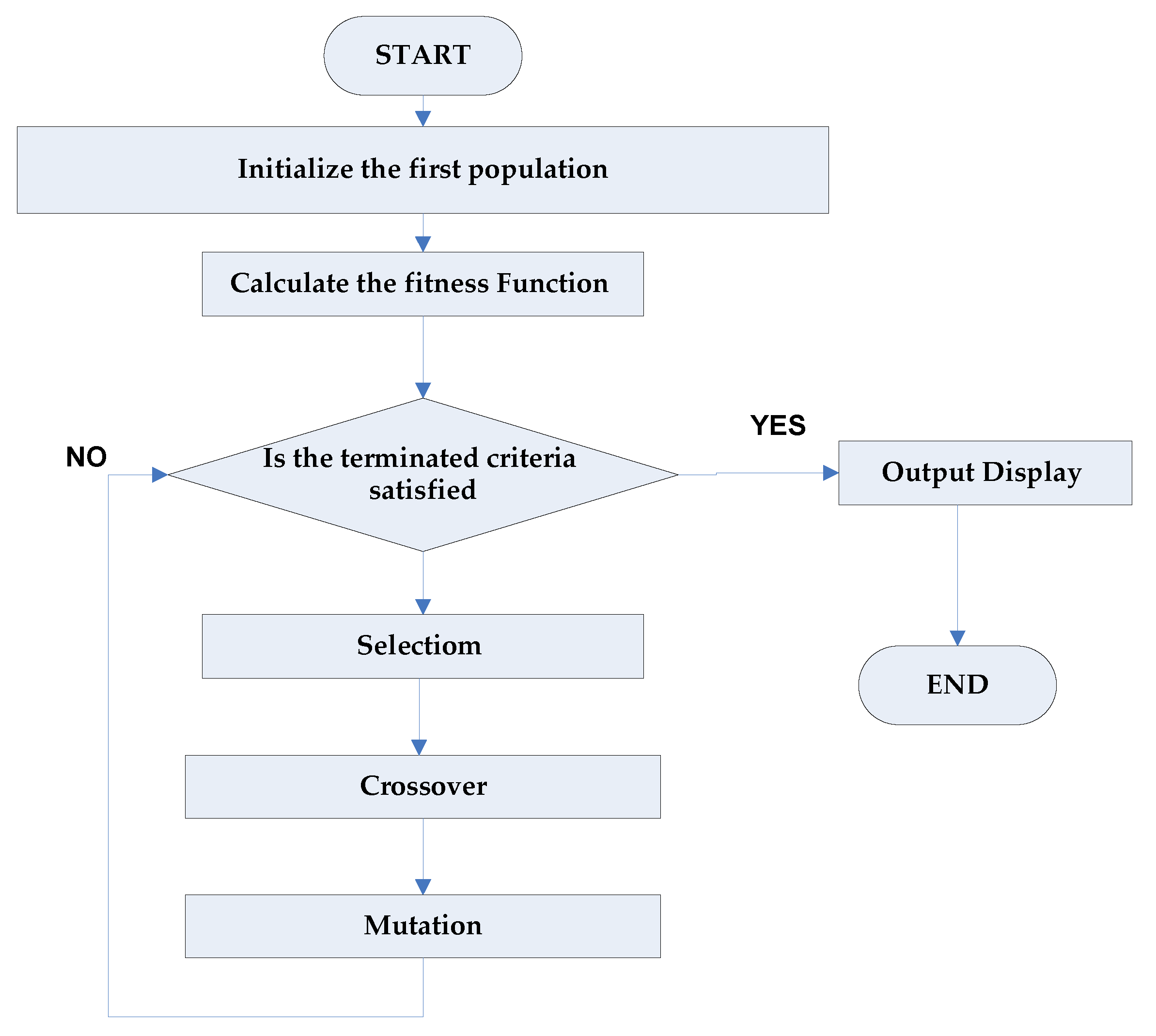
(2)

Genetic algorithm (GA).

(3)

Dynamic programing (DP).

Based on the comparison of the proposed technique with other optimization algorithms, WCOA has shown promising performance and better solutions than GA and DP techniques. In the four modes of study, the WCOA offers competitive results with respect to other meta-heuristic optimization techniques with acceptable degree of accuracy for the solutions.

From this study, it is concluded that, integrating both PEVs and RERs with the conventional generating units achieved many purposes;

(i)

Increasing the reliability and stability of the electricity grid.

(ii)

Decarbonizing the emissions from the electricity sector and transportation sector.

(iii)

Introducing new types of unit commitment sourses with different distributions, for environment-friendly electrical energy storage such as PEVs (V2G) to encourage the consumers to supply electrical power to the grid during the on-peak periods of the electrical network operation.

References

1. Lopez, C.J.; Ano, O.; Esteybar, D.O. Stochastic Unit Commitment & Optimal Allocation of Reserves: A Hybrid Decomposition Approach. IEEE Trans. Power Syst. 2018. [Google Scholar] [CrossRef]
2. Krishnamurthy, S.; Tzoneva, R. Comparative analyses of Min-Max and Max-Max price penalty factor approaches for multi criteria power system dispatch problem with valve point effect loading using Lagrange’s method. In Proceedings of the 2011 IEEE International Conference on Power and Energy Systems (ICPS), Chennai, India, 22–24 December 2011. [Google Scholar] [CrossRef]
3. Zhou, B.; Ai, X.; Fang, J.; Wen, J.; Yang, J. Mixed-integer second-order cone programming taking appropriate approximation for the unit commitment in hybrid AC–DC grid. In Proceedings of the IEEE 6th International Conference on Renewable Power Generation (RPG), Wuhan, China, 19–20 October 2017. [Google Scholar]
4. Alejandre, L.M.C.; Alcaraz, G.G. Analysis of Security Constrained Unit Commitment using Three Models of Electricity Generation Cost Linearization. In Proceedings of the IEEE Conference on Texas Power and Energy Conference (TPEC), College Station, TX, USA, 8–9 February 2018. [Google Scholar] [CrossRef]
5. Elsayed, A.M.; Maklad, A.M.; Farrag, S.M. A New Priority List Unit Commitment Method for Large-Scale Power Systems. In Proceedings of the 2017 Nineteenth International Middle East Power Systems Conference (MEPCON), Cairo, Egypt, 19–21 December 2017. [Google Scholar]
6. Venayagamoorthy, G.K.; Braband, G. Carbon reduction potential with intelligent control of power systems. In Proceedings of the 17th World Congress: International Federation of Automatic Control, Seoul, Korea, 6–11 July 2008. [Google Scholar]
7. Labatt, S.; White, R.R. Carbon Finance: The Financial Implications of Climate Change; Wiley: Hoboken, NJ, USA, 2007. [Google Scholar]
8. Godina, R.; Rodrigues, E.M.G.; Pouresmaeil, E.; Catalão, J.P.S. Optimal residential model predictive control energy management performance with PV microgeneration. Comput. Oper. Res. 2017, in press. [Google Scholar]
9. Rodrigues, E.M.G.; Godina, R.; Pouresmaeil, E.; Ferreira, J.R.; Catalão, J.P.S. Domestic appliances energy optimization with model predictive control. Energy Convers. Manag. 2017, 142, 402–413. [Google Scholar] [CrossRef]
10. Oliveira, D.; Rodrigues, E.M.G.; Godina, R.; Mendes, T.D.P.; Catalão, J.P.S.; Pouresmaeil, E. Enhancing Home Appliances Energy Optimization with Solar Power Integration. In Proceedings of the IEEE International Conference on Computer as a Tool (EUROCON 2015), Salamanca, Spain, 8–11 September 2015. [Google Scholar] [CrossRef]
11. Godina, R.; Rodrigues, E.M.G.; Pouresmaei, E.; Matias, J.C.O.; Catalão, J.P.S. Model Predictive Control Home Energy Management and Optimization Strategy with Demand Response. Appl. Sci. 2018, 8, 408. [Google Scholar] [CrossRef]
12. Silva, J.M.; Rodrigues, E.; Godina, R.; Catalao, J.P.S. Residential MPC controller performance in a household with PV microgeneration. In Proceedings of the 2017 IEEE Conference on Manchester PowerTech, Manchester, UK, 18–22 June 2017. [Google Scholar] [CrossRef]
13. Nguyen, D.T.; Le, L.B. Risk-constrained profit maximization for microgrid aggregators with demand response. IEEE Trans. Smart Grid 2015, 6, 135–146. [Google Scholar] [CrossRef]
14. Stock, A.; Stock, P.; Sahajwalla, V. Powerful Potential: Battery Storage for Renewable Energy and Electric Cars; Climate Council of Australia Ltd.: Sydney, Australia, 2015; ISBN 978-0-9944195-4-5 (print), 978-0-9944195-3-8 (web). [Google Scholar]
15. Nieto, A.; Vita, V.; Maris, T.I. Power quality improvement in power grids with the integration of energy storage systems. Int. J. Eng. Res. Technol. (IJERT) 2016, 5, 438–443. [Google Scholar]
16. Nykvist, B.; Nilsson, M. Rapidly falling costs of battery packs for electric vehicles. Nat. Clim. Chang. 2015, 5, 329–332. Available online: http://www.nature.com/nclimate/journal/v5/n4/full/nclimate2564.html (accessed on 12 March 2018). [CrossRef]
17. King Island Advanced Hybrid Power Station. Available online: www.kingislandrenewableenergy.com.au/history/king-island-renewable-energy (accessed on 13 March 2018).
18. Al Ghaithi, H.M.; Fotis, G.P.; Vita, V. Techno-economic assessment of hybrid energy off-grid system—A case study for Masirah island in Oman. Int. J. Power Energy Res. 2017, 1, 103–116. [Google Scholar] [CrossRef]
19. Agamah, S.U.; Ekonomou, L. Energy storage system scheduling for peak demand reduction using evolutionary combinatorial optimization. Sustain. Energy Technol. Assess. 2017, 23, 73–82. [Google Scholar]
20. Agamah, S.; Ekonomou, L. A heuristic combinatorial optimization algorithm for load-leveling and peak demand reduction using energy storage systems. Electr. Power Compon. Syst. 2018, 45, 2093–2103. [Google Scholar] [CrossRef]
21. Center for Climate and Energy Solution. Climate Solution, Technology Solution, Electrical Vehicles. Available online: www.c2es.org/content/electric-vehicles/ (accessed on 3 March 2018).
22. Little, A.D.; Browning, L.; Santini, D.; Vyas, A.; Taylor, D.; Markel, T.; Duvall, M.; Graham, R.; Miller, A.; Frank, A.; et al. Comparing the Benefits and Impacts of Hybrid Electric Vehicle Options; for Compact Sedan and Sport Utility Vehicles; Electric Power Research Institute (EPRI): Palo Alto, CA, USA, 2002; p. 1006892. Available online: http://www.evworld.com/library/EPRI_sedan_options.pdf (accessed on 13 March 2018).
23. Corrigan, D.; Masias, A. Batteries for Electric and Hybrid Vehicles. In Linden’s Handbook of Batteries, 4th ed.; Reddy, T.B., Ed.; McGraw Hill: New York, NY, USA, 2011. [Google Scholar]
24. Vita, V. Development of a decision-making algorithm for the optimum size and placement of distributed generation units in distribution networks. Energies 2017, 10, 1433. [Google Scholar] [CrossRef]
25. Boulanger, A.G.; Chu, A.C.; Maxx, S.; Waltz, D.L. Vehicle electrification: Status and issues. Proc. IEEE 2011, 99, 1116–1138. [Google Scholar] [CrossRef]
26. Ghasemi, A.; Mortazavi, S.S.; Mashhour, E. Hourly demand response and battery energy storage for imbalance reduction of smart distribution company embedded with electric vehicles and wind farms. Renew. Energy 2016, 85, 124–136. [Google Scholar] [CrossRef]
27. Morais, H.; Sousa, T.; Soares, J.; Faria, P.; Vale, Z. Distributed energy resources management using plug-in hybrid electric vehicles as a fuel-shifting demand response resource. Energy Convers. Manag. 2015, 97, 78–93. [Google Scholar] [CrossRef]
28. Li, K.; Xue, Y.; Cui, S.; Niu, Q.; Yang, Z.; Luk, P. Advanced computational methods in energy, power, electric vehicles and their integration. In Proceedings of the International Conference on Life System Modeling and Simulation (LSMS2017) and International Conference on Intelligent Computing for Sustainable Energy and Environment (ICSEE 2017), Nanjing, China, 22–24 September 2017; Part III. Springer: Berlin, Germany, 1842. [Google Scholar]
29. Wedyan, A.; Whalley, J.; Narayanan, A. Hydrological Cycle Algorithm for Continuous Optimization Problems. J. Glob. Optim. 2017, 37, 405–436. [Google Scholar] [CrossRef]
30. Moradi, M.; Sadollah, A.; Eskandar, H.; Eskandarc, H. The application of water cycle algorithm to portfolio selection. J. Econ. Res. Ekon. Istraž. 2017, 30, 1277–1299. [Google Scholar]
31. Yanjun, K.; Yadong, M.; Weinan, L.; Xianxun, W.; Yue, B. An enhanced water cycle algorithm for optimization of multi-reservoir systems. In Proceedings of the 2017 IEEE/ACIS 16th International Conference on Computer and Information Science (ICIS), Wuhan, China, 24–26 May 2017. [Google Scholar]
32. Eskandara, H.; Sadollahb, H.; Bahreininejadb, A. Weight Optimization of Truss Structures Using Water Cycle Algorithm. Int. J. Optim. Civ. Eng. 2013, 3, 115–129. [Google Scholar]
33. Sadollah, A.; Eskandar, H.; Kim, J. Water cycle algorithm for solving constrained multi-objective optimization problems. Appl. Soft Comput. 2015, 27, 279–298. [Google Scholar] [CrossRef]
34. World Bank and Ecofys. Carbon Pricing Watch 2017. 2017. Available online: https://openknowledge.worldbank.org/handle/10986/26565, (accessed on 3 March 2018).
35. Tung, N.S.; Bhadoria, A.; Kaur, K.; Bhadauria, S. Dynamic programming model based on cost minimization algorithms for thermal generating units. Int. J. Enhanc. Res. Sci. Technol. Eng. 2012, 1, 19–27. [Google Scholar]
36. Thakur, N.; Titare, L.S. Determination of unit commitment problem using dynamic programming. Int. J. Nov. Res. Electr. Mech. Eng. 2016, 3, 24–28. [Google Scholar]
37. Shi, J.; Dong, X.; Zhao, T.; Du, Y.; Liu, H.; Wang, Z.; Zhu, D.; Xiong, C.; Jiang, L.; Shi, J.; et al. The Water Cycle Observation Mission (WCOM): Overview. In Proceedings of the IEEE International Geoscience and Remote Sensing Symposium (IGARSS), Beijing, China, 10–15 July 2016. [Google Scholar]
38. Bozorg-Haddad, O.; Solgi, M.; Loáiciga, H.A. Meta-Heuristic and Evolutionary Algorithms for Engineering Optimization, 1st ed.; John Wiley & Sons, Inc.: Hoboken, NJ, USA, 2017; pp. 231–240. [Google Scholar]
39. Eskandar, H.; Sadollah, A.; Bahreininejad, A.; Hamdi, M. Water cycle algorithm—A novel metaheuristic optimization method for solving constrained engineering optimization problems. Comput. Struct. 2012, 110–111, 151–166. [Google Scholar] [CrossRef]
40. He, D.; Tan, Z.; Harley, R.G. Chance constrained unit commitment with wind generation and superconducting magnetic energy storages. In Proceedings of the IEEE Power and Energy Society General Meeting, San Diego, CA, USA, 22–26 July 2012. [Google Scholar]
41. Saber, A.Y.; Venayagamoorthy, G.K. Efficient utilization of renewable energy sources by gridable vehicles in cyber-physical energy systems. IEEE Syst. J. 2010, 4, 285–294. [Google Scholar] [CrossRef]
42. International Renewable Energy Agency (IRENA). Renewable Power Generation Costs in 2017; International Renewable Energy Agency: Abu Dhabi, United Arab Emirates, 2018; Available online: http://www.irena.org/publications/2018/Jan/Renewable-power-generation-costs-in-2017 (accessed on 18 March 2018).
Figure 1. A flowchart for the forward dynamic programming algorithm.
Energies 11 01140 g001
Figure 2. A simplified diagram of the water cycle (the hydrologic cycle) [37].
Energies 11 01140 g002
Figure 3. Schematic view for water cycle algorithm [38].
Energies 11 01140 g003
Figure 4. The position of the stream (raindrop) and the river replacement [38]. The star is the river and the black circle is the best among other streams.
Energies 11 01140 g004
Figure 5. A flowchart for water cycle optimization algorithm.
Energies 11 01140 g005
Figure 6. A flowchart of GA.
Energies 11 01140 g006
Figure 7. A flowchart for minimizing both cost and emission by using PEVs and RERs.
Energies 11 01140 g007
Figure 8. Load leveling for PEVs. Note: The PEVs is integrated as load for the whole day except from hour 8 till hour 15 and from hour 20 till hour 22.
Energies 11 01140 g008