Abstract
With ever increasing demand for electricity and the huge potential of renewable energy, an increasing number of renewable-energy sources are being used to generate electricity. However, due to the intermittency of renewable-energy generation, many researchers try to overcome the variable nature of renewable energy. A hybrid renewable-energy system is one possible way to introduce smoothing of the supply. Many hybrid renewable-energy studies focus on system optimization and management. This paper mainly researches the performance prediction accuracy of a hybrid solar and wind system. Through a mixed autoregressive and dynamical system model, we test the predictability of the hybrid system and compare it with individual solar and wind series forecasting. After error analysis, the predictability of the hybrid system shows a better performance than solar or wind for Adelaide global solar radiation and Starfish Hill wind farm data. The prediction errors were reduced by 13% to more than 30% according to various error analyses. This result indicates an advantage of the hybrid solar and wind system compared to solar and wind systems taken individually.
1. Introduction
Taking into account ever increasing energy consumption, as well as the exhaustible nature of conventional energy sources and the increasingly serious greenhouse effect, special attention has been focused on renewable-energy sources. Solar and wind are the most promising and widely used renewable-energy sources in the world. However, there is no solar radiation during the night and sometimes no wind on a sunny day. In recent studies, most researchers have focused on mainly four research areas. The first area corresponds to renewable-energy policy which establishes the regulations for enhancing the use of renewable energy in several regions, countries or different energy-supply sources to complement each other [1,2,3] or for instance sets diesel fuels as the main sources of renewable energy plants for mini stand-alone grid systems in order to save money and have fewer environmental effects [4,5]. A second area is the utilization of wind and solar energy to generate other storable energy carriers, such as hydrogen [6] or to transform electricity generated by renewable sources to other types of energy, such as a pumped storage system [7]. For the last two areas, there is also the use of the observed wind and solar farm output or simulated data series, as well as a storage system to investigate modeling for grid-connected [8,9,10,11,12] or stand-alone [13,14,15,16,17,18] systems to meet demand.
This paper will focus on one aspect of the last two research areas by discussing data modeling and forecasting. Many researchers focus on modeling and establishing a hybrid solar and wind system to overcome their individual faults and enhance their positive effect on the environment. The last two research areas of modeling hybrid solar and wind for grid-connected and stand-alone systems, in terms of the goal of research, usually targets adaptation of demand to supply or a search for an economic optimum. Of course, these two different research directions also intersect each other according to research targets. Grid-connected renewable-energy system modeling usually intersects with both demand and finance. Based on the Monte Carlo methods, Vasilj, J. et al. [19] simulate the wind speed, the solar radiation and error simulation to construct a system model. Then, the model is used to balance demand and supply. The ultimate goal is to plan future new wind and solar farms. Peng C. et al. [20] proposed a novel ultra-short-term pre-plan power curve-based smoothing control approach to model wind–solar–battery power and obtain a maximum renewable energy utilization rate and constrain the use of the battery. This paper is a typical model of an optimization solution for grid-connected renewable-energy systems. Akram et al. [21] show an example of a typical optimization method for the purpose of maximizing economic benefits. Through maximum reliability and minimum cost, they use two constraint-based iterative search algorithms to perform optimal sizing of the wind turbine, solar photovoltaic and storage systems. Hybrid renewable-energy systems in the stand-alone scenario have primary constraint conditions that are the reliability of supply rather than optimized system size or cost. In a review paper [16], the authors indicated that in many studies for isolated renewable-energy supply, system optimization is used to reduce the dependence on conventional energy, such as diesel fuel, by using hybrid renewable energy and storage. Whether it is using the conventional energy or storage system, the main purpose is to maintain the stability of electricity supply. Petrakopoulou et al. [22] perform exergy analysis and simulation of solar and wind power plants to achieve energy autonomy for a Mediterranean island. In their study, to meet the demand of a small island, they use a concentrating solar power plant as a storage system to ensure the stability of the power supply. This also confirms the concept that the stability of the energy supply is a significant goal for setting up a renewable energy system in a stand-alone system scenario. Murat [23] introduced a hybrid system for a small-scale desalination system. The system, through the integration of wind, solar, diesel and storage, determines the proportion of the components based on the optimal economy in an off-grid remote area. With high potential solar and wind sources, the author believes that using a hybrid power system for a reverse osmosis system could be economical for remote areas.
From this introduction, we can see that the study of hybrid renewable-energy systems, whether they are grid-connected or stand-alone, is quite broad. Many papers focus on system integration, stability and economic benefits. However, the accuracy of forecasting renewable energy is equally important for hybrid systems from the point of view of the instability of renewable energy. Quan et al. [24] introduced a hybrid forecasting model based on the artificial neural network (ANN) method for forecasting solar and wind data. Zhang et al. [25] developed a calculation process by using a group of models in a fuzzy algorithm process to obtain an optimal forecasting solution for hourly wind data. Of course, there are a lot of wind and solar prediction studies, but there are not many papers that consider combined wind and solar. Therefore, our previous study of a coupled autoregressive and dynamical system (CARDS) model is used as benchmark model here to test the predictive performance of a hybrid solar and wind system. Note that in the Australia electricity market renewable-energy forecasting is more focused on short time scale prediction information (5 min to 30 min). Models based on time-series methods are more suitable than computer self-learning such as artificial neural networks, and genetic and fuzzy algorithms, for forecasting short time-scale data [26]. Also, time-series methods can provide a stabilized and much faster result for the system. In the case of rapidly required output, there is no need to worry about the convergence of the results given by the time-series methods, because, with the seasonal effects removed, the resulting time series is stationary. Thereafter, using Box–Jenkins methods, a stable forecasting model is ensured. At the same time, the CARDS model has been proved to have reasonable prediction accuracy for short time-scale data. This is the reason why we chose CARDS model as the benchmark model for the paper.
The article will study the advantages of a hybrid solar and wind system from the perspective of predictability. The first section is short-term forecasting by using a coupled an autoregressive and dynamical system (CARDS) model [26] for a simulated solar system. Then, a modified CARDS model is used for real wind farm output data. Thereafter, the CARDS model used for forecasting a hybrid solar and wind system will be discussed. In the next section, error analysis is used for testing the model results, and the conclusion will be addressed at the end.
2. Hybrid Solar and Wind-Prediction Performance Analysis
The research direction of this paper is prediction accuracy under the combination of solar and wind energy systems. In essence, the optimal solution of a hybrid wind and solar energy system does not affect the accuracy of the prediction. Based on Lazard’s latest annual levelized cost of energy analysis [27], the mean value cost of wind and solar energy is 0.045 and 0.05 American dollars per kilowatt hour (kWh), respectively. Those two costs of generating electricity are growing progressively smaller, and eventually the unit generating cost of solar energy may be same or even less than that of wind energy. Therefore, we can assume that the unit cost of wind and solar energy can be regarded as the same. The purpose of setting this assumption is to simplify the problem to avoid discussing the proportions of wind and solar, because the problem of proportions does not affect the performance of predictability of the hybrid solar and wind system. Based on this assumption, we use double the capacity of Starfish Hill wind farm, or installing the same capacity of solar panels from a prediction point of view, to determine the best choice. Under this assumption, the following sections will deal with the set-up for testing the predictability of wind, solar and a hybrid of these.
2.1. Data
The Starfish Hill wind farm energy output and Adelaide Airport measured global solar radiation from August 2009 to January 2010; 30 min of data were used to demonstrate how the CARDS model [27] was employed for prediction performance of a hybrid solar and wind system. Starfish Hill wind farm is near Cape Jervis, South Australia, approximately 88 km south of Adelaide. Adelaide is the capital of South Australia, latitude 34°51′ S, longitude 138°33′ E and the time zone is AEST (UTC+9.5). The wind farm data set consists of 8784 (48 × 183) half-hourly wind power output values in total. The Starfish Hill wind farm installed capacity is 34.5 MW. The wind farm is located south of Adelaide at latitude 35°34′ S and longitude 138°9′ E. The average half-hourly wind-power output was 5.4 MW and the maximum value was 16.9 MW. The solar data set consists of 8784 (48 × 183) half-hourly global radiation values in total. The average half-hourly global radiation was 258 W/m2 including the night-time period, and the maximum value was 1139 W/m2. In order to correspond to the same installed capacity of the Starfish Hill wind farm of 34.5 MW, and according to the Adelaide Airport-measured global solar radiation 30-min data, the energy flow of assumed solar power plant is illustrated in Figure 1. The installed capacity of the solar farm is 34.5 MW, the measured solar panels area about 202,941 m2, and the efficiency rate of solar panels about 17%. Note that the two locations are sufficiently close to be able consider them as a combined solar and wind system, as though the total output feeds into the grid through a single connection. Table 1 displays the Starfish Hill wind farm and assumed solar farm energy output general information.
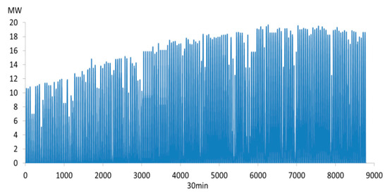
Figure 1.
Energy flow of assumed 34.5 MW-capacity solar farm.

Table 1.
Wind farm and assumed solar farm energy output data information.
2.2. The Coupled Autoregressive and Dynamical System (CARDS) for Solar
The CARDS model is built on the Fourier series, autoregressive (AR) methods, a dynamical system model known as the Lucheroni model [28], and a fixed component [26]. The Lucheroni model is a resonating model for the power market which exploits the simultaneous presence of a Hopf critical point, periodic forcing and noise in a two-dimensional first order non-autonomous stochastic differential equation system for the log price and the derivative of the log price. The fixed component is a variable construct in our previous paper for considering measured data at time t and t − 1 to further correct the problem of the model change delay.
Here, a Fourier series is mainly used to capture the periodic change characteristics of data, which is the non-linear part. The autoregressive component is used to model the linear part of the data. The Lucheroni model is also used to capture the high-frequency part of the data, and the fixed component is used to further improve the accuracy of the linear part. The CARDS model is built by using the Visual Basic® program (VB is a universal object-based programming language developed by Microsoft®).
The first step is using the Fourier series to deseason the data. Following [29], and using the results of Power Spectrum analysis, the Fourier series can be written as St, and the result is shown in Table 2.
Table 2.
Fourier series model in assumed 34.5 MW-capacity solar farm energy-flow data.
Here, is the mean of the data, and are coefficients of the yearly cycle, and and are coefficients of the daily cycle and its harmonics, n and associated beat frequencies, m. Table 1 shows the frequency of yearly, daily and twice-daily cycles, with the percentage of variance of the original time series explained by the contribution of the Fourier series component at each frequency. All significant values are indicated in bold. From Table 1, it can easily be seen that, overall, the St can represent over 80% of the variance of the data. Figure 2 displays the three-day Fourier series compared with assumed solar farm energy-flow data.
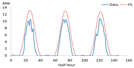
Figure 2.
Three days St compared with the data.
According to the CARDS model steps, the next step is to model the deseasoned data Rt, where is assumed solar farm energy flow based on Adelaide airport-measured global solar radiation 30-min data.
The Box–Jenkins methodology comprises a joint investigation of the sample autocorrelation coupled with the partial autocorrelation function. See Boland [30] for details on how a slowly decaying autoregressive function and a partial autocorrelation function having the bars going to zero abruptly indicate an autoregressive process. Figure 3 shows that the deseasoned data follow a typical AR(2) model, so can be written as,
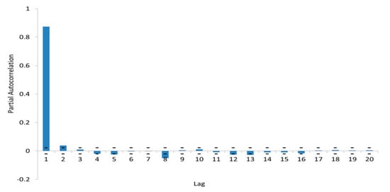
Figure 3.
Partial autocorrelation function for deseasoned data.
Figure 4 shows AR(2) as compared with deseasoned data. Figure 4 shows that the AR(2) cannot capture the maximum value of high-frequency data very well. Therefore, the Lucheroni model is used to make up for the AR model [26,28].
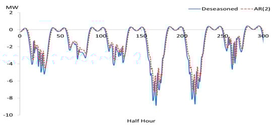
Figure 4.
Shows AR(2) is compared with deseasoned data.
Based on that, the model can be written as,
Here, is the noise after a model is developed for and for forecasting we do not include it in the Lucheroni model, and is Lucheroni model forecast. is time span, which for our data is 1/48, because it corresponds to half-hourly data. The new component is introduced to help us find the future vale of . The ordinary least squares (OLS) is used to estimate all the other components к, λ, ε, γ and b. The coefficients are к = −8.41, λ = −0.94 × 10⁻¹⁵, ε = 0.15, γ = −0.0096 and b = 2.68. Figure 5 shows that the Lucheroni model captures the peak value better than the AR model (compared with Figure 4). Therefore, the Lucheroni model is used for capturing the rising part of residual solar radiation values and AR(2) for falling values. After combining the AR and Lucheroni models, the fixed component is used to further improve the accuracy of the combined AR and Lucheroni model (for more detail see [26]).
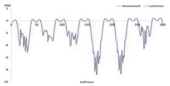
Figure 5.
Lucheroni model compared with deseasoned data.
Based on three different models and one component, the general function of the CARDS and Fourier series models can be written as,
Here, et is assumed to be white noise with mean zero and variance . Equation (6) shows that the Fourier series is used to capture the seasonal component of the data; the combined AR and Lucheroni model is used for the linear part which is the deseasoned component of the data; and the fixed component is used to further improve the forecasting accuracy by modifying the forecasting of the combined AR and Lucheroni model.
Figure 6 shows the three-day Fourier series model plus CARDS model compared with measured Adelaide airport global solar radiation 30-min data generating an assumed energy flow of a solar power plant.
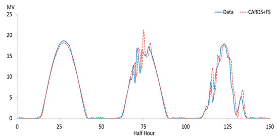
Figure 6.
The three-day coupled autoregressive and dynamical system (CARDS) plus Fourier series models compared with measured data.
2.3. The Modified CARDS for Wind
Wind energy was found to have fewer seasonal features than solar radiation. Table 3 shows that only the yearly cycle gives a slightly significant contribution. Therefore, there is no need to use the Fourier series method to capture the seasonal component of the Starfish Hill wind farm energy output data. The autoregressive method can model wind energy very well, so there is no need to use the combination model [31]. In order to ensure that the predictability is compared under the same benchmark, we still use the CARDS model as the foundation method to test the wind-energy data. Note that the autoregressive model performs quite well compared with other models to forecast short-term wind-energy data, such as the self-exciting threshold autoregressive (SETAR) and smooth transition autoregressive (STAR) models [32].
Table 3.
Fourier series analysis for Starfish Hill wind farm energy output.
Through partial autocorrelation function analysis, the Starfish Hill wind farm energy output is following a typical AR(4) model (see Figure 7). The AR(4) function can be written as:
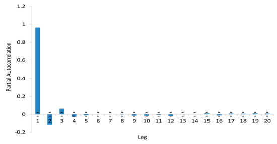
Figure 7.
Partial autocorrelation function for deseasoned wind-energy data.
After an AR(4) model is estimated, the fixed component is used to further improve the autoregressive model, and the general function of the modified CARDS models can be written as,
Here, Equation (8) indicates that for modified CARDS, we only need the AR model to capture the linear component and then use the fixed component to further improve the forecasting accuracy by modifying the forecasting of the AR model.
Figure 8 shows how for seven days the CARDS model fits with Starfish Hill wind farm energy data.
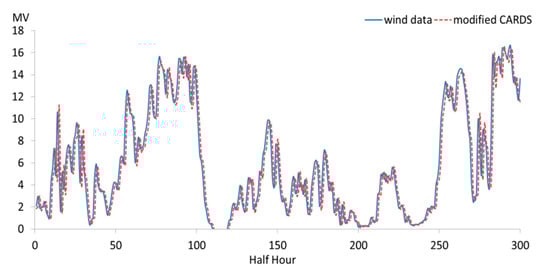
Figure 8.
Modified CARDS model compared with wind-energy data.
2.4. Hybrid Solar and Wind
Fourier series and CARDS models are still used here for forecasting hybrid solar and wind data. Again, we emphasize that the same model is used to maintain predictability analysis under the same benchmark. Table 4 shows that although the seasonal characteristics of the hybrid solar and wind system are less than solar itself, it still shows a fairly strong seasonal feature, with over 47% variance explained. All significant values are indicated in bold. Unlike solar energy, hybrid solar and wind energy only has strong once- and twice-daily cycles.
Table 4.
Fourier series analysis for hybrid solar and wind.
When the seasonal component is subtracted, the deseasoned data is analyzed by using autocorrelation analysis. The partial autocorrelation function shows that the residual is following an AR(3) model (see Figure 9). Then, the Lucheroni model and fixed component are used to set up the CARDS model for hybrid solar and wind data. Figure 10 shows Fourier series plus CARDS model compared with hybrid solar and wind-energy data.
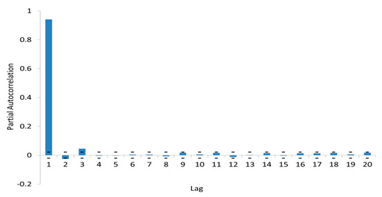
Figure 9.
Partial autocorrelation function for deseasoned hybrid data.
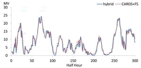
Figure 10.
CARDS model plus seasonal Fourier series compared with hybrid energy data.
3. Error Analysis
Error analysis is a very important step for data analysis and forecasting. It is a tool for finding which model is the best. Here, we use it to differentiate which type of data is easier to forecast. In Hoff et al.’s paper [33], error analyses are classified into two classes. One class consists of absolute dispersion errors which are root mean square error (RMSE) and mean absolute error (MAE). The other class represents relative percentage errors. Relative percentage errors use absolute dispersion error, such as RMSE or MAE, divided by the mean of the real data to produce a normalized value. Here, several of the most commonly used error value measures will be used. These are median absolute percentage error (MeAPE), mean bias error (MBE) and normalized root mean square error (NRMSE). MeAPE captures the size of the errors and avoids distorting the results for forecasting. If one uses mean absolute percentage error (MAPE), then with the variables under consideration, wind and solar, there are certain points in time that can produce large errors, and the distribution of errors becomes skewed. So, using MeAPE instead of MAPE for renewable-energy forecasting can provide a more accurate perspective. In turn, MBE is used to determine whether any particular model is more biased than another. NRMSE measures overall model quality related to the regression fit. What this means is how far the data deviates from the model, more specifically how far the regression line is from the line Y = X, where Y are the predicted values from the model, and X are the data values. These error functions are written as,
Here, is forecasting value, is measured value and is average of measured value.
Note that the whole forecasting series data (8784 (48 × 183) half-hourly wind and solar) is used for the error analysis here. Through the results of error analysis shown in Table 5, it can easily be seen that the forecasting of hybrid solar and wind is better than solar (the error analysis only includes a solar angle larger than 10 degrees) or wind on their own. From MBE, the hybrid solar and wind shows the overall error of the CARDS model plus Fourier series is almost zero. This indicates that the hybrid solar and wind method improves predictability compared to the component parts. The results of MeAPE explain that hybrid solar and wind are effectively reducing the median error of the data by 17.9% for solar data and 34.4% for wind data. For individual errors, the NRMSE shows that hybrid solar and wind can also improve the forecasting accuracy by 13.7% and 28% compared with solar and wind, respectively, if taken separately. From the above results, we can conclude that at least as far as the analyzed series are concerned, hybrid solar and wind can improve the accuracy of data prediction in the CARDS model and Fourier series. The result also confirms one of characteristics of the time-series analysis method which is that it is highly dependent on data from previous time steps. We believe that when solar and wind-energy data are added together, the relatively highly variable data at time t, time t – 1, and time t − 2 (AR(2) as an example) are transformed into relatively stabilized data series. Therefore, the hybrid solar and wind system shows a relatively small error. The reason for this is that the Lucheroni model combined with the AR and fixed component all contribute to reducing the effect of highly variable data in previous time steps.
Table 5.
Error analysis for solar, wind and hybrid solar and wind data; α is solar angle.
4. Conclusions
This paper analyzes the prediction accuracy of solar, wind and hybrid solar and wind data by using the CARDS model as the fundamental method. The paper begins by briefly introducing the recent research on hybrid solar and wind systems; the optimization of such systems is a hot topic for improving the stability of renewable-energy systems at the moment. Due to the variability of renewable energy supply, except for using different renewable-energy sources to complement each other, the authors further expound the benefits of using a hybrid renewable-energy system, more specifically wind and solar, from the perspective of predictability. The error analyses show that the errors are reduced by between 13% and 35% for both individual and whole data series error. This is also consistent with the features of the CARDS model based on the characteristics of time-series analysis methods which is that the value of forecasting is highly dependent on previous time-steps data. Therefore, we conclude that under the data series and the models used in this paper, the predictability of the hybrid system is higher than that of solar or wind systems considered individually. These results show a further advantage of the hybrid system over a single solar or wind system.
Author Contributions
Conceptualization, J.H. and J.B.; Methodology, J.H. and J.B.; Software, J.H. and J.B.; Validation, J.H. and J.B.; Formal Analysis, J.H.; Investigation, J.H.; Resources, J.H. and J.B.; Data Curation, J.H. and J.B.; Writing-Original Draft Preparation, J.H.; Writing-Review & Editing, J.H. and J.B.; Visualization, J.H.; Supervision, J.H.; Project Administration, J.H.; Funding Acquisition, J.H.
Acknowledgments
This work is supported by the Fundamental Research Funds for the Central Universities (grant No. 2015B12414).
Conflicts of Interest
The authors declare no conflict of interest.
Nomenclature
| CARDS | coupled autoregressive and dynamical system |
| AR | autoregressive |
| OSL | ordinary least squares |
| SETAR | self-exciting threshold autoregressive |
| STAR | smooth transition autoregressive |
| MeAPE | median absolute percentage error |
| MBE | mean bias error |
| NRMSE | normalized root mean square error |
References
- Lund, H.; Munster, E. Integrated energy systems and local energy markets. Energy Policy 2006, 34, 1152–1160. [Google Scholar] [CrossRef]
- Li, F. Market Reforms for Integrated Local Energy Systems. Proc. Chin. Soc. Electr. Eng. 2015, 35, 3693–3698. [Google Scholar]
- Von Wirth, T.; Gislason, L.; Seidl, R. Distributed energy systems on a neighborhood scale: Reviewing drivers of and barriers to social acceptance. Renew. Sustain. Energy Rev. 2018, 82, 2618–2628. [Google Scholar] [CrossRef]
- Blechinger, P.; Cader, C.; Bertheau, P.; Huyskens, H.; Seguin, R.; Breyer, C. Global analysis of the techno-economic potential of renewable energy hybrid systems on small islands. Energy Policy 2016, 98, 674–687. [Google Scholar] [CrossRef]
- Eltamaly, A.M.; Al-Shammaa, A.A. Optimal configuration for isolated hybrid renewable energy systems. J. Renew. Sustain. Energy 2016, 8, 045502. [Google Scholar] [CrossRef]
- Dagdougui, H.; Ouammi, A.; Sacile, R. A regional decision support system for onsite renewable hydrogen production from solar and wind energy sources. Int. J. Hydrog. Energy 2011, 36, 14324–14334. [Google Scholar] [CrossRef]
- Wolfgang, O.; Henden, A.L.; Belsnes, M.M.; Baumann, C.; Maaz, A.; Schaefer, A.; Moser, A.; Harasta, M.; Doble, T. Scheduling when reservoirs are batteries for wind- and solar-power. Energy Procedia 2016, 87, 173–180. [Google Scholar] [CrossRef][Green Version]
- Dali, M.; Belhadj, J.; Roboam, X. Hybrid solar–wind system with battery storage operating in grid-connected and standalone mode: Control and energy management—Experimental investigation. Energy 2010, 35, 2587–2595. [Google Scholar] [CrossRef]
- Kala, P.; Arora, S. A comprehensive study of classical and hybrid multilevel inverter topologies for renewable energy applications. Renew. Sustain. Energy Rev. 2017, 76, 905–931. [Google Scholar] [CrossRef]
- Michiorri, A.; Lugaro, J.; Siebert, N.; Girard, R.; Kariniotakis, G. Storage sizing for grid connected hybrid wind and storage power plants taking into account forecast errors autocorrelation. Renew. Energy 2018, 117, 380–392. [Google Scholar] [CrossRef]
- Orchi, T.F.; Mahmud, M.A.; Oo, A.M.T. Generalized Dynamical Modeling of Multiple Photovoltaic Units in a Grid-Connected System for Analyzing Dynamic Interactions. Energies 2018, 11, 296. [Google Scholar] [CrossRef]
- Sukumar, S.; Marsadek, M.; Ramasamy, A.; Mokhlis, H.; Mekhilef, S. A Fuzzy-Based PI Controller for Power Management of a Grid-Connected PV-SOFC Hybrid System. Energies 2017, 10, 1720. [Google Scholar] [CrossRef]
- Liu, L.; Wang, Z. The development and application practice of wind-solar energy hybrid generation systems in China. Renew. Sustain. Energy Rev. 2009, 13, 1504–1512. [Google Scholar] [CrossRef]
- Bekele, G.; Palm, B. Feasibility study for a standalone solar-wind-based hybrid energy system for application in Ethiopia. Appl. Energy 2010, 87, 487–495. [Google Scholar] [CrossRef]
- Zhou, W.; Lou, C.; Li, Z.; Lu, L.; Yang, H. Current status of research on optimum sizing of stand-alone hybrid solar-wind power generation systems. Appl. Energy 2010, 87, 380–389. [Google Scholar] [CrossRef]
- Liu, Y.; Yu, S.; Zhu, Y.; Wang, D.; Liu, J. Modeling, planning, application and management of energy systems for isolated areas: A review. Renew. Sustain. Energy Rev. 2018, 82, 460–470. [Google Scholar] [CrossRef]
- Micangeli, A.; del Citto, R.; Kiva, I.N.; Santori, S.G.; Gambino, V.; Kiplagat, J.; Vigano, D.; Fioriti, D.; Poli, D. Energy Production Analysis and Optimization of Mini-Grid in Remote Areas: The Case Study of Habaswein, Kenya. Energies 2017, 10, 2041. [Google Scholar] [CrossRef]
- Lukasievicz, T.; Oliveira, R.; Torrico, C. A Control Approach and Supplementary Controllers for a Stand-Alone System with Predominance of Wind Generation. Energies 2018, 11, 411. [Google Scholar] [CrossRef]
- Vasilj, J.; Sarajcev, P.; Jakus, D. Estimating future balancing power requirements in wind-PV power system. Renew. Energy 2016, 99, 369–378. [Google Scholar] [CrossRef]
- Peng, C.; Zou, J.; Zhang, Z.; Han, L.; Liu, M. An Ultra-Short-Term Pre-Plan Power Curve based Smoothing Control Approach for Grid-connected Wind-Solar-Battery Hybrid Power System. IFAC Papersonline 2017, 50, 7711–7716. [Google Scholar] [CrossRef]
- Akram, U.; Khalid, M.; Shafiq, S. Optimal sizing of a wind/solar/battery hybrid grid-connected microgrid system. IET Renew. Power Gener. 2018, 12, 72–80. [Google Scholar] [CrossRef]
- Petrakopoulou, F.; Robinson, A.; Loizidou, M. Simulation and evaluation of a hybrid concentrating-solar and wind power plant for energy autonomy on islands. Renew. Energy 2016, 96, 863–871. [Google Scholar] [CrossRef]
- Murat, G. Integration of hybrid power (wind-photovoltaic-diesel-battery) and seawater reverse osmosis systems for small-scale desalination applications. Desalination 2018, 435, 210–220. [Google Scholar]
- Quan, D.M.; Ogliari, E.; Grimaccia, F.; Leva, S.; Mussetta, M. Hybrid model for hourly forecast of photovoltaic and wind power. In Proceedings of the 2013 IEEE International Conference on Fuzzy Systems (FUZZ), Hyderabad, India, 7–10 July 2013; pp. 1–10. [Google Scholar]
- Zhang, Q.; Lai, K.K.; Niu, D.; Wang, Q.; Zhang, X. A Fuzzy Group Forecasting Model Based on Least Squares Support Vector Machine (LS-SVM) for Short-Term Wind Power. Energies 2012, 5, 3329–3346. [Google Scholar] [CrossRef]
- Huang, J.; Korolkiewicz, M.; Agrawal, M.; Boland, J. Forecasting solar radiation on an hourly time scale using a Coupled AutoRegressive and Dynamical System (CARDS) model. Sol. Energy 2013, 87, 136–149. [Google Scholar] [CrossRef]
- Lazard. In Lazard’s Latest Annual Levelized Cost of Energy Analysis (LCOE 11.0). 2017. Available online: https://www.lazard.com/perspective/levelized-cost-of-energy-2017 (accessed on 12 January 2018).
- Lucheroni, C. Resonating models for the electric power market. Phys. Rev. E 2007, 76, 056116. [Google Scholar] [CrossRef] [PubMed]
- Boland, J.; Hollands, K. Time series analysis of climatic variables (vol 55, pg 377, 1995). Sol. Energy 1996, 56, 637. [Google Scholar]
- Boland, J. Time Series and Statistical Modelling of Solar Radiation, Recent Advances in Solar Radiation Modelling; Badescu, V., Ed.; Springer: Berlin, Germany, 2008; pp. 283–312. [Google Scholar]
- Huang, J. Forecasting wind and solar energy on short time scales. Bull. Aust. Math. Soc. 2014, 89, 173–174. [Google Scholar] [CrossRef]
- Pinson, P.; Christensen, L.E.A.; Madsen, H.; Sorensen, P.E.; Donovan, M.H.; Jensen, L.E. Regime-switching modelling of the fluctuations of offshore wind generation. J. Wind Eng. Ind. Aerodyn. 2008, 96, 2327–2347. [Google Scholar] [CrossRef]
- Hoff, T.E.; Perez, R.; Kleissl, J.; Renne, D.; Stein, J. Reporting of irradiance modeling relative prediction errors. Prog. Photovolt. 2013, 21, 1514–1519. [Google Scholar] [CrossRef]
© 2018 by the authors. Licensee MDPI, Basel, Switzerland. This article is an open access article distributed under the terms and conditions of the Creative Commons Attribution (CC BY) license (http://creativecommons.org/licenses/by/4.0/).