Short-Term Solar Irradiance Forecasts Using Sky Images and Radiative Transfer Model

Abstract

In this paper, we propose a novel forecast method which addresses the difficulty in short-term solar irradiance forecasting that arises due to rapidly evolving environmental factors over short time periods. This involves the forecasting of Global Horizontal Irradiance (GHI) that combines prediction sky images with a Radiative Transfer Model (RTM). The prediction images (up to 10 min ahead) are produced by a non-local optical flow method, which is used to calculate the cloud motion for each pixel, with consecutive sky images at 1 min intervals. The Direct Normal Irradiance (DNI) and the diffuse radiation intensity field under clear sky and overcast conditions obtained from the RTM are then mapped to the sky images. Through combining the cloud locations on the prediction image with the corresponding instance of image-based DNI and diffuse radiation intensity fields, the GHI can be quantitatively forecasted for time horizons of 1–10 min ahead. The solar forecasts are evaluated in terms of root mean square error (RMSE) and mean absolute error (MAE) in relation to in-situ measurements and compared to the performance of the persistence model. The results of our experiment show that GHI forecasts using the proposed method perform better than the persistence model.

1. Introduction

The use of solar power as a renewable energy source has grown substantially over the last few decades. However, the amount of solar irradiance that reaches the Earth’s surface can vary significantly over relatively short time periods, resulting in fluctuation and intermittence of power generation. Therefore, it is crucial that we develop new techniques to accurately produce short-term forecasts of solar irradiance at the surface.

Historically, solar irradiance forecasts have relied heavily upon information retrieved via satellites and from Numerical Weather Prediction (NWP) models. Currently, NWP models generate forecasts in the range of 6 h to several days ahead [1,2] while satellite-based methods are generally used for 1 to 6-h period forecasts [3,4]. However, both NWP and satellite imagery lack the spatial and temporal resolutions necessary for providing detailed information regarding high frequency fluctuations of solar irradiance. To overcome this issue, ground-based sky imagers have been developed and deployed as a means of capturing local sky images with highly-refined spatial and temporal resolutions for intra-hour solar irradiance forecasts [5].

Cloudiness is the most significant determinant of the amount of solar radiation reaching the Earth’s surface [6]. The use of sky imagers allows us to accurately identify local cloud cover and subsequently, predict relative atmospheric evolution through the analysis of time series images. This information can be used to forecast changes in solar availability within time frames of 10–15 min for most environments. There are currently two main methods employed when utilizing sky-imagers for solar irradiance forecasting: Global Horizontal Irradiance (GHI) or Direct Normal Irradiance (DNI) which is directly obtained from the empirical relationship with cloud cover [7], and forecast models that integrate cloud images with machine learning techniques. Chow et al. [8] used digitally-processed sky images from Total Sky Imager (TSI) to detect cloud cover. The cloud images, which were used to calculate motion vectors by a cross-correlation method, were propagated forward in time resulting in an intra-hour forecast of GHI. Marquez and Coimbra [9] also made use of TSI for intra-hour DNI forecast, rather than GHI. This work computed the cloud field with Particle Image Velocimetry (PIV), which uses the minimum quadratic difference method to calculate velocity vectors for each segment from successive pairs of sky images. Then, they employed grid cloud fractions in an area of interest to forecast DNI. Bone et al. [10] used a clear-sky DNI model and a cloud fraction prediction algorithm to generate DNI predictions. The clear-sky model parameters were adaptively estimated from identified clear-sky DNI measurements over a moving window. The sector-ladder method, proposed by Quesada-Ruiz et al. [11], that computes 1-D radial cloud velocity vectors on a polar grid was modified to detect ramp events in the DNI predictions. Some researchers believe that it is necessary to use non-linear characteristics of machine learning methods to predict stochastic processes of solar radiation fluctuations. The machine learning methods for solar radiation forecast are various, such as Artificial Neural Network (ANN) [12,13], Support Vector Machine (SVM) [14,15], and k-Nearest Neighbor (k-NN) [16,17]. In the work of Chu et al. [13], the expected cloud cover indices were calculated using the method described by Marquez and Coimbra [9]. GHI forecasts that were 5, 10, and 15-min ahead of time were produced by ANNs that used the cloud indices and GHI lagged data as inputs. Cheng et al. [15] incorporated history measured irradiance data with features extracted from the all-sky images to perform predictions. The bi-model forecasting, which is trained according to cloud obstruction conditions near the solar disk, was constructed by support vector regressions. Pedro et al. [17] proposed a distribution-free methodology based on the k-Nearest-Neighbors (kNN) algorithm to predict intra-hour GHI and DNI irradiances using ground telemetry and sky images. Although forecast models based on machine learning methods achieve a lower rate of forecast errors, they can only predict GHI or DNI for specific time horizons, rather than producing a continuous solar irradiance forecast.

During broken cloud conditions, when the direct component of solar radiation is nearly unaffected, GHI at ground level often exceeds expected clear-sky values due to the scattering of the cloud in the sky. Additionally, when the sun is occluded, diffuse solar irradiance is the main energy component reaching the surface. Therefore, more accurate retrievals of the direct and diffuse components of solar irradiance will largely benefit GHI forecasts. The main novelty of this study is that Direct Normal Irradiance (DNI) and Diffuse Horizontal Irradiance (DHI) are quantitatively forecast within a 10-min time horizon by mapping the DNI value and downward diffuse radiation intensity fields obtained from Radiative Transfer Model (RTM) into the prediction sky images. The DNI model value and downward diffuse radiation intensity fields under clear sky and overcast conditions are calculated using the modified DISORT Radiative Transfer Model [18]. The corresponding prediction sky images are produced by the optical flow method described in Section 3.2.

The data used for solar irradiance forecast is presented in Section 2. Detailed methods are presented in Section 3, including sky image processing to detect cloud, cloud-motion field calculation via the optical flow method, solar irradiance simulation based on the modified DISORT RTM, and solar irradiance forecast through the use of prediction images in combination with corresponding DNI model values and the downward diffuse radiation intensity field. The results and discussion are presented in Section 4, and the conclusions are presented in Section 5.

2. Data

The Total Sky Imager (TSI) and Multifilter Rotating Shadowband Radiometer (MFRSR) are located at the Southern Great Plains (SGP) atmospheric observatory in Oklahoma, United States, which was the first field measurement site established by the Atmospheric Radiation Measurement (ARM) Climate Research Facility.

The TSI is located at 36.6060° N, 97.4850° W at an altitude of 316 m and is composed of a heated rotating hemispherical mirror with a down-pointing Charge Coupled Device (CCD) camera located above it. The mirror contains a sun tracking shadowband that continuously shields the mirror from direct sunlight in order to protect the camera sensor from the sun’s reflection [9]. Experimental Images of TSI are taken at 1 min intervals [19].

The MFRSR is a seven-channel radiometer with six passbands 10 nm Full Width Half Maxinum (FWHM) centered near 415, 500, 610, 665, 862, and 940 nm, and it contains an unfiltered silicon pyranometer [20]. It is positioned several hundred meters from the TSI with coordinates of 36.6050° N, 97.4850° W at an altitude of 318 m. It uses an automated shadowbanding technique to measure the total-horizontal, diffuse-horizontal, and direct-normal spectral irradiances through a single optical path [21]. In this study, the MFRSR channel at 415 nm, where gaseous absorption is minimal, was selected for solar irradiance forecasting. The sampling time of the DNI coincided with that of the TSI images. We used one-minute averages of DHI obtained from our three-sampling data, each of which was acquired at a 20s interval, as a means of eliminating any abnormal values caused by the cloud edge effect [19].

3. Method

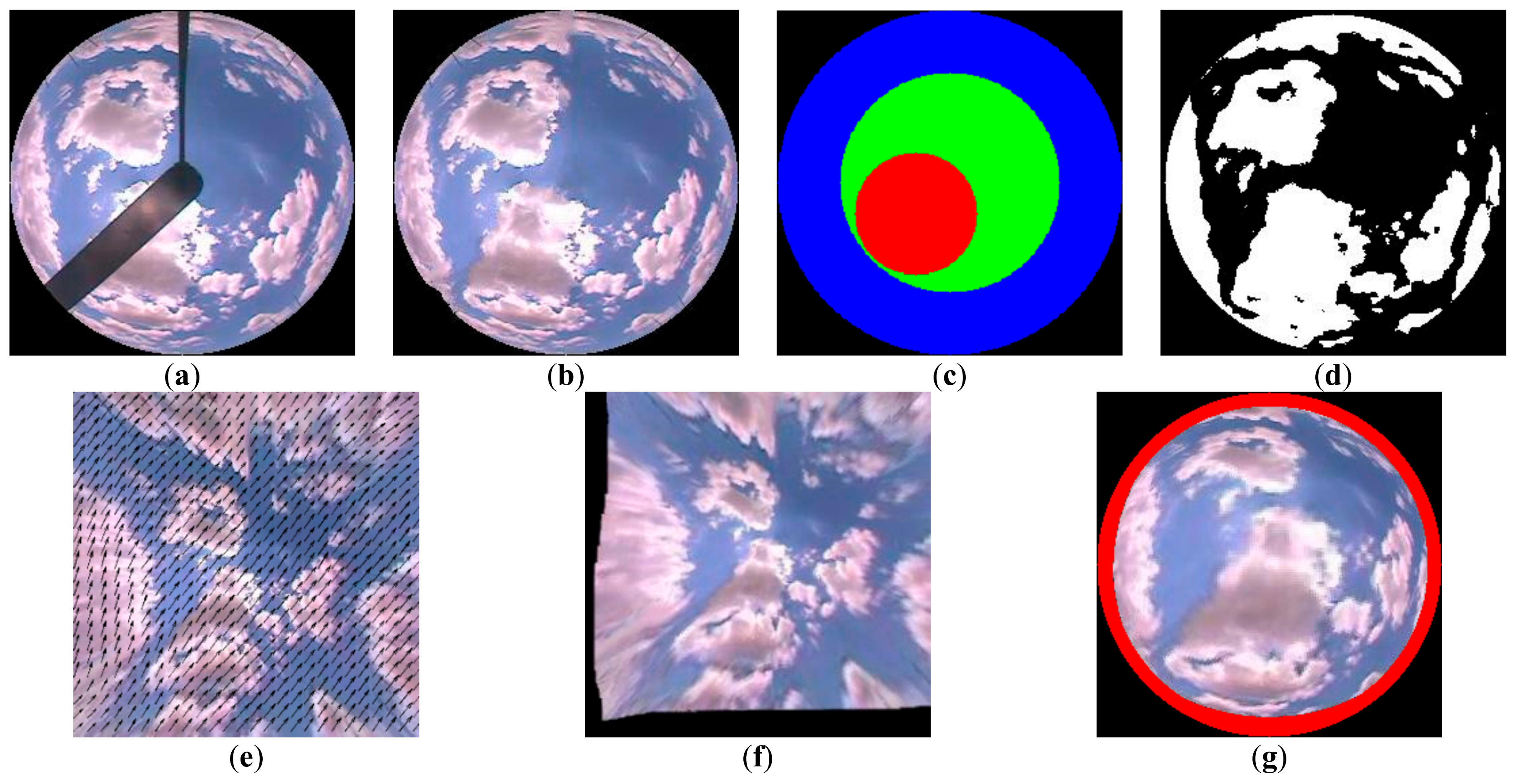
3.1. TSI Image Processing

Considering that pairs of consecutive TSI images are processed by an optical flow method to compute a cloud motion field, the shadowband areas of TSI images are filled by interpolation, as shown in Figure 1b.

A cloud detection method is then used to identify cloudy regions within the TSI images. Each pixel of the image is transferred into the normalized red to blue ratio, as defined by Yang et al. [22]:

$$\lambda =\frac{b-r}{b+r},$$

(1)

where b and r refer to the values of blue and red channels, respectively. The entire image of $\lambda$ intensities is partitioned into three regions in order to identify clouds, as illustrated in Figure 1c. The first region (red) is represented by the circular area with a radius of 45 pixels and is centered within the circumsolar position. The second region (green) is represented by the circle area of radius 80 pixels, but not including pixels in the first region. The third region (blue) includes any pixels not covered by the first and second regions. Each local threshold value, which segments the clear and cloudy part of the sky, is computed in the individual partitioned region using Ostu’s method [23]. The selected threshold value within the first region will be determined by whether or not the sun is occluded. Therefore, circularity is adopted to determine the sun’s occlusion [24]. The circularity is calculated for the circumsolar saturated pixels whose brightness is greater than 245 in the unsigned 8-bit image, using the following Equation (2) [25]:

$$C=4\cdot \mathsf{\pi }\cdot S/L^2,$$

(2)

where C is circularity, S refers to the area and L represents the perimeter. Higher values of C imply that the possibility of the sun being occluded is low. When the sun is not blocked by clouds (C ≥ 0.3), the threshold value is less than 0.05 to reduce any adverse effects on cloud detection caused by higher scattering of the direct beam. While the sun is occluded (C < 0.3), the threshold value is greater than 0.08 to better identify various types of cloud. The cloud detection image is shown in Figure 1d.

Lastly, all TSI images and cloud images are projected to a flat rectangular space for the purpose of removing the image distortion caused by the convex mirror. The steps are explained in detail by Marquez and Coimbra [9]. The pixel locations of the original image are converted into polar coordinates:

$$x_I=r_{I}cos\varphi ,$$

(3)

$$y_I=r_{I}sin\varphi ,$$

(4)

where $r_I$ is the radial distance from the zenith pole (center of image) to the pixels’ coordinate ($x_I,y_I$), and $\varphi$ is the azimuth angle with respect to the horizontal axis and refers to the image, $I$. Due to the image distortion, the relationship between $r_I$ and the tangent of the zenith angle ($\theta$) is nonlinear. The relationship between $r_I$ and $\theta$ is approximated by fitting pairs of the sun’s apparent radial distance ($r_{I,sun}$) and the corresponding solar zenith angle (${\theta }_s$) to obtain a cubic polynomial. The polynomial coefficients, $a_n$, are obtained using the Least Square Method for data computed from images of three selected clear sky days:

$$a_n=\left\{-0.0540,0.0140,0.8100,-0.0106\right\}.$$

An example of the projected image is shown in Figure 1e.

3.2. Computing Velocity Fields by the Optical Flow Method

The core idea of optical flow is to obtain the motion field between two successive frames of an image sequence while enforcing the following gradient constraint equation under the assumption of brightness constancy:

$$0=u\cdot I_x+v\cdot I_y+I_t,$$

(5)

where $I$ represents the pixel values in color or gray scale; $I_x,I_y$ and $I_t$ are the spatial and temporal partial derivatives of $I$ at time $t$; and $u$ and $v$ denote the velocity magnitude of each pixel’s motion vector in the $x$ and $y$ directions, respectively. The equation is an ill-posed problem because one equation with two unknowns, $u$ and $v$, cannot be solved without additional constraints. In order to solve this problem, Horn and Schunck [26] (abbreviated to HS) introduced the global strategy into the optical flow objective function. They formulated the optical flow as an optimization problem by minimizing the objective function under the assumption of brightness constancy and global smoothness of motions. Black and Anandan [27] (abbreviated to BA) introduced a non-convex robust penalty function into the objective of optical flow. They formulated the data term and the regularization term for smoothness with a series of non-quadratic robust penalty functions.

In this research, the optical flow method proposed by Sun et al. [28] was used to compute the motion field of sky images. They formulated a new weighted non-local term, which is added to the classical objective function descended from HS and BA, to prevent over-smoothing across boundaries. The formula by Sun et al. [28] is composed of four terms: the data term, the regularization term for smoothness, the coupling term and the weighted non-local term. Its spatially discrete form is as follows:

$$\begin{array}{cc}\hfill E_O\left(u,v,\widehat{u},\widehat{v}\right)=& {\displaystyle {\displaystyle \sum }_{i,j}}\{{\rho }_D\left(I_1\left(i,j\right)-I_2\left(i+u_{i,j},j+v_{i,j}\right)\right)\hfill \\ & +\lambda [{\rho }_s\left(u_{i,j}-u_{i+1,j}\right)+{\rho }_s\left(u_{i,j}-u_{i,j+1}\right)+{\rho }_s\left(v_{i,j}-v_{i+1,j}\right)\hfill \\ & +{\rho }_s\left(\left(v_{i,j}-v_{i,j+1}\right)\right)\left]\right\}+{\lambda }_c\left({\left|\left|u-\widehat{u}\right|\right|}^2+{\left|\left|v-\widehat{v}\right|\right|}^2\right)\hfill \\ & +{\displaystyle {\displaystyle \sum }_{i,j}}{\displaystyle {\displaystyle \sum }_{\left(i^{\prime },j^{\prime }\right)\in {\mathcal{N}}_{i,j}}}{\mathcal{W}}_{i,j}^{i^{\prime },j^{\prime }}\left(\left|{\widehat{u}}_{i,j}-{\widehat{u}}_{i^{\prime },j^{\prime }}\right|-\left|{\widehat{v}}_{i,j}-{\widehat{v}}_{i^{\prime },j^{\prime }}\right|\right),\hfill \end{array}$$

(6)

where $u$ and $v$ are the horizontal and vertical components of the optical flow field to be estimated from images $I_1$ and $I_2$; $\widehat{u}$ and $\widehat{v}$ denote an auxiliary flow field; $i,j$ indexes a particular image pixel location; $u_{i,j}$ and $v_{i,j}$ are elements of $u$ and $v,$ respectively; $\lambda$ is a regularization parameter; ${\lambda }_c$ is a scalar weight; ${\rho }_D$ and ${\rho }_s$ are the data and spatial penalty functions; ${\mathcal{N}}_{i,j}$ is the neighboring set of pixel ($i,j$) in a possible large area; and ${\mathcal{W}}_{i,j}^{i^{\prime },j^{\prime }}$ represents the likelihood of $i^{\prime },j^{\prime }$ belonging to the same surface as $i,j$. The weighting is defined by the spatial distance, color-value distance, and the occlusion state as

$${\mathcal{W}}_{i,j}^{i^{\prime },j^{\prime }}\propto \exp \left\{-\frac{{\left|i-i^{\prime }\right|}^2+{\left|j-j^{\prime }\right|}^2}{2{\sigma }_1^2}-\frac{{\left|I\left(i,j\right)-I\left(i^{\prime },j^{\prime }\right)\right|}^2}{2{\sigma }_2^2{n}_c}\right\}\frac{O\left(i^{\prime },j^{\prime }\right)}{O\left(i,j\right)},$$

(7)

where $I\left(i,j\right)$ is the color vector in the lab space that mathematically describes all perceivable colors in the three dimensions (L for lightness and a and b for the color components green-red and blue-yellow); $n_c$ is the number of color channels; and the occlusion variable, $O\left(i,j\right),$ is calculated as

$$O\left(i,j\right)=\exp \left\{-\frac{d^2\left(i,j\right)}{2{\sigma }_d^2}-\frac{{\left(I\left(i,j\right)-I\left(i+u_{i,j},j+v_{i,j}\right)\right)}^2}{2{\sigma }_e^2}\right\},$$

(8)

where $d\left(i,j\right)$ is the piecewise divergence function defined as

$$d\left(i,j\right)=\{\begin{array}{cc}\mathrm{div}\left(i,j\right),\hfill & \hfill \mathrm{div}\left(i,j\right)<0\\ 0,\hfill & \hfill otherwise\end{array},$$

(9)

in which the flow divergence, $\mathrm{div}\left(i,j\right),$ is

$$\mathrm{div}\left(i,j\right)=\frac{\partial }{\partial x}u\left(i,j\right)+\frac{\partial }{\partial y}v\left(i,j\right),$$

(10)

where $\frac{\partial }{\partial x}$ and $\frac{\partial }{\partial y}$ are, respectively, the horizontal and vertical flow derivatives. In practice, the weighting defined by Equation (7) in a $15\times 15$ neighborhood is used for the boundary regions, while equal weights in a $5\times 5$ neighborhood are used to compute the median in the non-boundary regions. The parameter setting is the same as that used by Sun et al. [28], consisting of $=3,{\lambda }_c=0.1$, ${\sigma }_1=7,{\sigma }_2=7,{\sigma }_d=0.3,{\sigma }_e=20$.

In addition to this method, several best practices were also used including a standard, incremental, multi-resolution technique to estimate flow fields with large displacements. In addition, the Rudin–Osher–Fatemi (ROF) structure texture decomposition method was used to preprocess the input image sequence to reduce the influence of lighting changes. Other methods included incremental warping and warping with the spline-based bicubic interpolation to obtain the lowest energy solutions, median filtering of intermediate flow results after each incremental estimation step to remove outliers, and a graduated non-convexity (GNC) scheme to minimize non-convex energies. In practice, a two-stage GNC scheme was used, with the penalty functions for the first and second stages being the quadratic penalty ($\rho \left(x\right)=x^2$), and the generalized Charbonnier penalty function ($\rho \left(x\right)={\left(x^2+{ϵ}^2\right)}^a,\epsilon =0.001,a=0.45$), respectively. The output of a previous stage served as the initialization to the next stage. An example of a velocity field calculation is shown in Figure 1e.

3.3. Solar Irradiance Simulation with RTM

In order to quantitatively predict GHI by calculating the direct and diffuse components of solar irradiance, it is necessary to estimate the cloud optical depth in the scene. We used the RTM to compute the DHI at different cloud optical depths and compared them with retrieved values from the nearby MFRSR, thereby allowing for the appropriate cloud optical depth to be chosen for GHI prediction.

3.3.1. Computing the Zenith and Azimuth Angle of Each Pixel on the Sky Image

The cartesian coordinates with respect to the central position of the image were $X=x-x_0,Y=y_0-y$, where $x_0,y_0$ are center coordinates of the image, and $x,y$ are the pixel coordinates on the image measured from the upper-left corner for columns and rows. The radial distance measured in pixels from the center position within the image is defined as $r=\sqrt{X^2+Y^2}$. We assumed that the center of the image was the zenith pole. Referring to the method for determining the relationship between the radial distance ($r$) and the zenith angle ($\theta$) of each pixel in Section 3.1, the zenith angle of each pixel can be computed from a fit cubic polynomial with the variable $r$:

$$\theta =0.3142r^3-0.2480r^2+1.3210r^2+0.002813.$$

(11)

The azimuth angle of each pixel ($\varphi$), which is the clockwise angle starting at zero on the left hand side, can be calculated by:

$$\varphi =\{\begin{array}{cc}{\cos }^{-1}\left(\frac{Y}{r}\right),\hfill & \hfill \mathrm{where}X\ge 0\\ 2\pi -{\cos }^{-1}\left(\frac{Y}{r}\right),\hfill & \hfill \mathrm{where}X<0\end{array}.$$

(12)

3.3.2. Locating the Sun’s Position on the Image

The solar position can be calculated for a specific location on Earth given the date and time. Using the algorithm provided by Reda and Andreas [29], the zenith angle (${\theta }_s$) and azimuth angle (${\varphi }_s$) of sun at time instance $i$ can be obtained. Then the coordinates of sun position ($x_s,y_s$) on the image are determined by:

$$x_s=x_0+r_{s}sin{\varphi }_s,$$

(13)

$$y_s=y_0-r_{s}cos{\varphi }_s,$$

(14)

where $r_s$ is the sun’s radial distance from the center position on the image, which can be calculated according to the relationship with the solar zenith angle, as described in Section 3.1.

3.3.3. Solar Irradiance Simulation with RTM

Using the modified DISORT Radiative Transfer Model, which combines the delta-fit method with the Nakajima–Tanaka correction procedure, we can accurately and rapidly compute radiances in both the forward and backward directions [18]. In addition, the direct and diffuse solar irradiances at the channel of nongaseous absorption wavelength (415 nm) can be simulated under various cloud optical depths with different solar zenith angles [30]. In the simulation, we used the Air Force Geophysics Laboratory (AFGL) midlatitude model, the aerosol profile from MODTRAN, 64 streams in the Legendre polynomial expansion, and surface albedos of 0.036 representing normal vegetated surfaces [21].

The RTM was initially utilized to establish a lookup table of the total optical thickness of Rayleigh scattering, gaseous absorption, and aerosol extinction at different solar zenith angles and visibilities. When clouds are broken and the sun is not occluded, the total optical thickness can be determined from direct beam measurements through the Bouguer–Lambert–Beer Law:

$$I_{dir}=\exp \left(-\tau A_0\right),$$

(15)

where $I_{dir}$ is the direct beam transmittance of the solar air mass ($A_0$), which is a function of the solar zenith angle; and $\tau$ is the total optical thickness of Rayleigh scattering, gaseous absorption, and aerosol extinction. The total optical thickness at different solar zenith angles calculated from MFRSR measurements is then compared with the lookup table to obtain the visibility at each time instance. The hourly average visibility is then derived from the calculated model parameter values of the direct and diffuse solar irradiances.

When the direct solar irradiance is calculated from the model values obtained by RTM, the pixel representing the position of the sun on the image and its four neighbourhoods are used to determine whether the sun is blocked. The direct solar irradiance is calculated by:

$$F_{dir}={\mathrm{DNI}}_{model}^{clr}\left(1-{\mathrm{CF}}_{sun}\right),$$

(16)

where $F_{dir}$ represents the computed direct irradiance; ${\mathrm{DNI}}_{model}^{clr}$ denotes the direct irradiance of RTM in the clear sky; and ${\mathrm{CF}}_{sun}$ is the cloud fraction calculated by the pixel representing the sun’s position and its four neighbourhoods. Figure 2 shows the calculated direct solar irradiance using the RTM on 7 July 2008. In Figure 2, the red solid line indicates the direct solar irradiance simulated by the RTM in the clear sky (clear sky DNI), the green dash line represents the direct solar irradiance computed by the RTM and the cloud image (Computed DNI), and the gray area is the measured value of the direct solar irradiance (measured DNI).

When the diffuse solar irradiance is computed, the simulated diffuse radiation intensity fields under clear sky and overcast conditions with different cloud optical depths are initially obtained from the RTM. In accordance with the zenith and azimuth angles of each pixel on the image calculated in Section 3.3.1, the diffuse radiation intensity fields can then be mapped to the image. The diffuse radiation intensity field under broken cloud conditions can be obtained by:

$$I=\{\begin{array}{c}{I}_{clr},\mathrm{where}\mathrm{pixel}=clearsky\hfill \\ I_{cld},\mathrm{where}\mathrm{pixel}=cloud\hfill \end{array},$$

(17)

where $I$, $I_{clr}$ and $I_{cld}$ represent the diffuse radiation intensity under broken clouds, clear sky and overcast conditions, respectively. The cloud image obtained from Section 3.1 is used to determine whether the pixel contains cloud or clear sky. Figure 3a–c show the image-based diffuse radiation intensity fields under clear sky, overcast and broken cloud conditions, respectively, at 19:37 (UTC) on 7 July 2008. Therefore, the total downward diffuse irradiance can be calculated by:

$$F_{dif}\left({\tau }_c\right)={{\displaystyle \int }}_0^{2\pi }d\varphi {{\displaystyle \int }}_0^1\mu I\left({\tau }_c,\mu ,\varphi \right)d\mu ,$$

(18)

where $F_{dif}\left({\tau }_c\right)$ denotes the total downward diffuse irradiance with different cloud optical depths and $\mu$ denotes the cosine of the zenith angle of the pixel. Figure 4 shows the total downward diffuse irradiance with different cloud optical depths on 7 July. In Figure 4, the black line indicates the measured value of the diffuse solar irradiance (measured DHI), the red solid line indicates the diffuse solar irradiance simulated by the RTM in the clear sky (clear sky DHI), the other solid lines of different colors indicate the diffuse solar irradiance simulated by the RTM under overcast conditions with different cloud optical depths (overcast DHI), and the short dash lines of different colors represent the diffuse solar irradiance computed from the cloud image and model value with different cloud optical depths (computed DHI).

In order to select the appropriate cloud optical depths for solar irradiance forecasts, the point sets consisting of the computed values of DHI for different cloud optical depths and the measured value of MFRSR were linearly fitted, respectively. The slope of the fitting line that is closest to 1 means that the difference between the computed value and the measured value is minimal.

3.4. Solar Irradiance Forecast

By using the optical flow method with two successive images at 1 min intervals, as described in Section 3.2, the prediction images and the cloud prediction images for time horizons of 1–10 min were initially obtained. Figure 1f,g show the prediction image in two coordinate systems. Figure 1f is the prediction image projected onto rectangular grid coordinates of the sky, and Figure 1g is the prediction image transformed from a rectangular grid to TSI image coordinates.

After that, the DNI and DHI were forecasted by the method described in Section 3.3 with the RTM and corresponding cloud prediction image. However, there are two scenarios that must be accounted for when using the cloud prediction image. One is that the solar irradiance cannot be forecast when the sun position on the image is not within the cloud prediction image. The other occurs when there is an area that cannot be covered by the prediction image, as shown in Figure 1g. The diffuse solar irradiance of this area is estimated by:

$$F_{DHI}^{uncover}=\mathrm{CF}\left(F_{model}^{cld}-F_{predict}^{cld}\right)+\left(1-\mathrm{CF}\right)\left(F_{model}^{clr}-F_{predict}^{clr}\right),$$

(19)

where $\mathrm{CF}$ represents the cloud fraction computed by the cloud prediction image; $F_{model}^{cld}$ and $F_{model}^{clr}$ denote the diffuse irradiance of RTM under overcast and clear sky conditions, respectively; $F_{predict}^{cld}$ and $F_{predict}^{clr}$ denote the diffuse irradiance in the range of the prediction image under overcast and clear sky conditions, respectively; and $F_{DHI}^{uncover}$ denotes the forecast diffuse irradiance of the uncovered area. Therefore, the forecast GHI is calculated by:

$$F_{GHI}=F_{DNI}^{predict}+F_{DHI}^{predict}+F_{DHI}^{uncover},$$

(20)

where $F_{GHI}$ is the forecast value of GHI, and $F_{DNI}^{predict}$ and $F_{DHI}^{predict}$ denote the forecast values of the direct and diffuse solar irradiances from the cloud prediction image, respectively.

4. Result and Discussion

The experimental dataset comprised daylight hours observed on 20–21 June, and 7 July 2008. These days all had broken cloud conditions with periods of clear sky. However, the cloud fraction throughout the days varied. The cloud cover was least on 20 June and gradually increased on 21 June. The greatest cloud cover occurred on 7 July. A limited number of partly cloudy days is more useful when evaluating short-term forecasts than a prolonged period of many clear sky days and overcast days. Error averages would likely be affected due to the fact that clear sky days and overcast days contain very little forecast error.

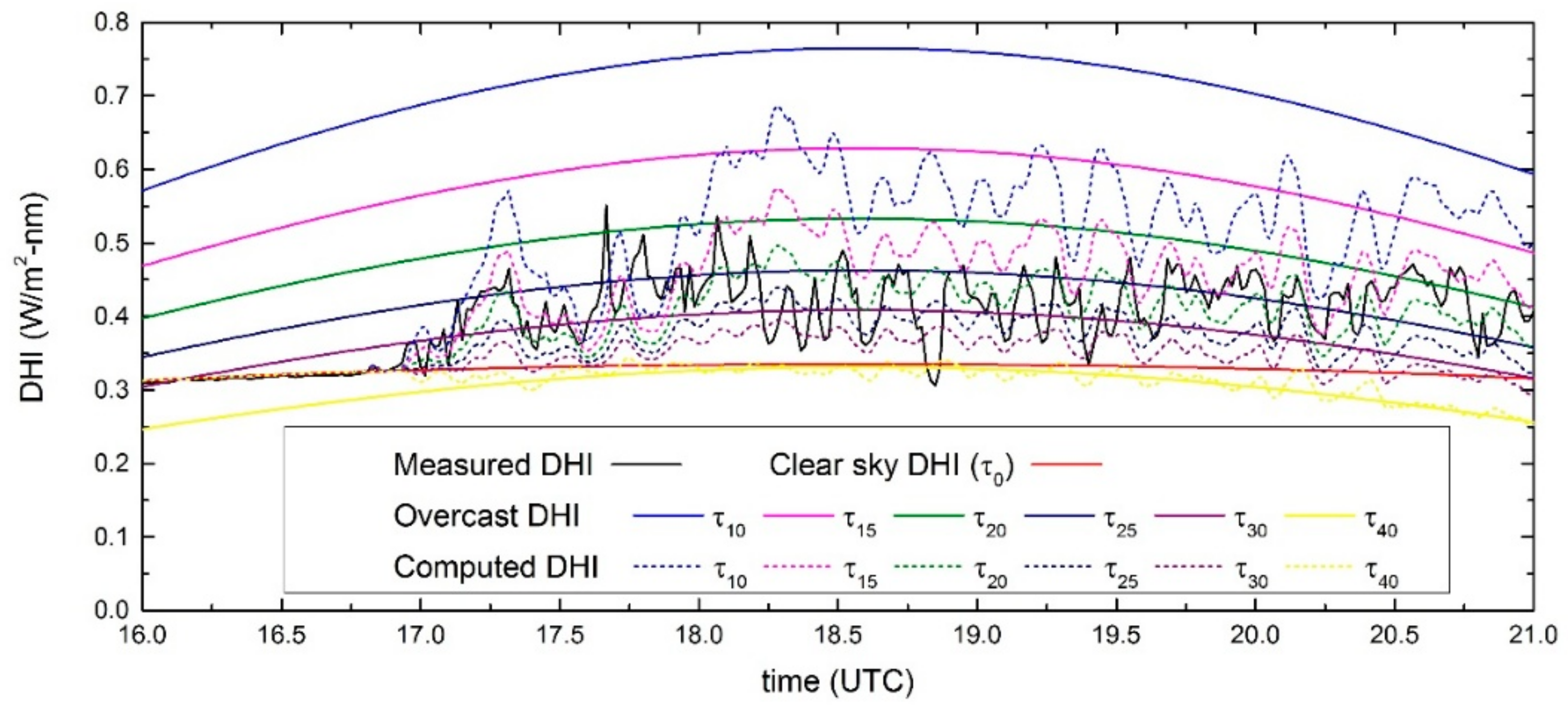
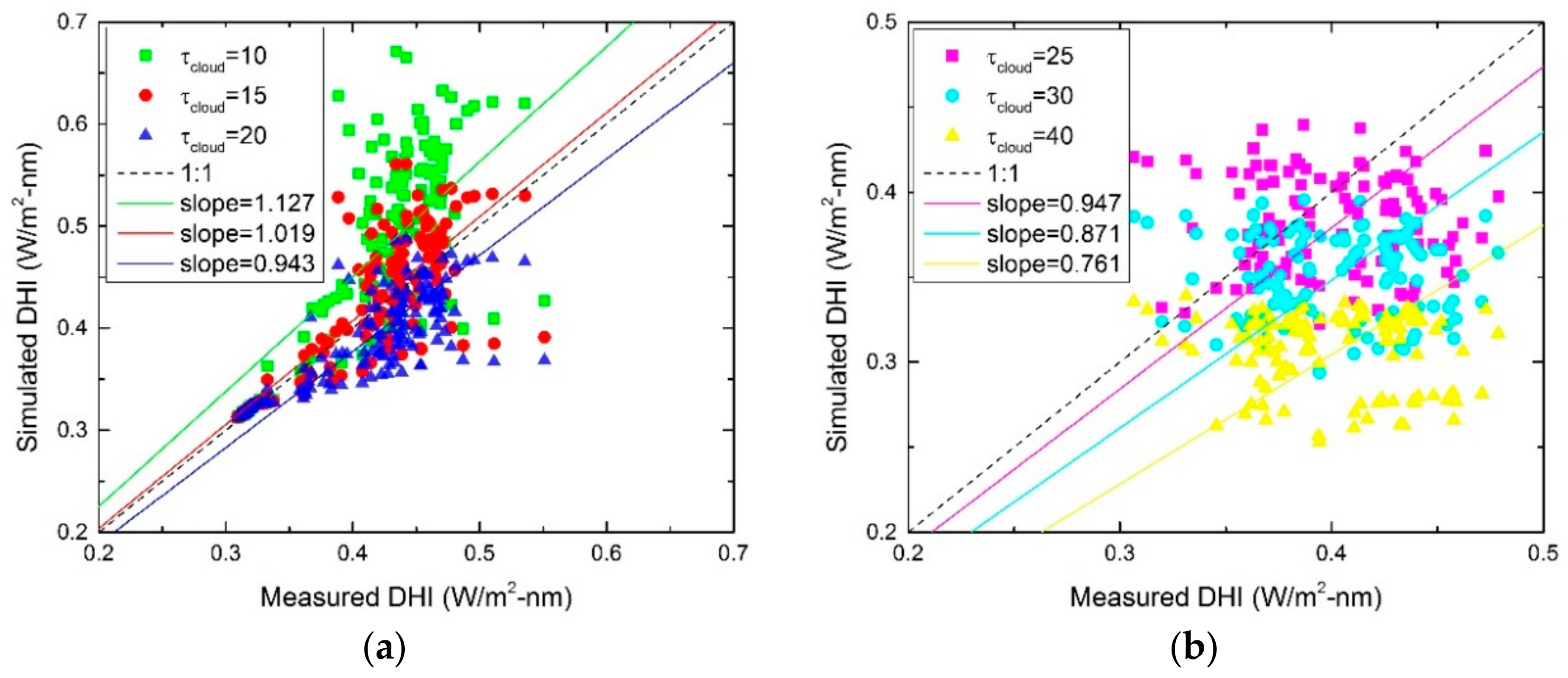
4.1. Selecting Appropriate Cloud Optical Depths

The diffuse solar irradiance computed with the RTM was divided into two parts, depending on whether or not the sun was occluded, and was then respectively compared to measured DHI values. Figure 5 shows the linear fitting results of scatter points consisting of the DHI computed with RTM and the DHI values measured on 7 July. The anomalous points of the measured value of DHI were caused by the cloud edge effect. When the sun was not blocked, the slope of the fitting line with cloud optical depth of 15 was closest to 1 (as seen in Figure 5a). When the sun was blocked, the slope of the fitting line with cloud optical depth of 25 was closest to 1 (as seen in Figure 5b). Therefore, these two cloud optical depths were used as cloud parameters for solar irradiance forecasting.

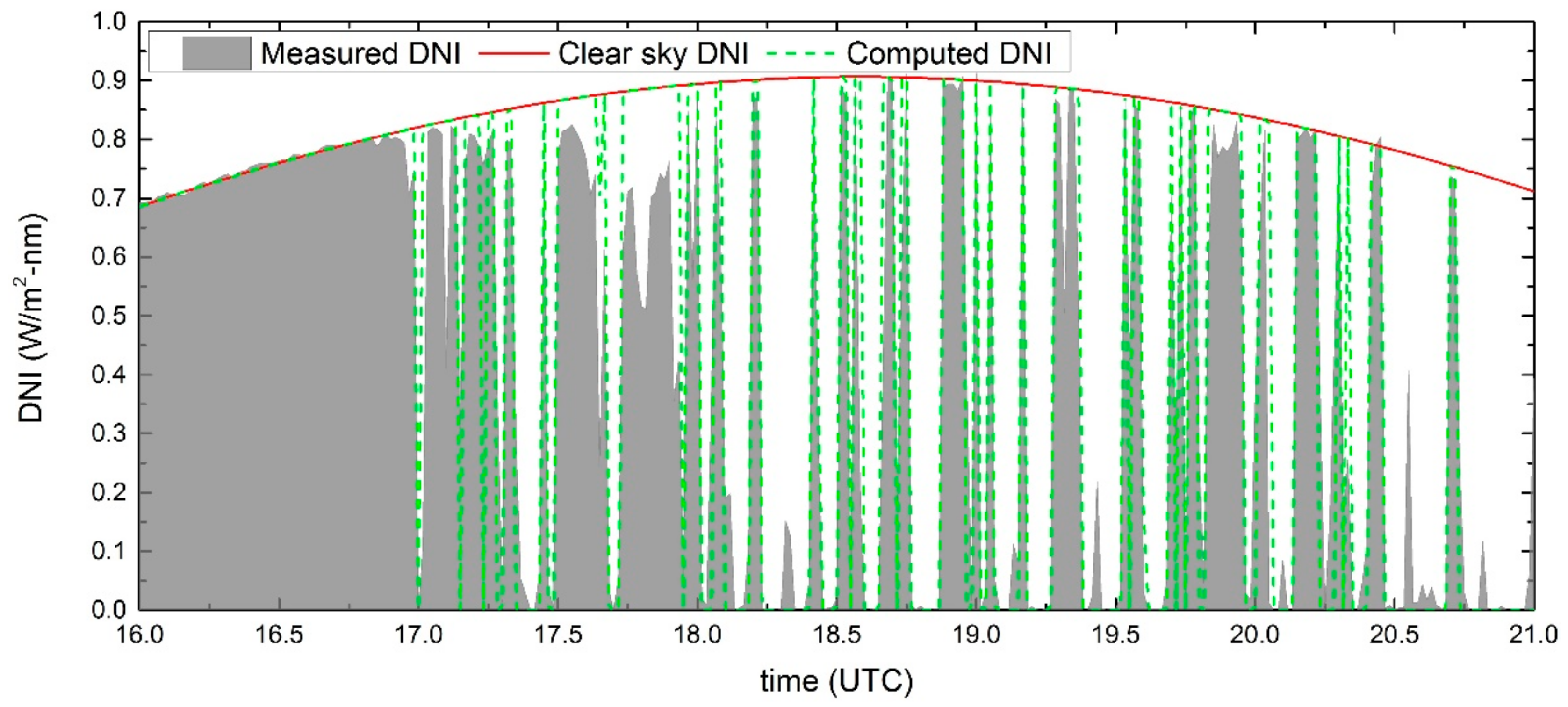
4.2. Evaluating the Error of Solar Irradiance Simulation with RTM

The metric used to evaluate the simulation error was the Mean Absolute Error (MAE), defined as:

$$\mathrm{MAE}=\frac{1}{n}{{\displaystyle \sum }}_t^n\left|\widehat{F}\left(t\right)-F\left(t\right)\right|,$$

(21)

where $F\left(t\right)$ denotes the measured irradiance at time instance $t$, $\widehat{F}\left(t\right)$ denotes the corresponding computed irradiance, and $n$ denotes the number of simulated samples.

Table 1. Mean Absolute Error (MAE) in W/m²-nm of the simulated Direct Normal Irradiance (DNI), Diffuse Horizontal Irradiance (DHI) and Global Horizontal Irradiance (GHI).

	DNI	DHI	GHI
20 June 2008	0.037	0.014	0.039
21 June 2008	0.043	0.033	0.064
7 July 2008	0.073	0.032	0.088

shows the MAE values of the DNI, DHI and GHI computed by the RTM over these three days. From Table 1, it can be seen that the MAE values of DNI, DHI and GHI all increased with increasing the cloud cover. The main reason for the DNI inconsistency is that the direct solar energy is transmitted through the clouds. The ground measurements in this condition were greater than zero. However, the value calculated by the RTM was zero in the above condition. Another reason for the larger error in DNI on 7 July is the existence of optically thinner clouds during the period from 17.5 to 18 h. The attenuation of direct solar irradiance by thinner clouds during this period resulted in measured DNI values being less than those measured under clear sky conditions (seen in Figure 3). This type of cloud is difficult to detect because it is blue-tinted. Therefore, the measured values are less than computed values under these conditions. There are two reasons for the error in DHI. First, the measured values are abnormally higher than the computed values due to the cloud edge effect. Moreover, the DHI values computed by the RTM are not identical to the measured values because of the change in cloud optical depths caused by the variance in cloud shape and size over time. In addition, the errors between the GHI data simulated by the sky images and the measured data are due to the fact that the TSI and the MFRSR are hundreds of meters apart. When the sun is at the edge of the cloud, there may be a situation where the cloud blocks the direct solar radiation to the MFRSR but not to the sky imager, or vice versa.

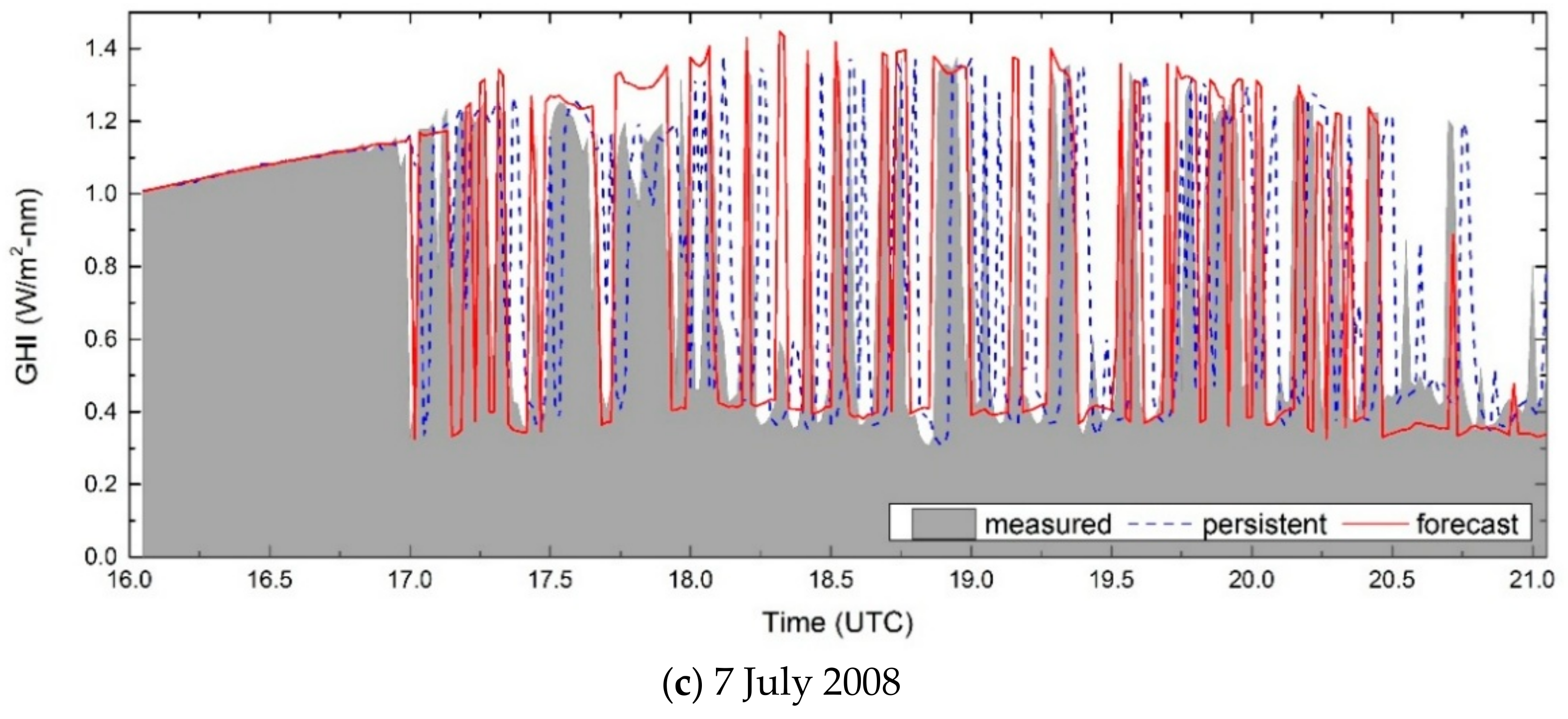
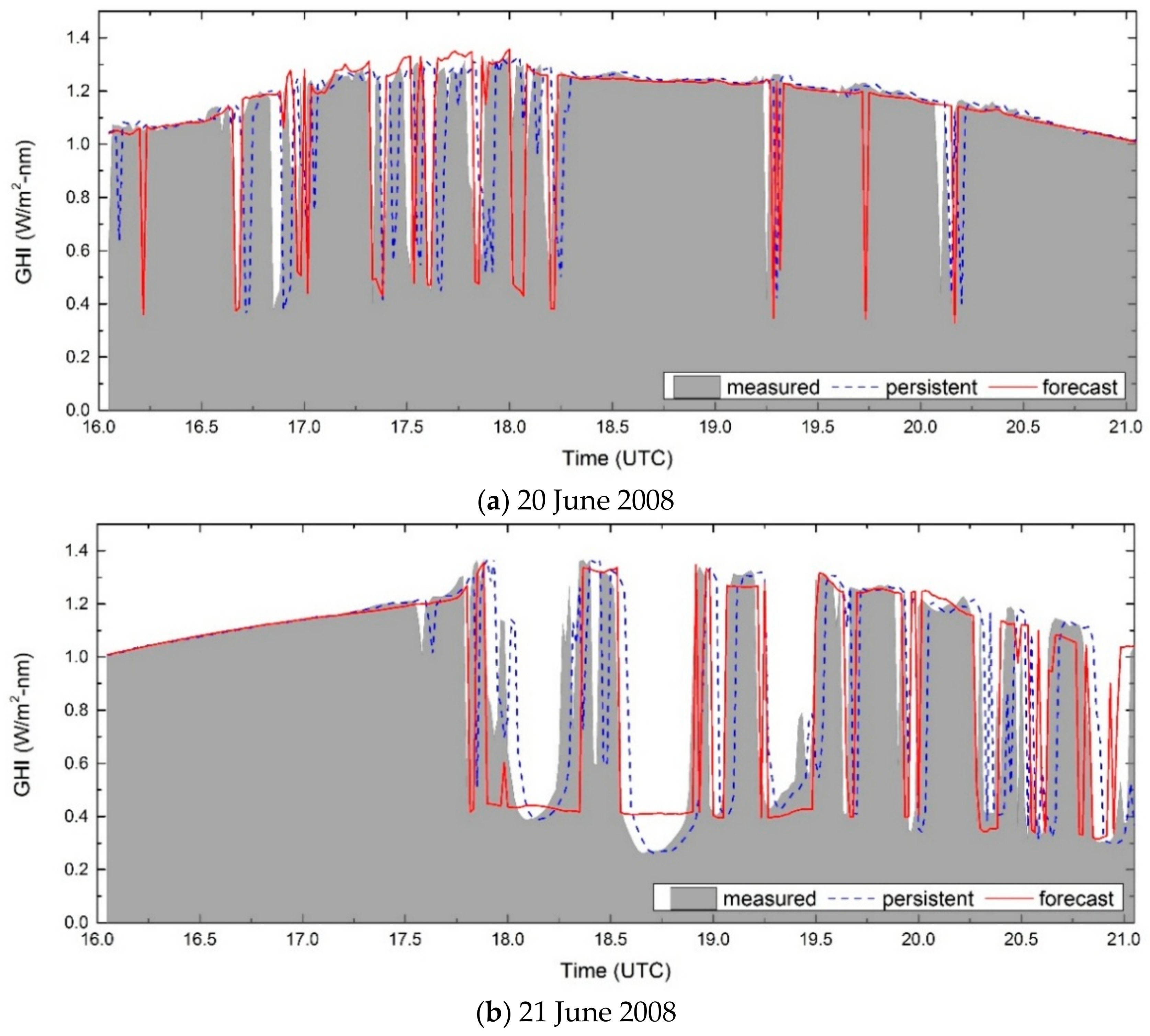
4.3. Solar Irradiance Forecast Performance

The persistence model is the simplest forecasting model and is often used as a baseline for the performance evaluation of other forecast models. Persistence forecasts are defined as only considering current deviations from clear sky conditions for subsequent forecast time horizons. The persistence forecast of the solar irradiance at the next time step is computed as [7]:

$$F_p\left(t+\mathsf{\Delta }t\right)=\frac{F\left(t\right)}{F_{clr}\left(t\right)}{F}_{clr}\left(t+\mathsf{\Delta }t\right),$$

(22)

where $\mathsf{\Delta }t$ is the forecast time horizon; $F\left(t\right)$ and $F_{clr}\left(t\right)$ denote the measured irradiance and the modelled clear sky irradiance at time instance $t$, respectively; $F_p\left(t+\mathsf{\Delta }t\right)$ represents the forecast value of the persistence model at each forecasting horizon; and $F_{clr}\left(t+\mathsf{\Delta }t\right)$ represents the modelled clear sky irradiance at the corresponding forecasting horizon.

The metrics used to evaluate the prediction error for each forecasting horizon were the Root Mean Square Error (RMSE) and MAE, as defined by:

$$\mathrm{RMSE}\left(\mathsf{\Delta }t\right)=\sqrt{\frac{1}{n}{{\displaystyle \sum }}_t^n{\left(\widehat{F}\left(t+\mathsf{\Delta }t\right)-F\left(t+\mathsf{\Delta }t\right)\right)}^2},$$

(23)

$$\mathrm{MAE}\left(\mathsf{\Delta }t\right)=\frac{1}{n}{{\displaystyle \sum }}_t^n\left|\widehat{F}\left(t+\mathsf{\Delta }t\right)-F\left(t+\mathsf{\Delta }t\right)\right|,$$

(24)

where $F\left(t+\mathsf{\Delta }t\right)$ denotes the measured irradiance at time instance ($t+\mathsf{\Delta }t$); $\widehat{F}\left(t+\mathsf{\Delta }t\right)$ denotes the corresponding forecast solar irradiance computed by the persistence model or proposed forecast model; and $n$ denotes the number of prediction samples.

Table 2. RMSE and MAE in W/m2-nm computed for forecasting horizons of 1–10 min.

Forecast Horizon	20 June 2008				21 June 2008				7 July 2008
	Presented Model		Persistence Model		Presented Model		Persistence Model		Presented Model		Persistence Model
	RMSE	MAE	RMSE	MAE	RMSE	MAE	RMSE	MAE	RMSE	MAE	RMSE	MAE
1	0.196	0.074	0.206	0.082	0.226	0.095	0.270	0.131	0.346	0.193	0.349	0.200
2	0.217	0.085	0.254	0.113	0.257	0.124	0.293	0.144	0.316	0.171	0.432	0.280
3	0.240	0.098	0.272	0.123	0.280	0.139	0.339	0.181	0.321	0.175	0.461	0.305
4	0.241	0.098	0.278	0.129	0.287	0.143	0.379	0.217	0.379	0.218	0.487	0.328
5	0.237	0.097	0.275	0.129	0.301	0.156	0.403	0.240	0.388	0.226	0.502	0.348
6	0.265	0.120	0.274	0.125	0.326	0.174	0.427	0.265	0.419	0.253	0.495	0.344
7	0.266	0.122	0.272	0.124	0.334	0.178	0.436	0.273	0.441	0.273	0.479	0.325
8	0.280	0.130	0.285	0.137	0.337	0.178	0.452	0.292	0.442	0.277	0.480	0.324
9	0.289	0.142	0.319	0.154	0.353	0.193	0.467	0.305	0.424	0.260	0.477	0.327
10	0.285	0.136	0.327	0.160	0.360	0.197	0.472	0.309	0.448	0.280	0.486	0.334

shows the RMSE and MAE of GHI calculated by Equations (23) and (24) for the proposed forecast model and the persistence model in the above three days. It is known that the persistence model produces accurate forecasts when the variability of solar irradiance is low. From Table 2, it can be seen that the persistence model errors on these three days showed an increasing trend, which indicates that the fluctuation of the solar irradiance is more frequent with an increase in cloud fraction. During these three days, the number of errors in the proposed forecast model for each forecast horizon were less than the number of errors in the persistence model, which means that the proposed forecast model improves the estimation over random variability. However, as the forecast horizon becomes longer, the errors are larger due to rapid cloud deformation, formation, or evaporation.

The GHI forecasting error can be evaluated further by making comparisons with the persistence model error. The forecast skill ($s$) is computed as:

$$s=1-\frac{{\mathrm{RMSE}}_f}{{\mathrm{RMSE}}_p},$$

(25)

where ${\mathrm{RMSE}}_f$ and ${\mathrm{RMSE}}_p$ represent the RMSE for the proposed forecast model and persistence model, respectively. Skill values greater than zero imply that the proposed forecast method outperforms the persistence model. Figure 6 shows forecast skill values for the entire evaluation period. In Figure 6, it can be seen that there were higher forecast skill values at forecast horizons of 2–5 min. During these periods, cloud deformation, formation, and evaporation are relatively small so the cloud prediction image could be used for a more accurate quantitative forecast of solar irradiance. The lower predictability of 1 min is due to the fact that the shadowband area of TSI is too wide to cause the loss of information around the sun. For example, when the cloud is in the shadowband area, this cloud may not be obtained for the interpolated image, which could lead to an incorrect cloud prediction image at the next forecasting time. Time-series plots of the measured values, persistence model, and 3-min forecasts with the highest forecast skill are shown in Figure 7. From these figures, it can be found that the forecasts showed considerable improvement in the persistence of predicting the effect of cloud transience on GHI, especially during the period where there was a high frequency of fluctuation. Meanwhile, we also found that when the sun was obstructed by the cloud, the GHI measured values changed with the cloud fraction and cloud optical depth. Therefore, compared to the method of giving a fixed GHI estimated value when the sun is predicted to be blocked, our proposed method can obtain more accurate prediction results through qualitatively calculating the GHI values with the use of the cloud prediction image and RTM.

5. Conclusions

This paper aimed to use the Radiative Transfer Model and its corresponding TSI prediction image to quantitatively forecast DNI and DHI for time horizons shorter than 10 min. The main processes were the following:

(1)

The prediction images were produced by image processing, which includes cloud detection, spatial transformation of TSI images, and cloud motion field calculation. The non-local optical flow method was able to capture the independent velocity vector of each pixel across successive images.

(2)

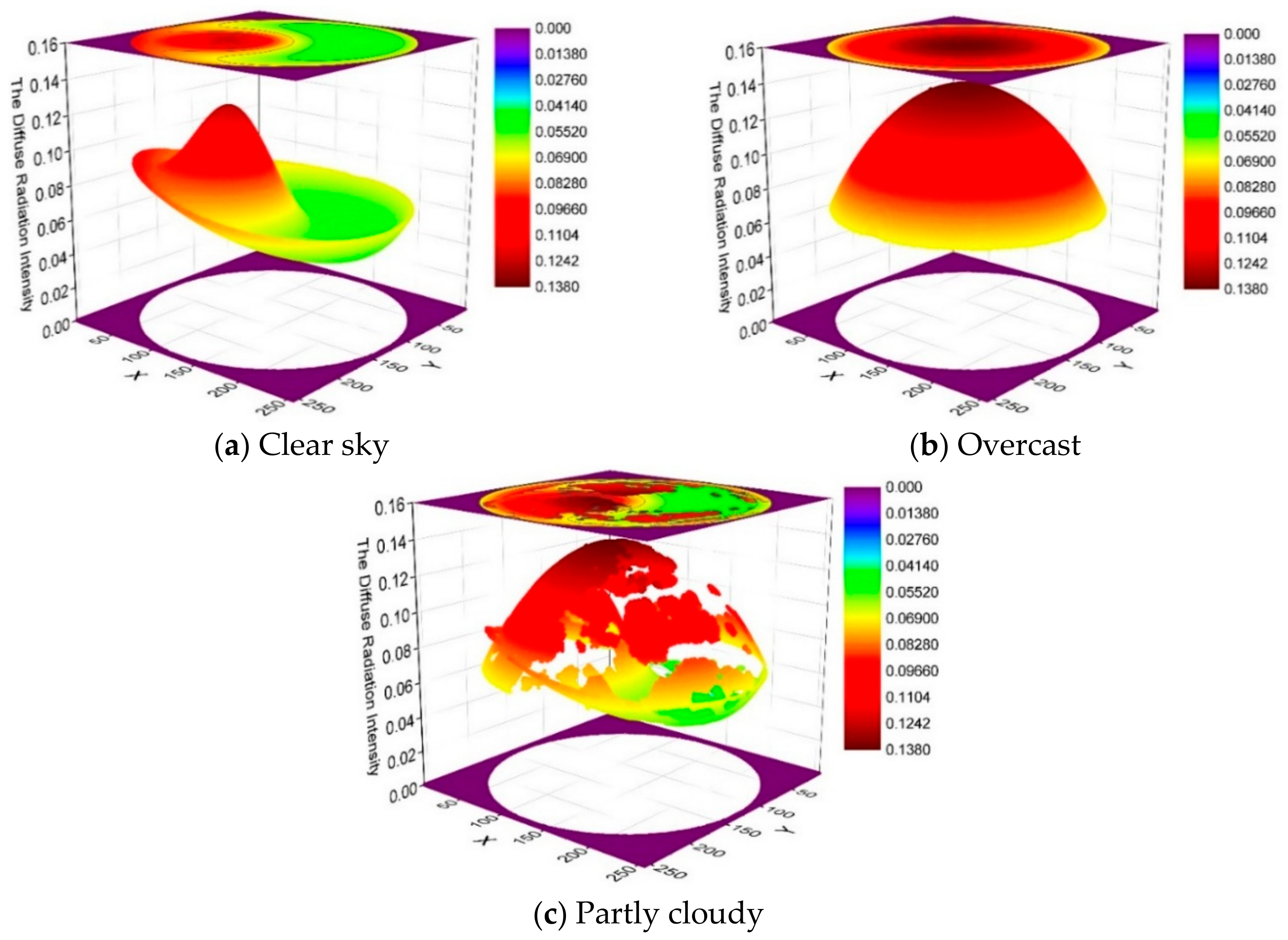
The direct and diffuse solar irradiances simulated by the RTM were compared with in-situ measurements to determine model parameters—visibility and cloud optical depth. One of the key steps was to produce the image-based diffuse radiation intensity field under broken cloud conditions.

(3)

The direct and diffuse solar irradiances were forecasted from DNI model values and the diffuse radiation intensity field with certain cloud optical depths obtained from the RTM and corresponding cloud prediction images.

Three partly cloudy days with different cloud cover fractions were chosen to demonstrate the methodology. The RMSE and MAE errors of the presented forecast model were less than those of the persistence model, validating the use of prediction images combined with the RTM for 1-10 min, short-term forecasting horizons.

At the same time, there are some limitations to the proposed method and the existing instruments: (1) the proposed method may generate large errors in the presence of optically thin cloud layers due to their blue-tinting effect; (2) all clouds in images containing the same optical depth values as in the RTM may cause a certain number of DHI errors; (3) the wide shadowband of TSI and the distance between TSI and MFRST could cause the prediction errors. However, all in all, these situations open new possibilities for optimizing the current method and designing a new instrument integrating the sky imager and ground-based radiometer in future work.

References

1. Perez, R.; Lorenz, E.; Pelland, S.; Beauharnois, M.; Van Knowe, G.; Hemker, K.; Heinemann, D.; Remund, J.; Muller, S.C.; Traunmuller, W.; et al. Comparison of numerical weather prediction solar irradiance forecasts in the US, Canada and Europe. Sol. Energy 2013, 94, 305–326. [Google Scholar] [CrossRef]
2. Lauret, P.; David, M.; Pedro, H.T.C. Probabilistic solar forecasting using quantile regression models. Energies 2017, 10, 1591. [Google Scholar] [CrossRef]
3. Kidd, C.; Levizzani, V.; Bauer, P. A review of satellite meteorology and climatology at the start of the twenty-first century. Prog. Phys. Geogr. 2009, 33, 474–489. [Google Scholar] [CrossRef]
4. Marquez, R.; Pedro, H.T.C.; Coimbra, C.F.M. Hybrid solar forecasting method uses satellite imaging and ground telemetry as inputs to ANNs. Sol. Energy 2013, 92, 176–188. [Google Scholar] [CrossRef]
5. Barbieri, F.; Rajakaruna, S.; Ghosh, A. Very short-term photovoltaic power forecasting with cloud modeling: A review. Renew. Sustain. Energy Rev. 2017, 75, 242–263. [Google Scholar] [CrossRef]
6. Matuszko, D. Influence of the extent and genera of cloud cover on solar radiation intensity. Int. J. Climatol. 2012, 32, 2403–2414. [Google Scholar] [CrossRef]
7. Inman, R.H.; Pedro, H.T.C.; Coimbra, C.F.M. Solar forecasting methods for renewable energy integration. Prog. Energy Combust. 2013, 39, 535–576. [Google Scholar] [CrossRef]
8. Chow, C.W.; Urquhart, B.; Lave, M.; Dominguez, A.; Kleissl, J.; Shields, J.; Washom, B. Intra-hour forecasting with a total sky imager at the UC San Diego solar energy testbed. Sol. Energy 2011, 85, 2881–2893. [Google Scholar] [CrossRef]
9. Marquez, R.; Coimbra, C.F.M. Intra-hour DNI forecasting based on cloud tracking image analysis. Sol. Energy 2013, 91, 327–336. [Google Scholar] [CrossRef]
10. Bone, V.; Pidgeon, J.; Kearney, M.; Veeraragavan, A. Intra-hour direct normal irradiance forecasting through adaptive clear-sky modelling and cloud tracking. Sol. Energy 2018, 159, 852–867. [Google Scholar] [CrossRef]
11. Quesada-Ruiz, S.; Chu, Y.; Tovar-Pescador, J.; Pedro, H.T.C.; Coimbra, C.F.M. Cloud-tracking methodology for intra-hour DNI forecasting. Sol. Energy 2014, 102, 267–275. [Google Scholar] [CrossRef]
12. Wang, F.; Mi, Z.Q.; Su, S.; Zhao, H.S. Short-term solar irradiance forecasting model based on artificial neural network using statistical feature parameters. Energies 2012, 5, 1355–1370. [Google Scholar] [CrossRef]
13. Chu, Y.H.; Pedro, H.T.C.; Nonnenmacher, L.; Inman, R.H.; Liao, Z.Y.; Coimbra, C.F.M. A smart image-based cloud detection system for intrahour solar irradiance forecasts. J. Atmos. Ocean. Technol. 2014, 31, 1995–2007. [Google Scholar] [CrossRef]
14. Long, H.; Zhang, Z.J.; Su, Y. Analysis of daily solar power prediction with data-driven approaches. Appl. Energy 2014, 126, 29–37. [Google Scholar] [CrossRef]
15. Cheng, H.Y.; Yu, C.C.; Lin, S.J. Bi-model short-term solar irradiance prediction using support vector regressors. Energy 2014, 70, 121–127. [Google Scholar] [CrossRef]
16. Wei, C.C. Predictions of surface solar radiation on tilted solar panels using machine learning models: A case study of Tainan city, Taiwan. Energies 2017, 10, 1660. [Google Scholar] [CrossRef]
17. Pedro, H.T.C.; Coimbra, C.F.M. Nearest-neighbor methodology for prediction of intra-hour global horizontal and direct normal irradiances. Renew. Energy 2015, 80, 770–782. [Google Scholar] [CrossRef]
18. Min, Q.L.; Joseph, E.; Duan, M.Z. Retrievals of thin cloud optical depth from a multifilter rotating shadowband radiometer. J. Geophys. Res. Atmos. 2004, 109, D02201. [Google Scholar] [CrossRef]
19. Data Sources. Available online: https://www.arm.gov/data/data-sources (accessed on 20 April 2018).
20. Harrison, L.; Michalsky, J.; Berndt, J. Automated multifilter rotating shadow-band radiometer—An instrument for optical depth and radiation measurements. Appl. Opt. 1994, 33, 5118–5125. [Google Scholar] [CrossRef] [PubMed]
21. Min, Q.L.; Wang, T.H.; Long, C.N.; Duan, M.Z. Estimating fractional sky cover from spectral measurements. J. Geophys. Res. Atmos. 2008, 113, D20208. [Google Scholar] [CrossRef]
22. Yang, J.; Lu, W.T.; Ma, Y.; Yao, W. An automated cirrus cloud detection method for a ground-based cloud image. J. Atmos. Ocean. Technol. 2012, 29, 527–537. [Google Scholar] [CrossRef]
23. Otsu, N. A threshold selection method from gray-level histograms. IEEE Trans. Syst. Man Cybern. 1979, 9, 62–66. [Google Scholar] [CrossRef]
24. Yang, J.; Min, Q.; Lu, W.; Yao, W.; Ma, Y.; Du, J.; Lu, T.; Liu, G. An automated cloud detection method based on the green channel of total-sky visible images. Atmos. Meas. Tech. 2015, 8, 4671–4679. [Google Scholar] [CrossRef]
25. Montero, R.S.; Bribiesca, E. State of the art of compactness and circularity measures. Int. Math. Forum 2009, 4, 1305–1335. [Google Scholar]
26. Horn, B.K.P.; Schunck, B.G. Determining optical-flow. Artif. Intell. 1981, 17, 185–203. [Google Scholar] [CrossRef]
27. Black, M.J.; Anandan, P. The robust estimation of multiple motions: Parametric and piecewise-smooth flow fields. Comput. Vis. Image Underst. 1996, 63, 75–104. [Google Scholar] [CrossRef]
28. Sun, D.Q.; Roth, S.; Black, M.J. A quantitative analysis of current practices in optical flow estimation and the principles behind them. Int. J. Comput. Vis. 2014, 106, 115–137. [Google Scholar] [CrossRef]
29. Reda, I.; Andreas, A. Solar position algorithm for solar radiation applications. Sol. Energy 2004, 76, 577–589. [Google Scholar] [CrossRef]
30. Min, Q.L.; Harrison, L.C. An adjoint formulation of the radiative transfer method. Geophys. Res. Atmos. 1996, 101, 1635–1640. [Google Scholar] [CrossRef]
Figure 1. Main image processing steps: (a) Original 8-bit image; (b) interpolation image; (c) mask used for partitioning image into three regions to obtain local cloud classification thresholds; (d) cloud detection image; (e) image projected onto rectangular grid and velocity field computed by the optical flow method; (f) prediction image projected onto rectangular grid; (g) prediction image transformed from a rectangular grid to TSI image coordinates. The red region indicates the area that the prediction image cannot cover.
Energies 11 01107 g001
Figure 2. The simulation of direct solar irradiance on 7 July 2008.
Energies 11 01107 g002
Figure 3. The image-based diffuse radiation intensity fields at 19:37 (UTC) on 7 July 2008.
Energies 11 01107 g003
Figure 4. The simulation of diffuse solar irradiance on 7 July 2008.
Energies 11 01107 g004
Figure 5. The linear fitting results of scatter points for selecting the appropriate cloud optical depth: (a) the sun is not occluded; and (b) the sun is occluded.
Energies 11 01107 g005
Figure 6. The forecast skill over the persistence of the proposed forecast method for the three days.
Energies 11 01107 g006
Figure 7. 3-min ahead forecasting of 1-min GHI values for the 3 days evaluated. The time-series range from 16:00 to 21:00 UTC.
Energies 11 01107 g007aEnergies 11 01107 g007b