Energy Efficient Design of Massive MIMO by Considering the Effects of Nonlinear Amplifiers

Abstract

Massive Multiple-Input Multiple-Output (MIMO) alludes to the theory of having a large number of transmitter chains at the base station, which in turn provides the higher spectral and energy efficiency with reduced radiated power and greater simplicity in the signal processing. In this paper, we have improved the energy efficiency of Massive MIMO by considering the effects of nonlinear amplifiers in each transmitter branch. We have designed the system by calculating the optimal number of transmitters and receivers with the optimal transmitted power and their corresponding spectral efficiency in terms of energy efficient prospective of Massive MIMO under both the perfect and imperfect channel conditions at different power consumption and area of coverage. We have evaluated the impacts of nonlinear amplifiers by calculating the energy efficiency at different efficiencies and distortion losses of nonlinear power amplifiers. In order to solve the optimization problem of energy efficiency, we have proposed an alternative optimization method which converges quickly and provides the optimal parameters under both the perfect and imperfect channel conditions.

1. Introduction

Wireless data traffic and the demand for bringing a higher data rate to a growing number of users has been increasing with each passing year and, in order to provide seamless connectivity, future generation networks will have to rely on denser deployment of infrastructure, reducing the inter- and intra-cell interference, simple signal processing, and reduction in the transmitted power along with improved energy and spectral efficiency [1,2]. In the conventional techniques, communication between the base station and users has happened in separate time-frequency resources by orthogonalizing the channel, but it results in interference when the number of users increases, because, in order to make sure the higher data rates, several users have to operate in the same time and frequency resources [3,4] and we have to use complex signal processing techniques like dirty paper coding and maximum likelihood multiuser detection [5] in order to mitigate the interference [6,7]. The initial focus of the researchers was on Multiple-Input Multiple-Output (MIMO) technologies because they provide a substantial gain in area and spectral efficiency [8,9]. It has been seen that the deployment of a large antenna array at the base station (BS) results in substantial reduction in the intra cell interferences along with simple signal processing [10], which in turn have shifted the focus of researchers towards Massive MIMO.

In Massive MIMO, hundreds of antennas are deployed at the BS serving a comparatively lower number of single antenna users which results in higher though put for each user along with increased energy efficiency due to focusing of energy on the intended users and with simple signal processing [11,12]. The energy efficiency of a system is defined as the sum-rate (the spectral efficiency) divided by the transmitted and consumed power and it is an important parameter for communication systems [13] because carbon emission out of the communication devices has become a vital environmental and economic issue [14,15]. The initial conception regarding the energy efficiency of Massive MIMO was that it was directly proportional to the number of antennas at the BS but in practical situations when the number of antennas is increased, the power consumption in the circuit also is increased and this cannot be ignored when we are designing the actual and practical systems. Various circuit power consumption models have been proposed and examined in the case of MIMO systems [16,17,18,19,20,21,22].

In [23], the authors have estimated the optimal number of antennas and users based on the capacity maximization, but they have not considered the overhead of signaling factor which is used for channel acquisition. In [24], the authors have considered the overhead signaling factor and improved the energy efficiency of Massive MIMO by calculating the optimal number of transmitters and users under the perfect hardware conditions, but the numerical algorithm that they have proposed is only applicable under perfect channel conditions. This research is further extended in [25] in which the authors have calculated the optimal energy efficiency along with optimal number of transmitters and users under both the perfect and imperfect channel conditions, but the transmitted power starts becoming reduced when the area of coverage gets increased which is not accurate because in order to cover more area, more transmitted power is required. In [26], effects of nonlinear amplifiers on the spectral characterization of transmitted signals have been studied in the case of Massive MIMO. Effects of nonlinear amplifiers can be reduced by designing the precoders for low Peak to Average Power Ratio [27,28]. In [29], the authors have calculated the energy efficiency of massive MIMO by considering the effects of nonlinear amplifiers and other hardware imperfections under the perfect channel situations, but they have taken the circuit power consumption as a fixed quantity which is not correct because of the dependence of circuit power consumption on the number of transceiver chains and coherent participation of all BS antennas [30,31].

In this paper, we have maximized the energy efficiency of massive MIMO and calculated the optimal number of antennas and users along with optimal transmitted power and their corresponding achievable spectral efficiency under both the perfect and imperfect channel situations. Different from the existing studies [23,24,25,26,27,28,29,30,31], we have taken the overhead signaling factor into account and included the effects of nonlinear amplifiers in each transmitter branch under both the perfect and imperfect channel conditions and with proper modelling of circuit power consumptions. To the best of our knowledge, not much research has been done on the energy efficient designing of Massive MIMO by considering the effects of nonlinear amplifiers under the imperfect channel conditions and with proper modelling of circuit power consumptions. Moreover, we have calculated the optimal number of antennas and users along with optimal transmitted power and their corresponding achievable spectral efficiency under both the perfect and imperfect channel situations. Effects of nonlinear amplifiers on the energy efficiency of Massive MIMO are investigated by calculating the energy efficiency at different nonlinear power amplifier efficiencies and distortion loses under both the perfect and imperfect channel conditions. We have proposed an alternative optimization method that works for both perfect and imperfect channel conditions without much complexity and provides the optimal parameters by converging quickly. The contributions and novelties of this article are summarized as follows:

(1)

The energy efficient design of Massive MIMO along with the effects of nonlinear amplifiers under the perfect and imperfect channel conditions, and by using the realistic power consumption model, is first proposed and formulated.

(2)

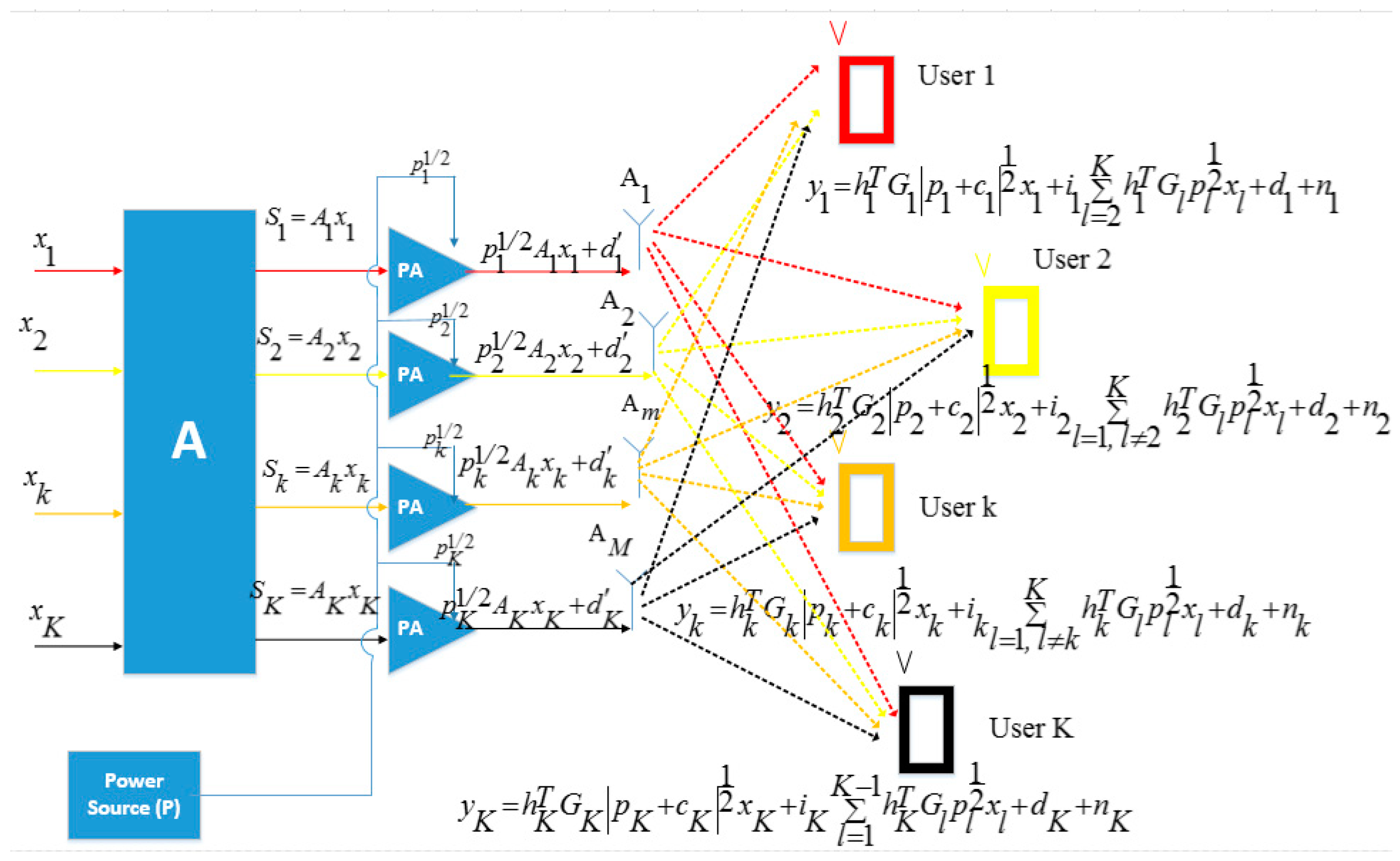
Mathematical expressions of the spectral efficiency and energy efficiency are derived by considering the effects of nonlinear amplifiers in each transmitter branch under the perfect and imperfect channel conditions.

(3)

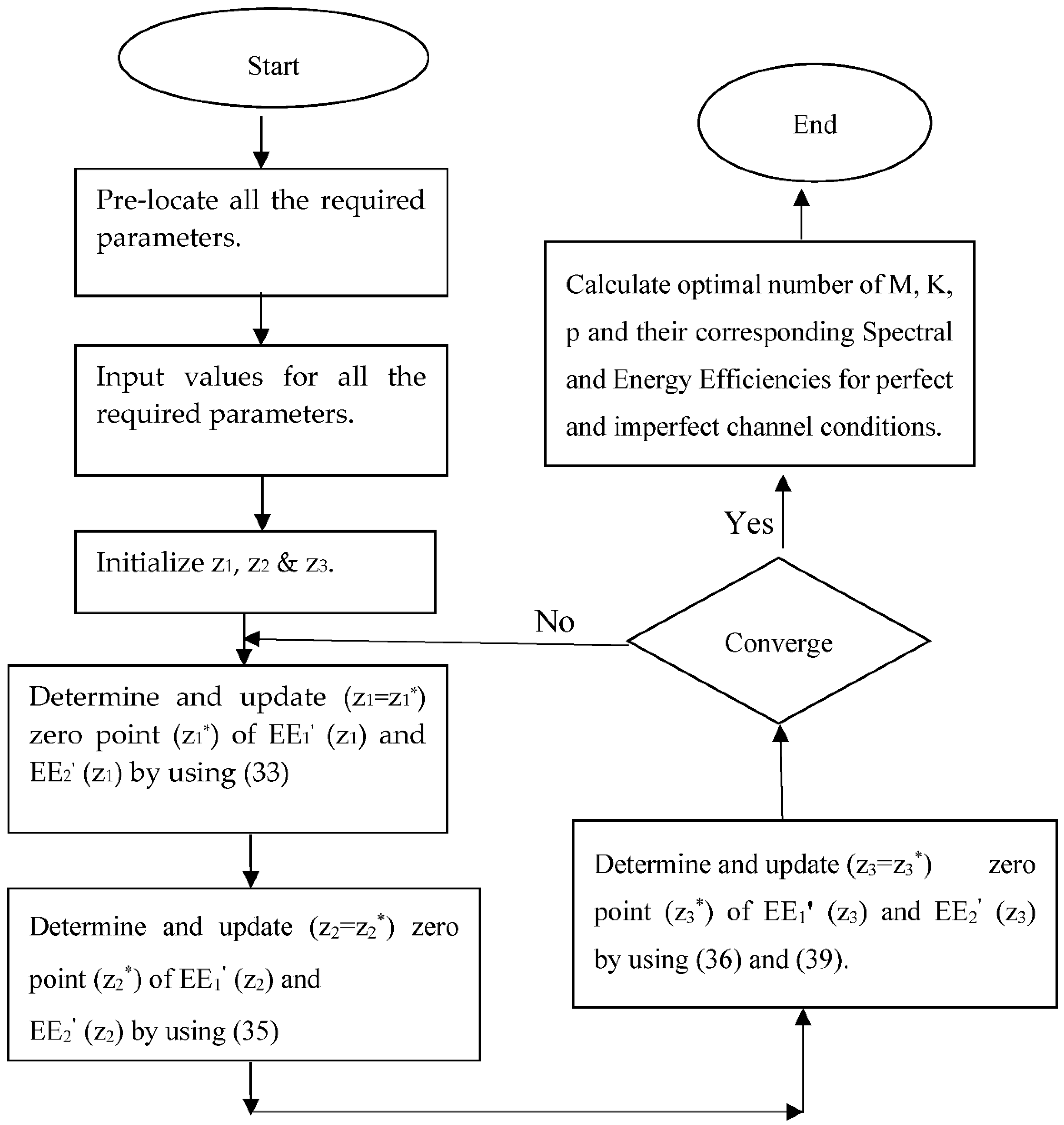
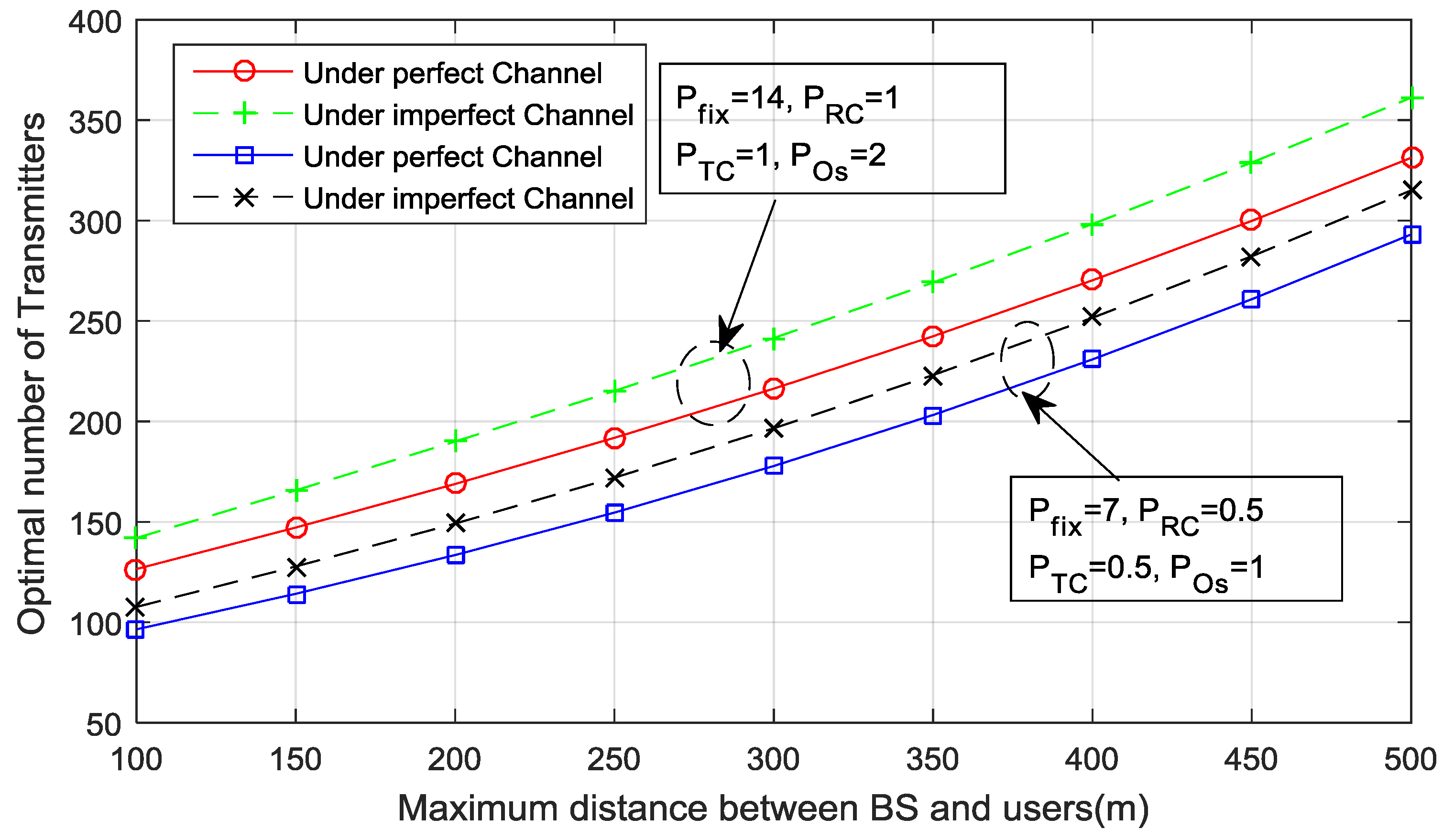
A numerical approach is proposed to optimize the energy efficiency and calculation of optimal parameters. Simulation results are provided to support the mathematical modelling and investigate the relevant trend.

The remainder of the paper is organized as follows: In Section 2 we have discussed the frame structure and working of Massive MIMO, modeled the transmission and reception of signals and derived the achievable rates of Massive MIMO by considering the effects of nonlinear amplifiers under both perfect and imperfect channel conditions. In Section 3, we have modeled the power consumptions of Massive MIMO starting from transmitter end to user terminal. In Section 4, we have defined the problem definition and energy efficiency of Massive MIMO under the perfect and imperfect channel situations. In Section 5, we have modeled the power amplifiers and in Section 6, we have proposed a numerical algorithm in order to solve the optimization problems discussed in Section 4. Section 7 presents simulation results and discussions, and in Section 8 we conclude and summarize all the discussions.

Notations: ${(.)}^{-1}$, ${(.)}^H$ and ${(.)}^T$ show the inverse, Hermitian and transpose operator respectively, $\mathrm{E}[.]$ means the expectation operation, $\mathit{ln}\left(x\right)$ and ${\mathit{log}}_2\left(x\right)$ denote the logarithm of x to base $e$ and $2$ respectively, ${\mathrm{Z}}_{+}$ denotes the set of positive integers, and ${(.)}^{\prime }$ shows the differentiation.

2. Frame Structure and Achievable Rates of Massive MIMO

In Massive MIMO, base station and users have to send training signals known to both transmitters and receivers in order to achieve channel estimation. Accurate and timely acquisition of channel state information (CSI) is very important because Massive MIMO relies on the frequency response of propagation channel. Time Division Duplex (TDD) operation is preferable in the case of massive MIMO because the overhead factor of channel estimation is not dependent on the number of antennas M as compared to FDD operation where overhead factor is so large due to its dependence on the number of antennas. However, few techniques have been proposed and suggested for having the FDD operation in the case of Massive MIMO [32,33,34,35].

Figure 1 illustrates the frame structure of Massive MIMO in the case of TDD protocol. An uplink and downlink channel are reciprocal to each other in TDD operation and use the same frequency spectrum during the uplink and downlink communications at different time slots. During the uplink operation, each user needs to send training signals or orthogonal pilots to the base station in order to estimate the CSI at the base station for $T_p^{ul}$ channel uses followed by the transmission of data from all K users to BS in the same time-frequency resources for $T_d^{ul}$ channel uses as shown in Figure 1. BS uses the linear precoding to retrieve the signals transmitted from all K users together with channel estimation. In the downlink, BS uses the estimated channel in order to transmit the required signals to the intended users for $T_d^{dl}$ channel uses. Number of transmitters M and users K are required to be same during the uplink and downlink operation in the case of TDD protocol.

2.1. Achievable Rates of Massive MIMO under Perfect CSI

Consider the data symbols $x=\left[x_1,x_2,\dots x_k,\dots x_K\right]$ transmitted by the base station antennas intended for the $K$ number of users as shown in Figure 2 then the transmitted vector $S$ can be written as:

$$S=Ax,$$

(1)

where $A$ is a linear precoding matrix and can be expressed as:

$$A=V{P}^{\frac{1}{2}},$$

(2)

where $V$ is a $M\times K$ beam forming vector and can be described as:

$$V=\{\begin{array}{ll}{G}^{*}& \mathrm{for}\mathrm{MRT}\\ \mathrm{G}{\left(G^{H}G\right)}^{-1}& \mathrm{for}\mathrm{ZF}\\ \mathrm{G}{\left(G^{H}G+\frac{K}{p_r}\right)}^{-1}& \mathrm{for}\mathrm{MMSE}\end{array},$$

and $P=diag\left(p\right)$, where $P={\left[p_1,p_2,p_3,\dots ,p_K\right]}^T$ denotes the power allocation for all users as shown in Figure 2.

According to Bussgang’s theorem [36], we can decompose the output of an amplifier as a sum of two uncorrelated components (input signal and the distortion). Let $d_k$ be the distortion caused by the nonlinear amplifier as shown in Figure 2 then the signal received at the $k^{th}$ user can be expressed as:

$$y_k=h_k^T{G}_k{p}_k^{1/2}{x}_k+{\displaystyle \sum _{l=1,l\ne k}^K{h}_k^T{G}_l{p}_l^{1/2}{x}_l+d_k+n_k}.$$

(3)

The second term in the above equation is due to interference among data symbols and $n_k$ is the Additive White Gaussian Noise (AWGN) having zero mean and unity variance.

Let $i_k=\frac{\mathrm{E}\left[{\left({\displaystyle \sum _{l=1,l\ne k}^K{h}_k^T{G}_l{p}_l{x}_l}\right)}^{*}{d}_k\right]}{p_k}$ is the correlation of $d_k$ on the interference term and $c_k$ are the power losses due to nonlinear amplifier, then Equation (3) can be written as:

$$y_k=h_k^T{G}_k{\left|p_k+c_k\right|}^{1/2}{x}_k+i_k{\displaystyle \sum _{l=1,l\ne k}^K{h}_k^T{G}_l{p}_l^{1/2}{x}_l+d_k+n_k},$$

(4)

where $c_k$ can also be seen as the effect of a nonlinear amplifier to the amplitude of the intended signal which can be termed as ‘clipping’ and in practical situations this contribution is negative, i.e.,

$$\left|p_k+c_k\right|<\left|p_k\right|.$$

The corresponding clipping power $p_c$ at the $k^{th}$ user terminal can be written as:

$$p_c=\frac{p_k+c_k}{p_k}.$$

(5)

The variance of the distortion at the $k^{th}$ user terminal due to the nonlinear amplifier can be written as:

$${\sigma }_k^2=D_k=\frac{\mathrm{E}\left[{\left|d_k\right|}^2\right]}{p_k}.$$

(6)

In order to have the equal rate for all the users, power allocations need to be done in a clever way and by employing a technique from [24]; it can be written as:

$$p_k^{\left(ZF\right)}=p\left(M-K\right),$$

(7)

where $p$ is the received signal to noise ratio and it is considered as an optimization parameter because to optimizing $p$ is equivalent to optimizing $p_k$. Since we know that ZF suppresses the interference, the interference term will be zero:

$$i_k{\displaystyle \sum _{l=1,l\ne k}^K{h}_k^T{G}_l{p}_l^{1/2}{x}_l}=0$$

(8)

By using Equations (7) and (8), Equation (4) can be written as:

$$y_k=h_k^T{G}_k{\left|p\left(M-K\right)+c_k\right|}^{1/2}{x}_k+d_k+n_k.$$

(9)

Additionally, the corresponding signal to noise ratio for the $k^{th}$ user ($SN{R}_k$) can be computed as:

$$SN{R}_k=\left(\frac{p\left(M-K\right)+c_k}{D_k+1}\right).$$

(10)

The corresponding achievable rates for the $k^{th}$ user can be defined as:

$$R_k=\left[{\mathit{log}}_2\left(1+SN{R}_k\right)\right],$$

(11)

$$R_k=\mathrm{E}\left[{\mathit{log}}_2\left(1+\left(\frac{p\left(M-K\right)+c_k}{D_k+1}\right)\right)\right].$$

(12)

By considering the over-head factor, achievable rate for the $k^{th}$ user can be expressed as:

$$R_k=\left(1-\frac{T_{sum}K}{U}\right)\mathrm{E}\left[{\mathit{log}}_2\left(1+\left(\frac{p\left(M-K\right)+c_k}{D_k+1}\right)\right)\right],$$

(13)

where the factor $\left(1-\frac{T_{sum}K}{U}\right)$ accounts for the pilot over-head in each coherence block U and $T_{sum}$ is the total relative pilot length.

2.2. Achievable Rates of Massive MIMO under Imperfect CSI

In this subsection, we have calculated the achievable rate of Massive MIMO under imperfect channel conditions. Perfect channel conditions mean that the BS knows all the frequency components of the channel which results in improvement in the performance of the system. In practical situations, due to infinite precision of the electronic instruments and instantaneous nature of the transmission, achieving a perfect CSI is almost impossible. Imperfect CSI causes the inevitable interference among the users which in turn affects the performance of the system. We have assumed that the average attenuation (${\beta }_k$) between the users and base station antennas is inversely proportional to transmission power of each user and for the $k^{th}$ user it will be ($\frac{p{\alpha }^2}{{\beta }_k}$). As explained in Section 2, the transmission is divided into two phases, i.e., pilot transmission followed by data transmission.

During the pilot transmission phase, variance of the estimated channel by using MMSE estimator can be written as [37,38,39]:

$${\sigma }_{h_k^{^}}^2=\frac{{\beta }_k}{1+\frac{1}{pK{T}_p}}.$$

During the data transmission phase, achievable rates for the $k^{th}$ user by assuming the ZF and treating the estimated channel as true channel, considering the effects of a nonlinear amplifier under imperfect channel conditions, can be written as:

$$R_{k,im}=\mathrm{E}\left[{\mathit{log}}_2\left(1+\left(\frac{p\left(M-K\right)+c_k}{D_k+1+\frac{1}{T_p}+\frac{1}{pK{T}_p}}\right)\right)\right],$$

(14)

where $T_p$ is the same as that of $T_p^{ul}$ and, similarly, achievable rates for the $k^{th}$ user by considering the pilot overhead can be expressed as:

$$R_{k,im}=\left(1-\frac{T_{sum}K}{U}\right)\mathrm{E}\left[{\mathit{log}}_2\left(1+\left(\frac{p\left(M-K\right)+c_k}{D_k+1+\frac{1}{T_p}+\frac{1}{pK{T}_p}}\right)\right)\right].$$

(15)

3. Modeling of Power Consumptions

In this section we have modeled the power consumptions of Massive MIMO. The total power consumptions in the circuit of Massive MIMO can be composed into two parts:

$$P_{Tot}=P_{P.A}+P_{C.P},$$

(16)

where $P_{P.A}$ is the total power consumed by the power amplifiers and can be illustrated as [14]:

$$P_{P.A}=\frac{\delta KpB{\alpha }^2}{{\eta }_{PA}},$$

(17)

where $\delta$ is the path loss factor and when the required SNR will be fixed then this factor would be very important in order to calculate the total power consumption of the power amplifiers. ${\eta }_{PA}$ is the efficiency of the power amplifier and is explained in detail in the power amplifier modeling section (Section 5) and $B$ is the bandwidth.

$P_{C.P}$ is the total circuit power consumptions of Massive MIMO, i.e., power consumed in the transmitter and receiver chains, oscillator and filter power consumption, power required for the coding and decoding of the desired signals, power required for the channel estimation and linear processing. So, we need to model all the required or consumed power in the above mentioned processes.

Power consumed at the transmitter and receiver chain can be illustrated as:

$$P_{PTR}=M\left[P_{TC}\right]+K\left[P_{RC}\right]+P_{Os},$$

(18)

where $P_{PTR}$ is the total power consumption at the transmitter and receiver chains, $P_{TC}$ is the power consumption at the transmitter chain, $P_{RC}$ is the power consumption at the receiver chain, i.e., power consumed at the filters, converters and mixers, and $P_{Os}$ is the oscillator power in order to synchronize the frequencies.

The power required for the coding and decoding of the desired signal can be demonstrated as:

$$P_{c/d}=R_K\left(P_c+P_d\right),$$

(19)

where $P_c$ and $P_d$ denote the corresponding power consumption during coding and decoding.

As explained in Section 2, Massive MIMO relies on CSI of the channel, i.e., BS and users have to send training or pilot signals during the uplink and downlink of the channel in order to get the frequency response of the channel during the coherence time. Power consumption during this process can be written as [40]:

$$P_{ce}=\frac{2B}{U}\left[\frac{T^{ul}{K}^{2}M}{{\gamma }_{bs}}+\frac{2T^{dl}{K}^2}{{\gamma }_{ue}}\right],$$

(20)

where ${\gamma }_{bs}$ and ${\gamma }_{ue}$ are the computation efficiencies at the transmitter and receiver end.

Consumption of power during linear processing by assuming ZF has been explained in [24] and can be written as:

$$P_{ZF}=\frac{BK}{U{\gamma }_{bs}}\left(\frac{K^2}{3}+M\left(3K+1\right)\right).$$

(21)

So the total circuit power consumption of Massive MIMO by using Equations (18)–(21) can be expressed as:

$$P_{C.P}=P_{fix}+P_{PTR}+P_{ce}+P_{ZF},$$

$$P_{C.P}=P_{fix}+M\left[P_{TC}\right]+K\left[P_{RC}\right]+P_{Os}+\frac{2B}{U}\left(\frac{T^{ul}{K}^{2}M}{{\gamma }_{bs}}+\frac{2T^{dl}{K}^2}{{\gamma }_{ue}}\right)+\frac{BK}{U{\gamma }_{bs}}\left(\frac{K^2}{3}+M\left(3K+1\right)\right),$$

(22)

where $P_{fix}$ is the fixed power required for site cooling and the total power consumptions Equation (16) of Massive MIMO by using Equation (17), Equation (22) can be illustrated as:

$$P_{Tot}=\frac{\delta KpB{\alpha }^2}{{\eta }_{PA}}+P_{fix}+M\left[P_{TC}\right]+K\left[P_{RC}\right]+P_{Os}+\frac{2B{K}^2}{U}\left(\frac{T^{ul}M}{{\gamma }_{bs}}+\frac{2T^{dl}}{{\gamma }_{ue}}\right)+\frac{BK}{U{\gamma }_{bs}}\left(\frac{K^2}{3}+M\left(3K+1\right)\right).$$

Total power consumptions can be written in more simplified and concentrated way:

$$P_{Tot}=\frac{\delta KpB{\alpha }^2}{{\eta }_{PA}}+{\displaystyle \sum _{i=0}^3{D}_i{K}^i}+M{\displaystyle \sum _{i=0}^2{E}_i{K}^i},$$

(23)

with the following substitutions:

$$\begin{array}{l}{D}_0=P_{fix}+P_{Os},D_1=P_{RC},D_2=\frac{4B{T}^{dl}}{U{\gamma }_{ue}},D_3=\frac{B}{3U{\gamma }_{bs}}\\ E_0=P_{TC},E_1=\frac{B}{U{\gamma }_{bs}},E_2=\frac{3B}{U{\gamma }_{bs}}+\frac{2B}{U{\gamma }_{bs}}\end{array}.$$

4. Energy Efficiency and Problem Formation

The energy efficiency of Massive MIMO can be defined as the spectral efficiency divided by the transmitted and the consumed power. As defined above, spectral efficiency of the system can be written as:

$$R_K=B{\displaystyle \sum _{k=1}^K{R}_k}.$$

where the total power can be written as the algebraic sum of transmitted and consumed power in the circuit of Massive MIMO as defined in the previous section on power modeling (Section 3). So, Energy Efficiency (E.E) can be written as:

$$\mathrm{E}.\mathrm{E}=\frac{B{\displaystyle \sum _{k=1}^K{R}_k}}{P_{P.A}+P_{C.P}}.$$

(24)

In the following subsections, we have calculated and formulated the problem of energy efficiency maximization under perfect and imperfect CSI.

4.1. Energy Efficiency under Perfect CSI

As described in Section 2, the spectral efficiency of Massive MIMO when the channel is perfectly known and by considering the effects of nonlinear power amplifiers can be written as:

$$R_K=\frac{K}{\mathit{ln}\left(2\right)}\left(1-\frac{T_{sum}K}{U}\right)B\left[\mathit{ln}\left(1+\left(\frac{p\left(M-K\right)+c_k}{D_k+1}\right)\right)\right].$$

The average total power as explained in the previous section can be written as:

$$P_{Tot}=\frac{\delta KpB{\alpha }^2}{{\eta }_{PA}}+{\displaystyle \sum _{i=1}^3{D}_i{K}^i}+M{\displaystyle \sum _{i=0}^2{E}_i{K}^i}.$$

So, the energy efficiency when the channel is perfectly known can be written as:

$$\mathrm{E}{.\mathrm{E}}_1=\frac{\frac{K}{\mathit{ln}\left(2\right)}\left(1-\frac{T_{sum}K}{U}\right)B\left[\mathit{ln}\left(1+\left(\frac{p\left(M-K\right)+c_k}{D_k+1}\right)\right)\right]}{\frac{\delta KpB{\alpha }^2}{{\eta }_{PA}}+{\displaystyle \sum _{i=1}^3{D}_i{K}^i}+M{\displaystyle \sum _{i=0}^2{E}_i{K}^i}}.$$

(25)

We need to maximize the energy efficiency of Massive MIMO and in order to maximize the energy efficiency, consider the following mathematical optimization problem:

$$\begin{array}{l}\mathrm{Maximize}{\mathrm{EE}}_1\left(M,K,p\right)\\ \begin{array}{cc}\hfill \mathrm{Constraint}\mathrm{to}:& M\in Z_{+},K\in Z_{+}\hfill \\ & M>K,p>0\hfill \end{array}\end{array}.$$

As the number of BS antennas and users cannot be negative, they have been set positive in the first two constraints of optimization problem and the third constraint is the basic condition that holds for Massive MIMO (number of antennas are greater than number of users).

4.2. Energy Efficiency under Imperfect CSI

In this subsection, we have calculated the energy efficiency under imperfect channel conditions which results in inevitable interference among users. The spectral efficiency under the imperfect channel conditions as explained in Section 2 can be written as:

$$R_{K,im}=\frac{K}{\mathit{ln}\left(2\right)}\left(1-\frac{T_{sum}K}{U}\right)B\left[\mathit{ln}\left(1+\left(\frac{p\left(M-K\right)+c_k}{D_k+1+\frac{1}{T_p}+\frac{1}{pK{T}_p}}\right)\right)\right].$$

So, the corresponding energy efficiency (E.E₂) under the imperfect channel conditions can be written as:

$$\mathrm{E}{.\mathrm{E}}_2=\frac{\frac{K}{\mathit{ln}\left(2\right)}\left(1-\frac{T_{sum}K}{U}\right)B\left[\mathit{ln}\left(1+\left(\frac{p\left(M-K\right)+c_k}{D_k+1+\frac{1}{T_p}+\frac{1}{pK{T}_p}}\right)\right)\right]}{\frac{\delta KpB{\alpha }^2}{{\eta }_{PA}}+{\displaystyle \sum _{i=1}^3{D}_i{K}^i}+M{\displaystyle \sum _{i=0}^2{E}_i{K}^i}}.$$

(26)

The corresponding optimization problem of energy efficiency maximization under imperfect channel conditions can be illustrated as:

$$\begin{array}{l}\mathrm{Maximize}{\mathrm{EE}}_2\left(M,K,p\right)\\ \begin{array}{cc}\hfill \mathrm{Constraint}\mathrm{to}:& M\in Z_{+},K\in Z_{+}\hfill \\ & M>K,p>0\hfill \end{array}\end{array}.$$

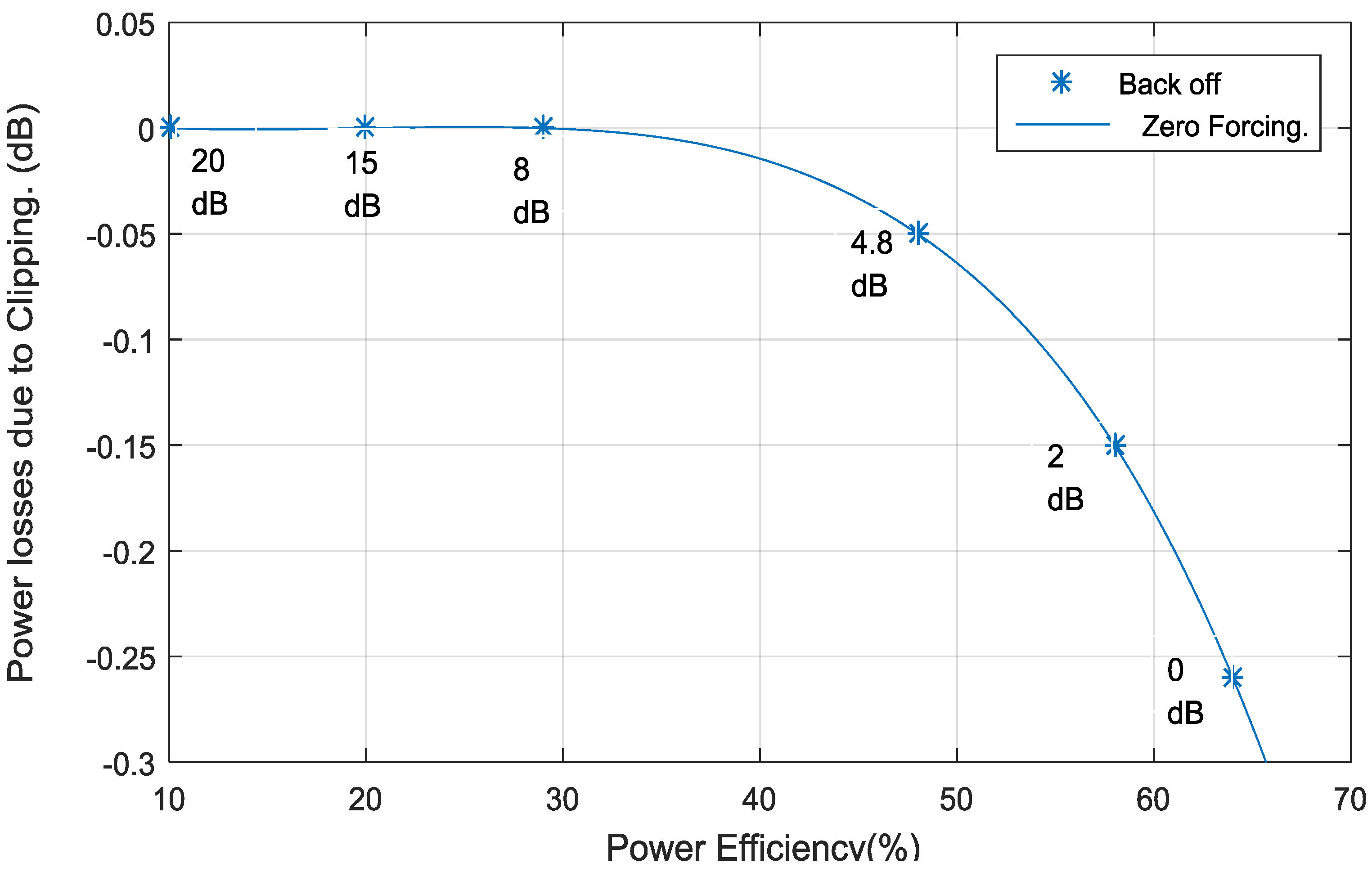
5. Modeling of Nonlinear Amplifiers

Conventionally used amplifiers in the case of MIMO systems are the multi-transistor amplifiers such as Doherty amplifiers. Doherty amplifier splits the input signal into two parts and then amplifies them in two different amplifiers (peaking amplifier and carrier amplifier) and then the outputs of these two amplifiers are summarized to get the desired output. The Doherty amplifier provides higher efficiency and is well suited for the signals which have the higher peak to average power ratios. However, the issues of using the Doherty amplifiers are their higher cost and complexity. Due to these drawbacks, they are not feasible to use in the case of Massive MIMO because of the large number of BS antennas.

We need to have the simple design and cost efficient power amplifiers in the case of Massive MIMO like class A, class B or class C. In this article, we have considered the most basic class B amplifiers and the power efficiency of such kind of amplifier is given as [41]:

$${\eta }_{PA}=\frac{\pi }{4}\left[\frac{\mathrm{E}\left(g^2\left(x\right)\right)}{A_{\mathit{max}}\mathrm{E}\left(g\left(x\right)\right)}\right].$$

(27)

where $g\left(s\right)$ is the AM–AM conversion of the power amplifier. Various models have been proposed and suggested for modeling of power amplifiers in the literature like Solid State Power Amplifier (SSPA) model, Travelling Wave Tube Amplifier (TWTA) model, RAPP model and ERF model. Out of them, the most commonly used is the RAPP model where AM–PM conversion is assumed to be negligible and AM–AM conversion is given by [41]:

$$g\left(x\right)=A_{\mathit{max}}\left[\frac{x/x_{\mathit{max}}}{{\left(1+{\left(\frac{x}{x_{\mathit{max}}}\right)}^{2p}\right)}^{\frac{1}{2p}}}\right],$$

(28)

where p controls the smoothness of the curve and in order to keep the total power P, $x_{\mathit{max}}$ and $A_{\mathit{max}}$ are assumed to be [42]:

$$x_{\mathit{max}}=\sqrt{\mathrm{E}\left[{\left|x_1+x_2+\dots +x_M\right|}^2\right]}=M^{-1/2},$$

(29)

$$A_{\mathit{max}}=x_{\mathit{max}}\left[\frac{\sqrt{P}}{{\epsilon }_o}\right],$$

(30)

where ${\epsilon }_o$ is the compensation factor for the power loses. In the next section, we have developed an algorithm in order to solve the optimization problems of ${\mathrm{EE}}_1$ and ${\mathrm{EE}}_2$.

6. Problem Solution and Numerical Algorithm

In this section, we have designed an algorithm to solve the optimization problems ${\mathrm{EE}}_1$ and ${\mathrm{EE}}_2$. It is difficult to solve the optimization problem of ${\mathrm{EE}}_1$ and ${\mathrm{EE}}_2$ due to mixed nature of their corresponding objective functions with respect to M, K and p. Consider the following substitutions in order to simplify the objective functions of ${\mathrm{EE}}_1$ and ${\mathrm{EE}}_2$:

$$z_1=K,z_2=M/K,z_3=Kp,$$

where $z_1$ can be explicated as the number of active users, $z_2$ can be explicated as the number of active antennas per user and $z_3$ along with multiplication of some constant factor as described in Equation (17) can be explicated as the total power of power amplifiers. The simplified objective functions of ${\mathrm{EE}}_1$ under perfect channel conditions can be written as:

$$\mathrm{E}{.\mathrm{E}}_1=\frac{\frac{z_1}{\mathit{ln}\left(2\right)}\left(1-\frac{T_{sum}{z}_1}{U}\right)B\left[\mathit{ln}\left(1+\left(\frac{z_3\left(z_2-1\right)+c_k}{D_k+1}\right)\right)\right]}{\frac{z_3\delta B{\alpha }^2}{{\eta }_{PA}}+{\displaystyle \sum _{i=1}^3{D}_i{z}_1^i}+z_2{\displaystyle \sum _{i=0}^2{E}_i{z}_1^{i+1}}},$$

(31)

with the following modified optimization problem:

$$\begin{array}{l}\mathrm{Maximize}{\mathrm{EE}}_1\left(z_1,z_2,z_3\right)\\ \mathrm{Constraint}\mathrm{to}:z_1>0,z_2>1\\ z_3>0\end{array}.$$

Similarly, objective function of energy efficiency under imperfect channel conditions following the above mentioned substitutions can be written as:

$$\mathrm{E}{.\mathrm{E}}_2=\frac{\frac{z_1}{\mathit{ln}\left(2\right)}\left(1-\frac{T_{sum}{z}_1}{U}\right)B\mathit{ln}\left(1+\left(\frac{z_3\left(z_2-1\right)+c_k}{D_k+1+\frac{1}{T_p}+\frac{1}{z_3{T}_p}}\right)\right)}{\frac{\delta z_{3}B{\alpha }^2}{{\eta }_{PA}}+{\displaystyle \sum _{i=1}^3{D}_i{z}_1^i}+z_2{\displaystyle \sum _{i=0}^2{E}_i{z}_1^{i+1}}},$$

(32)

with the following modified optimization problem:

$$\begin{array}{l}\mathrm{Maximize}{\mathrm{EE}}_2\left(z_1,z_2,z_3\right)\\ \mathrm{Constraint}\mathrm{to}:z_1>0,z_2>1\\ z_3>0\end{array}.$$

Objective functions of optimization problems ${\mathrm{EE}}_1$ and ${\mathrm{EE}}_2$ follows a quasi-concave response because they are first increasing and then deceasing in each dimension while the other dimensions are fixed and their second order derivatives are less than zero. The proof of the quasi-concave nature of objective functions (${\mathrm{EE}}_1$ and ${\mathrm{EE}}_2$) have been shown in the Appendix A and Appendix B respectively.

According to Appendix A and Appendix B, objective functions ${\mathrm{EE}}_1$ and ${\mathrm{EE}}_2$ undergo a peak point at the unique zero crossing of ${\mathrm{EE}}_1^{\prime }$ and ${\mathrm{EE}}_2^{\prime }$ in each dimension while the other dimensions are fixed. The following flow chart summarizes the above mentioned discussions and shows the simulation steps (Figure 3).

7. Simulations and Numerical Results

In this section, we have performed simulations to test the mathematical and numerical algorithm discussed in the earlier sections. Realistic simulation parameters have been chosen for simulations as shown in the

Table 1. Simulation parameters.

Parameter	Value
Transmission Bandwidth ($B$)	20 MHz
Coherence Block ($U$)	1800
Computational efficiency at BSs (${\gamma }_{bs}$)	$12.8\mathrm{Gflops}/\mathrm{W}$
Computational efficiency at Users (${\gamma }_{ue}$)	$6\mathrm{Gflops}/\mathrm{W}$
Clipping power Loses ($c_k$)	$-0.15\mathrm{dB}$
Path loss exponent ($\alpha$)	3.8
Distortion ($D_k$)	−25 dB
Total Noise Power ($B{\alpha }^2$)	−96 dBm
Pilot Lengths ($T_p$,$T_{sum}$)	1 m, 2m
Power Amplifier Efficiency when fixed (${\eta }_{PA}$)	0.34

. Figure 4 shows the amount of power lost due to clipping at different efficiencies of power amplifier with respect to different back-offs, calculated by using Equations (5), (27) and (28).

Number of transmitters and receivers are set to be 120 and 20 and it can be seen from Figure 4 that the power losses due to the consequences of clipping are less than −0.3 dB.

Similarly, Figure 5 shows the losses due to distortion at different efficiencies of power amplifier with respect to different back-offs. The number of transmitters and receivers and path loss exponent are set to be same in Figure 4 and Figure 5. Figure 6 shows the optimal number of transmitters at different area of coverage ranges from 100 m to 500 m by setting different circuit power consumption levels under both the perfect and imperfect channel conditions As can be seen from Figure 6, when the coverage area increases, the optimal number of transmitters increases, respectively, in order to cover that area and when the channel condition is imperfect then more numbers of transmitters are required, whereas when the power consumptions of the circuit are less, optimal numbers of transmitters required for the system are less and vice versa.

Similarly, Figure 7 shows the optimal number of users at different area of coverage ranges from 100 m to 500 m at different circuit power consumption levels under both the perfect and imperfect channel situations. As can be seen from the Figure 7, more users can be accommodated at a higher area of coverage. Figure 8 shows the optimal transmitted or PA power at different area of coverage ranges from 100 m to 500 m by setting different circuit power consumption levels under both the perfect and imperfect channel conditions.

As can be seen from Figure 8, more transmitted power is required in order to cover more distance and imperfect channel condition results in more transmitted power with the corresponding area throughput that maximizes the energy efficiency of Massive MIMO shown in Figure 9. Figure 10 shows the optimal energy efficiency and it can be seen from Figure 10 that less power consumptions of the circuit results in more achievable energy efficiency and under imperfect channel conditions energy efficiency is reduced because the system need to transmit more transmitted or PA power in order to mitigate the negative effects of imperfect channel conditions.

Figure 11 and Figure 12 show the 3D representation of energy efficiency along with all the optimal parameters in which maximum distance is set to be 300 m and power consumption parameters are set to be $P_{fix}=14$, $P_{TC}$ = 1, $P_{RC}$ = 1 and $P_{Os}$ = 2 under both the perfect and imperfect channel conditions respectively. The optimal parameters come out to be M = 216, K = 112, $P_{P.A}$ = 141.4 W, EE = 19.5 Mbit/Joule whereas energy efficient area throughput to be 11.9 Gbits/Km² in the case of perfect channel conditions as shown in Figure 11 and when the channel conditions are not perfectly known then the optimal parameters comes out to be M = 241, K = 127, $P_{P.A}$ = 245 W, EE = 16.1 Mbit/Joule and area through put = 11.2 Gbits/Km² as shown in Figure 12.

Figure 13 shows the convergence of energy efficiency with respect to the number of iterations by using the numerical algorithm (discussed in Section 6) at various distances under the perfect and imperfect channel conditions. The computation complexity of the proposed algorithm at each iteration can be written as:

$$\mathrm{Computation} \mathrm{Complexity} \mathrm{at} \mathrm{each} \mathrm{iteration} = \mathrm{O}\left(z_1^4\right)+\mathrm{O}\left(z_2\mathit{ln}\left(1+z_2\right)\right)+\mathrm{O}\left(z_3\mathit{ln}\left(z_3\right)\right),$$

where $\mathrm{O}\left(z_1^4\right)$ represents the required computation complexity during the computation of $z_1$, and $\mathrm{O}\left(z_2\mathit{ln}\left(1+z_2\right)\right)$ and $\mathrm{O}\left(z_3\mathit{ln}\left(z_3\right)\right)$ represent the required computation complexity during the computation of $z_2$ and $z_3$ respectively at each iteration. As can be seen from the Figure 13, the energy efficiency converges completely at the sixth iteration, thus the overall computation complexity of the proposed algorithm can be written as $6\left[\mathrm{O}\left(z_1^4\right)+\mathrm{O}\left(z_2\mathit{ln}\left(1+z_2\right)\right)+\mathrm{O}\left(z_3\mathit{ln}\left(z_3\right)\right)\right]$. The power consumptions parameters in Figure 13 are set to be $P_{fix}=7$, $P_{TC}$ = 0.5, $P_{RC}$ = 0.5 and $P_{Os}$ = 1.

Figure 14 shows the impacts of power amplifier efficiencies on the energy efficiency of Massive MIMO and it can be seen easily that when the power amplifiers are operating at higher efficiency, energy efficiency is maximum and vice versa under both perfect and imperfect channel conditions. The power consumptions parameters are set to be $P_{fix}=7$, $P_{TC}$ = 0.5, $P_{RC}$ = 0.5 and $P_{Os}$ = 1 for simulations in Figure 14.

8. Conclusions

This paper mainly focused on the energy efficiency of Massive MIMO by considering the effects of nonlinear amplifiers. The impact of nonlinear amplifiers is investigated on the energy efficiency of massive MIMO along with calculation of optimal parameters by using the proposed alternative algorithm under both the perfect and imperfect channel conditions at different circuit power consumptions. Contrary to the existing work, we used a realistic circuit power consumption model that shows the dependence of circuit power consumption on the number of transmitters and users. We have seen that when the channel conditions are not perfectly known, then the system needs to transmit more power in order to overcome the negative effects of imperfect channel situations, and, owing to more transmitted PA power, the energy efficiency gets reduced as compared to the situation when the channel is perfectly known. Numerical results do not change much for a small change in the circuit power consumption but can otherwise change drastically. The alternative algorithm that we have used for joint calculation of optimal parameters works efficiently and converges quickly. Simulations result shows that when the power amplifiers are working at higher efficiency, then the energy efficiency of Massive MIMO also is increased, while it is better to have large cell coverage in the case of Massive MIMO along with less circuit power consumptions. In future, circuit power consumptions will be reduced, resulting in further improved energy efficiency with less transmitted or PA power, together with improved and simpler signal processing. The combination of energy efficient massive MIMO along with nonlinear amplifiers can be a fascinating option for low cost future wireless systems.

References

1. Thomas, M.; Larsson, E.G.; Yang, H. Hien Quoc Ngoet, 1st ed.; Fundamentals of Massive MIMO, Cambridge University Press: Cambridge, MA, USA, 2016. [Google Scholar]
2. Ramezani, P.; Jamalipour, A. Toward the evolution of wireless powered communication networks for the future Internet of Things. IEEE Netw. 2018, 6, 62–69. [Google Scholar] [CrossRef]
3. Caire, G.; Jindal, N.; Kobayashi, M.; Ravindran, N. Multiuser MIMO achievable rates with downlink training and channel state feedback. IEEE Trans. Inf. Theory 2010, 56, 2845–2866. [Google Scholar] [CrossRef]
4. Jose, J.; Ashikhmin, A.; Marzetta, T.L.; Vishwanath, S. Pilot contamination and precoding in multi-cell TDD systems. IEEE Trans. Wirel. Commun. 2011, 10, 2640–2651. [Google Scholar] [CrossRef]
5. Verdú, S. Multiuser Detection; Cambridge University Press: Cambridge, MA, USA, 1998. [Google Scholar]
6. Viswanath, P.; Tse, D.N.C. Sum capacity of the vector Gaussian broadcast channel and uplink-downlink duality. IEEE Trans. Inf. Theory 2003, 49, 1912–1921. [Google Scholar] [CrossRef]
7. Weingarten, H.; Steinberg, Y.; Shamai, S. The capacity region of the Gaussian multiple-input multiple-output broadcast channel. IEEE Trans. Inf. Theory 2006, 52, 3936–3964. [Google Scholar] [CrossRef]
8. Li, Q.; Li, G.; Lee, W.; Lee, M.I.; Mazzarese, D.; Clerckx, B.; Li, Z. Mimo techniques in wimax and lte: A feature overview. IEEE Commun. Mag. 2010, 48, 86–92. [Google Scholar] [CrossRef]
9. Hanzo, L.; Akhtman, Y.; Wang, L.; Jiang, M. MIMO-OFDM for LTE, WiFi and WiMAX: Coherent versus Non-coherent and Cooperative Turbo Transceivers; IEEE Press and John Wiley & Sons: New York, NY, USA, 2010. [Google Scholar]
10. Marzetta, T.L. Noncooperative cellular wireless with unlimited numbers of BS antennas. IEEE Trans. Wirel. Commun. 2010, 9, 3590–3600. [Google Scholar] [CrossRef]
11. Björnson, E.; Larsson, E.G.; Marzetta, T.L. Massive MIMO: Ten myths and one critical question. IEEE Commun. Mag. 2016, 54, 114–123. [Google Scholar] [CrossRef]
12. Kamga, G.N.; Xia, M.; Assa, S. Spectral-Efficiency Analysis of Regular- and Large-Scale (Massive) MIMO with a Comprehensive Channel Model. IEEE Trans. Veh. Technol. 2017, 66, 4984–4996. [Google Scholar] [CrossRef]
13. Xu, J.; Li, S.; Qiu, L.; Slimane, B.S.; Yu, C. Energy efficient downlink MIMO transmission with linear precoding. Sci. Chin. Inf. Sci. 2013, 56, 1–12. [Google Scholar] [CrossRef]
14. Larsson, E.G.; Richter, F.; Fehske, A.J.; Fettweis, G.P. Energy efficiency aspects of base station deployment strategies for cellular networks. In Proceedings of the 2009 IEEE 70th Vehicular Technology Conference Fall (VTC 2009-Fall), Anchorage, AK, USA, 20–23 September 2009. [Google Scholar]
15. Yang, Y.; You, X.; Juntti, M.; Wang, C.; Leib, H.; Ding, Z. Guest editorial spectrum and energy efficient design of wireless communication networks: Part, I. IEEE J. Sel. Areas Commun. 2013, 31, 825–828. [Google Scholar] [CrossRef]
16. Min, R.; Chandrakasan, A. A Framework for Energy-Scalable Communication in High-Density Wireless Networks. In Proceedings of the 2002 international symposium on Low power electronics and design (ISLPED ‘02), Monterey, CA, USA, 12–14 August 2002; pp. 36–41. [Google Scholar]
17. Cui, S.; Goldsmith, A.J.; Bahai, A. Energy-efficiency of MIMO and cooperative MIMO techniques in sensor networks. IEEE J. Sel. Areas Commun. 2004, 22, 1089–1098. [Google Scholar] [CrossRef]
18. He, A.; Srikanteswara, S.; Reed, J.H.; Chen, X.; Tranter, W.H.; Bae, K.K.; Sajadieh, M. Minimizing energy consumption using cognitive radio. In Proceedings of the IEEE International Performance, Computing and Communications Conference, Austin, TX, USA, 7–9 December 2008. [Google Scholar]
19. He, A.; Srikanteswara, S.; Bae, K.K.; Newman, T.R.; Reed, J.H.; Tranter, W.H.; Sajadieh, M.; Verhelst, M. System power consumption minimization for multichannel communications using cognitive radio. In Proceedings of the IEEE International Conference on Microwaves, Communications, Antennas and Electronics Systems, Tel Aviv, Isreal, 9–11 November 2009. [Google Scholar]
20. Cui, S.; Goldsmith, A.J.; Bahai, A. Energy constrained modulation optimization. IEEE Trans. Wirel. Commun. 2005, 4, 2349–2360. [Google Scholar]
21. Gao, S.; Qian, L.; Vaman, D.R.; Qu, Q. Energy efficient adaptive modulation in wireless cognitive radio sensor networks. In Proceedings of the IEEE International Conference on Communications, Glasgow, Scotland, 24–28 June 2007. [Google Scholar]
22. Kim, H.S.; Daneshrad, B. Energy-aware link adaptation for MIMO OFDM based wireless communication. In Proceedings of the IEEE Military Communications Conference (MILCOM 2008), San Diego, CA, USA, 16–19 November 2008. [Google Scholar]
23. Mohammed, E.S. Impact of transceiver power consumption on the energy efficiency spectral efficiency tradeoff of zero-forcing detector in massive MIMO systems. IEEE Trans. Commun. 2014, 62. [Google Scholar] [CrossRef]
24. Björnson, E.; Sanguinetti, L.; Hoydis, J.; Debbah, M. Optimal Design of Energy-Efficient Multi-User MIMO Systems: Is Massive MIMO the Answer? IEEE Trans. Wirel. Commun. 2015, 14, 3059–3075. [Google Scholar] [CrossRef]
25. Xu, W.; Li, S.; Feng, Z.; Vasilakos, A.V. Joint Parameter Selection for Massive MIMO: An Energy-Efficienct Perspective. IEEE Access 2016, 4, 3719–3731. [Google Scholar] [CrossRef]
26. Guerreiro, J.; Dinis, R.; Montezuma, P. Massive MIMO with Nonlinear Amplification: Signal Characterization and Performance Evaluation. In Proceedings of the 2016 IEEE Global Communications Conference, San Diego, CA, USA, 4–8 December 2016. [Google Scholar] [CrossRef]
27. Studer, C.; Larsson, E. PAR-aware large-scale multi-user MIMOOFDM downlink. IEEE J. Sel. Areas Commun. 2013, 31, 303–313. [Google Scholar] [CrossRef]
28. Mohammed, S.; Larsson, E. Per-antenna constant envelope precoding for large multi-user MIMO systems. IEEE Trans. Commun. 2013, 61, 1059–1071. [Google Scholar] [CrossRef]
29. Emil, B. Massive MIMO systems with non-ideal hardware: Energy efficiency, estimation, and capacity limits. IEEE Trans. Inf. Theory 2014, 60, 7112–7139. [Google Scholar]
30. Hien Quoc, N.; Larsson, E.G.; Marzetta, T.L. Energy and spectral efficiency of very large multiuser MIMO systems. IEEE Trans. Commun. 2013, 61, 1436–1449. [Google Scholar] [CrossRef]
31. Jiang, F.; Chen, J.; Swindlehurst, A.L.; López-Salcedo, J.A. Massive MIMO for Wireless Sensing with a Coherent Multiple Access Channel. IEEE Trans. Signal Process. 2015, 63, 3005–3017. [Google Scholar] [CrossRef]
32. Rao, X.; Lau, V.K. Distributed compressive CSIT estimation and feedback for FDD multi-user massive MIMO systems. IEEE Trans. Signal Process. 2014, 62, 3261–3271. [Google Scholar]
33. Choi, J.; Love, D.; Bidigare, P. Downlink training techniques for FDD massive MIMO systems: Open-loop and closed-loop training with memory. IEEE J. Sel. Top. Signal Process. 2014, 8, 802–814. [Google Scholar] [CrossRef]
34. Jiang, Z.; Molisch, A.; Caire, G.; Niu, Z. Achievable rates of FDD massive MIMO systems with spatial channel correlation. IEEE Trans. Wirel. Commun. 2015, 14, 2868–2882. [Google Scholar] [CrossRef]
35. Choi, J.; Chance, Z.; Love, D.; Madhow, U. Noncoherent trelliscoded quantization: A practical limited feedback technique for massive MIMO systems. IEEE Trans. Commun. 2013, 61, 5016–5029. [Google Scholar] [CrossRef]
36. Rowe, H. Memoryless nonlinearities with Gaussian input: Elementary results. Bell Syst. Tech. J. 1982, 61, 1519–1526. [Google Scholar] [CrossRef]
37. Bj¨ornson, E.; Ottersten, B. A framework for training-based estimation in arbitrarily correlated Rician MIMO channels with Rician disturbance. IEEE Trans. Signal Process. 2010, 58, 1807–1820. [Google Scholar] [CrossRef]
38. Ciuonzo, D.; Rossi, P.S.; Dey, S. Massive MIMO channel-aware decision fusion. IEEE Trans. Signal Process. 2015, 63, 604–619. [Google Scholar] [CrossRef]
39. Amirpasha, S.; Dey, S.; Ciuonzo, D.; Rossi, P.S. Massive MIMO for Decentralized Estimation of a Correlated Source. IEEE Trans. Signal Process. 2016, 64, 2499–2512. [Google Scholar]
40. Khan, A.A.; Uthansakul, P.; Uthansakul, M. Energy Efficiency Design of Massive MIMO by incorporating with Mutual Coupling. Int. J. Commun. Antenna Propag. 2017, 7. [Google Scholar] [CrossRef]
41. Ochiai, H. An analysis of band-limited communication systems from amplifier efficiency and distortion prospective. IEEE Trans. Commun. 2013, 61, 1460–1472. [Google Scholar] [CrossRef]
42. Mollen, C.E.; Larsson, G.; Erikson, T. On the impact of PA-Induced In-Band Distortion in Massive MIMO. In Proceedings of the 20th European Wireless Conference, Spain, 14–16 May 2014. [Google Scholar]
Figure 1. Frame structure of Massive Multiple-Input Multiple-Output (MIMO) in the case of TDD protocol.
Energies 11 01045 g001
Figure 2. Block diagram of Massive MIMO with nonlinear amplifiers.
Energies 11 01045 g002
Figure 3. Alternative numerical algorithm for solving the optimization problem.
Energies 11 01045 g003
Figure 4. Clipping power losses at different back-offs and power efficiencies.
Energies 11 01045 g004
Figure 5. Distortion loses at different back-offs and power efficiencies.
Energies 11 01045 g005
Figure 6. Optimal number of transmitters at different area of coverages.
Energies 11 01045 g006
Figure 7. Optimal number of receivers at different area of coverages.
Energies 11 01045 g007
Figure 8. Optimal Power of non-linear amplifiers.
Energies 11 01045 g008
Figure 9. Area throughput.
Energies 11 01045 g009
Figure 10. Energy efficiency (EE) at different area of coverages.
Energies 11 01045 g010
Figure 11. 3-D representation of EE along with optimal parameters under perfect channel situation.
Energies 11 01045 g011
Figure 12. 3-D representation of EE along with optimal parameters under Imperfect channel situation.
Energies 11 01045 g012
Figure 13. Convergence of energy efficiency.
Energies 11 01045 g013
Figure 14. Energy efficiency at different distortion level and power amplifier efficiencies.
Energies 11 01045 g014