Article

A Three-Dimensional Radiation Transfer Model to Evaluate Performance of Compound Parabolic Concentrator-Based Photovoltaic Systems

Education Ministry Key Laboratory of Advanced Technology and Preparation for Renewable Energy Materials, Yunnan Normal University, Kunming 650500, China
*
Author to whom correspondence should be addressed.
Energies 2018, 11(4), 896; https://doi.org/10.3390/en11040896
Submission received: 11 March 2018 / Revised: 3 April 2018 / Accepted: 9 April 2018 / Published: 11 April 2018

Abstract

:
In the past, two-dimensional radiation transfer models (2-D models) were widely used to investigate the optical performance of linear compound parabolic concentrators (CPCs), in which the radiation transfer on the cross-section of CPC troughs is considered. However, the photovoltaic efficiency of solar cells depends on the real incidence angle instead of the projection incidence angle, thus 2-D models can’t reasonably evaluate the photovoltaic performance of CPC-based photovoltaic systems (CPVs). In this work, three-dimensional radiation transfer (3-D model) within CPC-θa/θe, the CPC with a maximum exit angle θe for radiation within its acceptance angle (θa), is investigated by means of vector algebra, solar geometry and imaging principle of plane mirror, and effects of geometry of CPV-θa/θe on its annual electricity generation are studied. Analysis shows that, as compared to similar photovoltaic (PV) panels, the use of CPCs makes the incident angle of solar rays on solar cells increase thus lowers the photovoltaic conversion efficiency of solar cells. Calculations show that, 2-D models can reasonably predict the optical performance of CPVs, but such models always overestimate the photovoltaic performance of CPVs, and even can’t predict the variation trend of annual power output of CPV-θa/θe with θe. Results show that, for full CPV-θa/θe with a given θa, the annual power output increases with θe first and then comes to a halt as θe > 83°, whereas for truncated CPV-θa/θe with a given geometric concentration (Ct), the annual power output decreases with θe.

1. Introduction

In recent years, solar photovoltaic systems have attracted much attention for electricity generation due to the gradual depletion of traditional fossil fuels and severe environmental issues caused by their use [1]. However, the high cost of the electricity produced by PV systems still limits their broader worldwide application. In China, the cost of electricity generated by PV systems was about 0.12–0.15 $/kWh in 2016, two times of the cost of electricity generated by conventional electricity generation technologies, and the enterprises have to rely on subsides from governments to survive. Concentrating solar radiation onto a photovoltaic can reduce the solar area per unit output, thus allowing the cost of the total system to be reduced per unit of energy delivered. Concentrated PV systems are divided into high concentration PV systems (HCPVs) and low concentration PV systems (LCPVs). HCPVs are usually equipped with sophisticated devices for tracking the Sun and cooling the solar cells [2,3], but LCPVs are simple in the structure and easy to control and hence more attractive. A study by Mallick and Eames showed that, compared to similar PV panels, a LCPV can reduce the cost of electricity by up to 40% [4]. Due to the advantages of non-tracking, high reliability and low-cost, various types of low solar concentrators were developed and tested for the use with solar cells in the past two decades. Among these, the compound parabolic concentrator (CPC) was regarded as to be most suitable and efficient low concentrator.
Mallick and Eames developed an asymmetric CPV with a geometric concentration of 2.01 for building integration in Europe, and a 62% increase in power output was measured as compared to similar PV panel [5,6]. Brogren et al. experimentally tested a CPC with a geometric concentration ratio of 3 for concentrating solar radiation on Cu(In, Ga)Se2 solar cells, and found that the use of CPC increased the maximum power output of the solar cells by 90% [7]. A comparative study by Yousef et al. under hot and arid climatic conditions showed that, in comparison with similar solar panels, the electricity generated by CPC (2.4×)-based CPV system with and without cooling of solar cells was 52% and 33% higher, respectively [8]. Bahaidarah et al. experimentally investigated the performance of CPC-based PV/T systems with and without glazing and concluded that the use of glass reduced the power output and thus was recommended for higher thermal gain, and the unglazed system was suitable for greater electric power output [9]. Stationary CPCs are commonly oriented in the east-west direction with a yearly fixed tilt angle for efficient solar radiation concentration [10], therefore, the increase in electricity from reflective CPVs is limited due to limited geometric concentration. In order to increase the geometric concentration of CPCs, dielectric totally internally reflecting compound parabolic concentrators (DCPCs) were suggested by Rabl and Winston [11]. Muhammad-Sukki et al. experimentally investigated the performance of a mirror symmetrical dielectric totally internally reflecting CPC (4.9×)-based photovoltaic system for building applications, and found that the use of DCPC made the maximum electrical power output point increase by a factor of 4.2 [12]. Theoretically, the use of a CPC should make the power output of solar cells increase by the factor of its geometric concentration, but the actual increase is much less than this value, a result of the optical loss due to multiple reflections of solar rays on the way to the solar cells and electricity loss mainly resulting from lower photovoltaic conversion efficiency due to higher cell temperature, non-uniform irradiation and increased solar incidence angle [13]. To make the distribution of solar radiation on solar cells more uniform, Su and Li et al. proposed a lens-walled CPC, and such CPC shares the advantages of high optical efficiency, large acceptance angle, and low cost as compared to reflective CPCs and dielectric CPCs [14,15]. A CPC-based PV system with rolling mark on the reflectors was tested by Hatwaambo et al., and found that the use of semi-diffuse reflectors slightly but insignificantly improved the performance of the PV system [16,17]. However, a study by Yu and Tang showed that the use of semi-diffuse reflectors in CPVs can’t noticeably improve the uniformity of solar flux distribution except when reflectors with perfect diffuse reflection are employed, which in turn results in a great reduction of annually collected radiation [17]. To simply the fabrication of CPC- based PV systems and make radiation distribution on solar cells more uniform, a compound plane mirror concentrator (CPC-A) was investigated as an alternative to CPC by Tang et al., who found that the annually radiation collected by optimized CPC-As and CPCs is almost identical [18].
It is well known that the incidence angle and cell temperature have a significant effect on the photovoltaic conversion efficiency of solar cells [19,20]. To ensure LCPVs operate efficiently, their cooling is required and the heat removed from solar cells can be used for other thermal applications; such CPC-based PV/T systems were widely investigated in the past [21,22,23]. Recently, Baig et al. theoretically and experimentally investigated the performance of a crossed compound parabolic concentrator-based PV system (CCPC) with a thermal extraction unit, and found that such a system had an average electrical efficiency of 10–16% when evaluated at five different locations [24]. However, the effect of solar incidence angle on the photovoltaic performance of CPVs was rarely investigated. The incidence angle of solar rays reflecting from the parabolic reflectors of CPVs gradually increases from the upper tip downwards to the lower end, and radiation reflecting from the parabolic reflector near solar cells is very large, hence can’t be efficiently converted into electricity output [25]. The earlier work by Rabl and Winston indicated that the use of CPCs with a restricted exit angle (CPC-θa/θe) can improve the photovoltaic performance of CPVs thanks to the limited solar incident/exit angle [26]. For CPC-θa/θe, the solar incidence angle on the absorber is limited within θe for the radiation within its acceptance angle (θa), and common CPC, the one without restriction of exit angle, is a special case of CPC-θa/θe for θe = 90° [27]. An comparative study conducted by Yu et al. showed that, in comparison with CPV-20/90, power output increases of 2.1%, 5.4% and 8.17% from CPV-20/65 were measured for projected incident angle θp = 0°, 10° and 16°, respectively. Yu also found that, for a CPV-θa/θe, the solar flux distribution on solar cells had an insignificant effect on the power output, but the solar incident angle had a significant effect [28].
For linear CPCs, the projected angles of incident and reflected rays (all projected angles mentioned in this work is the angle of projection of solar rays on the cross-section of the CPC-trough relative to the normal of the CPC’s aperture) are identical [29], therefore theoretical analysis on the optical performance based on radiation transfer on cross-section of CPCs (2-D model) is reasonable, hence its wide use in the past. Recently, Yu et al. proposed a 2-D model to investigate the annual power output of CPV-θa/θe based on the angular distribution of annual collectible radiation, and found that, with increase of θe, the annual electricity generated by E-W CPV-θa/θe decreased, except full CPV-θa/θe with the aperture’s tilt-angle being yearly adjusted four times at three tilts [27]. However, the solar incident angle mentioned in the paper is the projection angle, but the efficiency of solar cells is dependent on the real solar incidence angle [28,30]. Therefore, to reasonably evaluate the photovoltaic performance of CPVs, a three-dimensional radiation transfer model is required. Theoretically, using three-dimensional ray tracing analysis to investigate the long-term performance of CPVs is feasible, but not practical due to the numerous ray-tracing analyses necessary to find the angular dependence of the photovoltaic efficiency of solar cells on both real and projected incident angles because of time variation of the sun’ position over the sky dome in a day and daily variation of the Sun’s declination [31]. In this work, a trial is first made to suggest a mathematical procedure to find the real solar incidence angle of all radiation on solar cells of CPV-θa/θe for solar radiation from any direction of the sky based on three-dimensional radiation transfer within CPVs (3-D model) by means of vector algebra, convenient but powerful, solar geometry as well imaging principle of plane mirror. The objective of this work is to study the effect of θe on the annual electricity generation from CPV-θa/θe as well the reasonability of the 2-D model proposed by Yu [27] for evaluating the performance of CPVs.

2. Optical and Photovoltaic Conversion Efficiency of CPVs
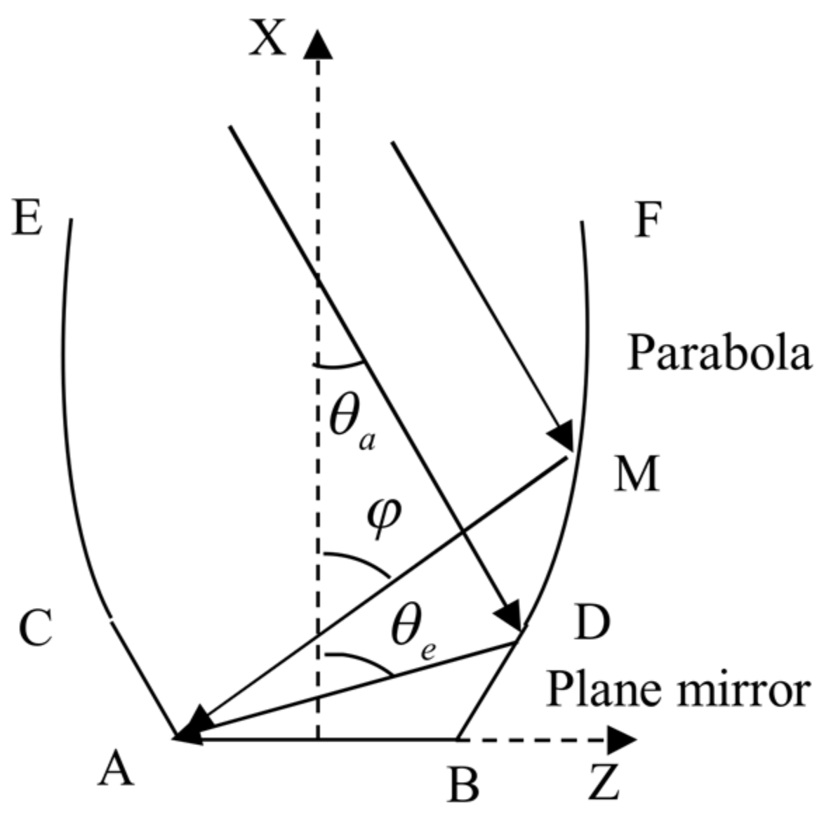
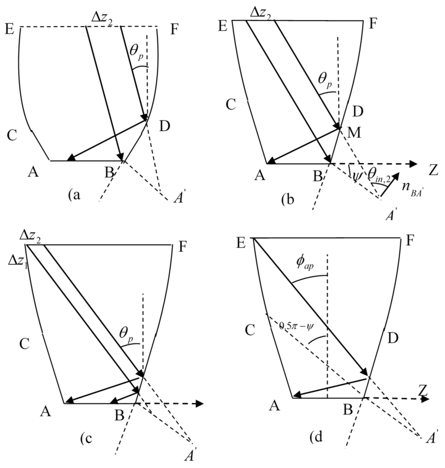
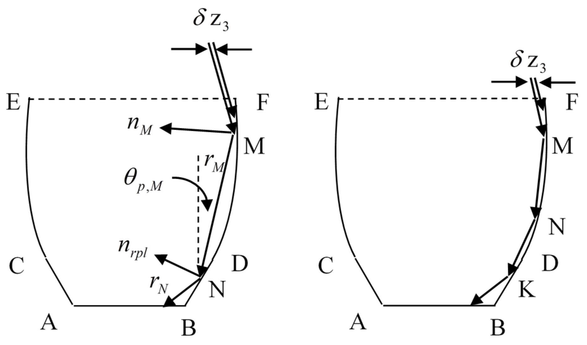
2.1. Equation of Reflectors of CPC-θae

As shown in Figure 1, CPC-θa/θe consists of an upper parabola and lower plane mirrors. To make analysis easier and convenient, the width of the absorber/solar cell of the CPVs is set to be 1, and the right parabola in the Cartesian coordinates system shown in Figure 1 is expressed by Equation (1):
{ z = ( sin θ e + sin θ a ) sin ϕ 1 cos ( ϕ + θ a ) 0.5 x = ( sin θ e + sin θ a ) cos ϕ 1 cos ( ϕ + θ a ) ( θ t ϕ θ e )
where ϕ is the polar angle of any point on the parabolic reflector relative to the x-axis; θa the acceptance half-angle, θt the edge-ray angle of CPC-θa/θe after being truncated with a geometric concentration ratio of Ct. For full CPC-θa/θe, θt = θa and Ct = sinθe/sinθa; whereas for truncated CPCs with a given Ct, the θt is calculated based on Equation (1) [25]. Obviously, the CPC-θa/90, the one without restriction of exit angle, is a special case of CPC-θa/θe for θe = 90°. The plane mirror of CPC-θa/θe is expressed by:
x = c tan γ p l ( z 0.5 ) ( 0.5 z z D )
and γpl, the tilt-angle of plane mirrors relative to the x-axis, is given by Equation (3) [27]:
γ p l = 0.5 ( θ e θ a )
The terms zD and xD are the z- and x- component of the lower end (D) of the right parabola, respectively, and calculated from Equation (1) by setting ϕ = θe.

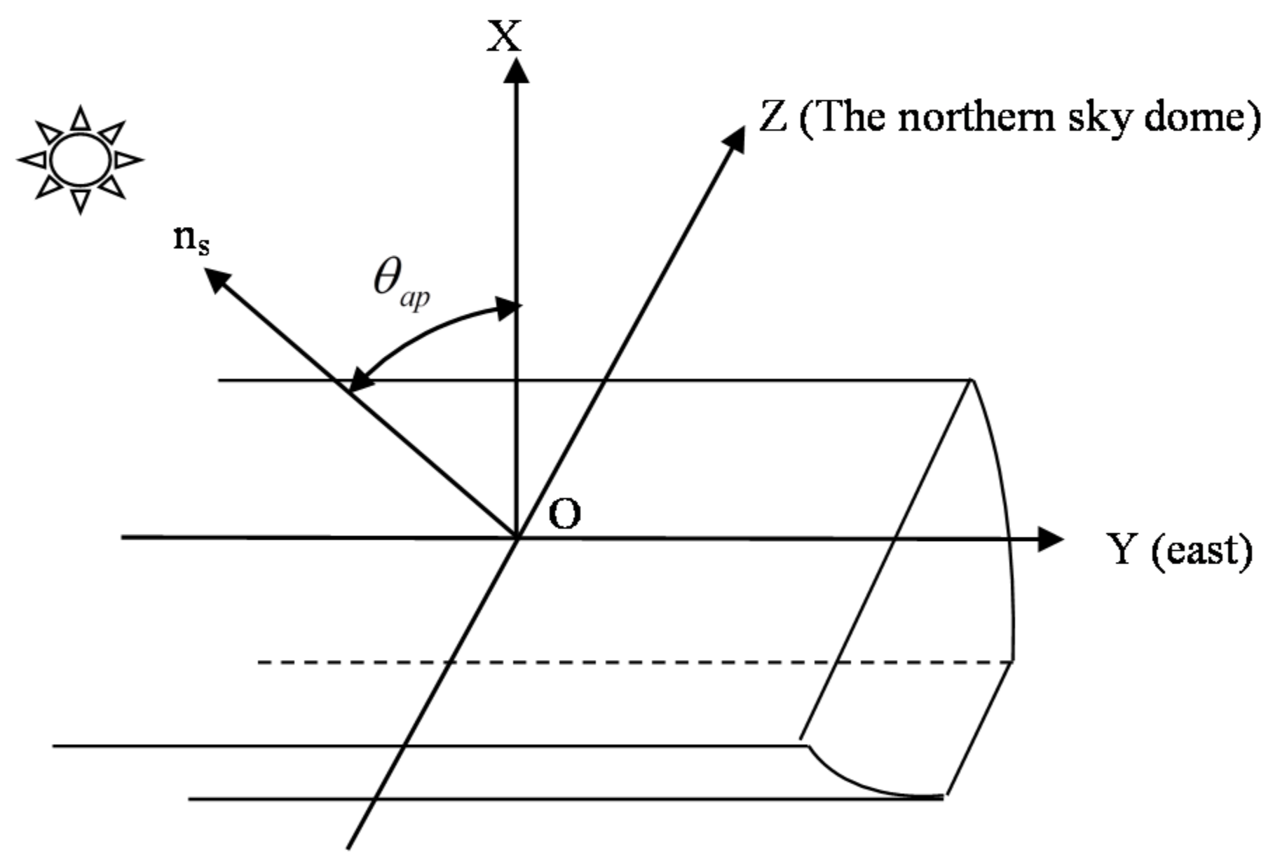
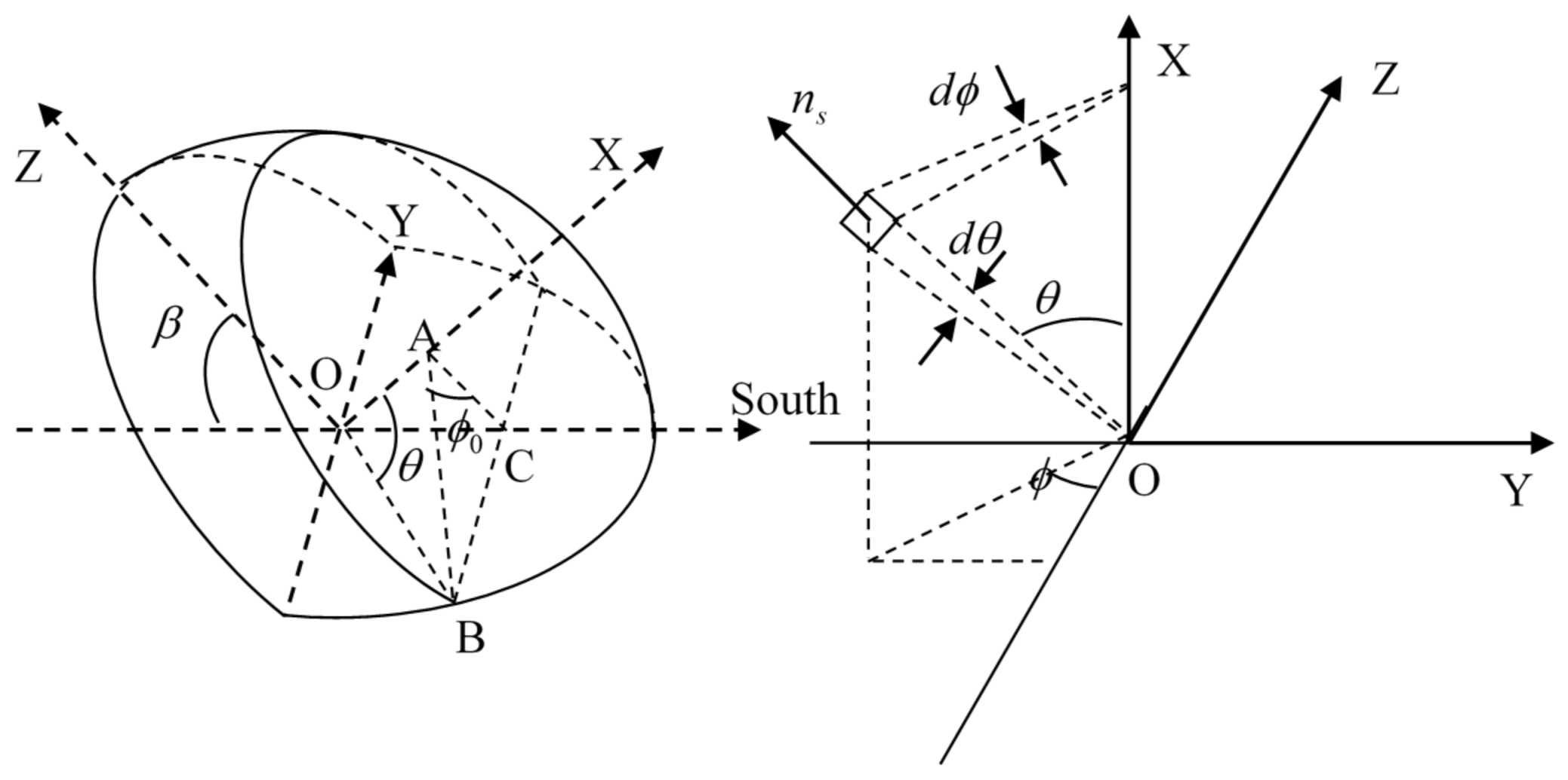
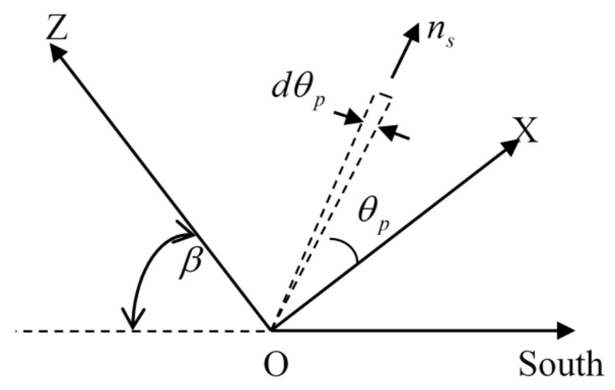
2.2. Coordinate System to Determine the Vector of Solar Rays

CPC-troughs are usually oriented in the east-west direction with the aperture tilted at β from the horizon. For analysis convenience, a coordinate system with the x-axis normal to the aperture, y-axis pointing to east and z-axis pointing to northern sky is introduced (see Figure 2). The unit vector of incident solar ray at any time of a day in this coordinate system is expressed [31,32]:
n s = ( n x , n y , n z )
where:
n x = cos δ cos ω cos ( λ β ) + sin δ sin ( λ β )
n y = cos δ sin ω
n z = cos δ cos ω sin ( λ β ) + sin δ cos ( λ β )
where λ is the site latitude, ω the solar hour angle, and δ the declination of the Sun which vary with day number counted from the first day of a year [31]. The irradiation situation within linear CPCs is uniquely determined by the projected angle of incident rays (θp), and is given by Equation (6):
tan θ p = | n z n x |
For symmetric CPCs, the optical and photovoltaic performance for ns = (nx, ny, ±nz) are identical. Thus, to make the analysis convenient and simple, the vector of the incident solar radiation at any time is set to be ns = (nx, ny, − |nz|), i.e., in this work solar rays are assumed to be always incident towards onto the right reflector of CPCs (see Figure 3).

2.3. Photovoltaic Conversion Efficiency of Solar Cells

In general, the electricity from a CPV is affected by many factors such as cell temperature and electric load [33]. To simplify the analysis but make our comparative study of the electricity from different CPVs meaningful, it is assumed that, except for the solar incidence angle (θin), the effects of all other factors on the photovoltaic efficiency of CPVs with different geometry are identical, and the photovoltaic efficiency of solar cells is subjected to the following correlation, suggested based on experimental measurements of PV panel under outdoor conditions by Yu et al. [28]:
η p v = 15.5494 + 0.02325 θ i n   0.00301 θ i n 2 + 9.4685   ×   10 5 θ i n 3   1.134   ×   10 6 θ i n 4 ( 0 < θ i n <   65 ° )
η p v =   41.52     0.4784 θ i n ( 65 ° < θ i n <   90 ° )

2.4. Optical and Photovoltaic Conversion Efficiency of CPVs

For CPV-θa/θe, the incidence angle of solar rays reflecting from different parts, even different points of reflectors, is different. For convenience of the analysis, the radiation on solar cells is divided into six parts: radiation directly irradiating on solar cells (I1), radiation incident on right plane mirror and arriving on solar cells after reflection (I2), radiation incident on right parabolic reflector and arriving on solar cells after multiple reflections (I3), radiation on upper right parabola at θp > θa and arriving on solar cells after reflection from parabola first then from left mirror (I4), radiation on left mirror and arriving on solar cells after reflection (I5) and that incident on left parabola and arriving on solar cells after multiple reflections (I6). Hence, the optical efficiency factor of CPV-θa/θe is given by:
f = I 1 + I 2 + I 3 + I 4 + I 5 + I 6 I a p = f 1 + f 2 + f 3 + f 4 + f 5 + f 6
where Iap is the radiation on the aperture of CPVs; fi (i = 1, 2, 3, 4, 5, 6) is the energy fraction of the radiation on solar cells contributed by Ii. Similarly, the photovoltaic conversion efficiency of CPV-θa/θe can be expressed by:
η = P 1 + P 2 + P 3 + P 4 + P 5 + P 6 I a p = η 1 + η 2 + η 3 + η 4 + η 5 + η 6
where Pi (i = 1, 2, 3, 4, 5, 6) is the power output from CPVs due to the contribution of Ii, and the ηi (i = 1, 2, 3, 4, 5, 6) is the photovoltaic conversion efficiency of CPVs contributed by Pi.

2.4.1. Calculation of f1 and η1

As seen from Figure 3, the solar cell of CPVs is fully directly irradiated as θpγf and partially irradiated as γf < θpθt, thus, the energy fraction of the radiation directly irradiating on solar cells of CPVs is simply expressed by f1 = I1/Iap = Δz1/Ct as follows:
f 1 = { 1 / C t ( θ p γ f ) 0.5 ( 1 + C t ) ( 1 tan θ p / tan θ t ) / C t ( γ f < θ p θ t ) 0 e l s e
where γf , the angle that the solar cells of CPVs is fully irradiated for θpγf, is calculated by Equation (11):
tanγf = (Ct − 1) tanθt/(Ct + 1)
θin,1, the solar incident angle on solar cells, is given by:
cos θ i n , 1 = n s · n a b s = n s · ( 1 , 0 , 0 ) = n x
where nabs = (1, 0, 0) is the vector of normal to solar cells of CPVs. Therefore, η1 is given by:
η 1 = Δ z 1 η p v ( θ i n , 1 ) / C t = f 1 η p v ( θ i n , 1 )
where ηpv(θin,1), the photovoltaic efficiency of solar cells as the function of θin,1, is estimated by Equation (7).

2.4.2. Calculation of f2 and η2

In this work, CPV-θa/θe with θa < 2θe − 0.5 π is investigated, and for such CPVs, radiation irradiating on plane mirrors will arrive on solar cells after one reflection as indicated by Yu et al. [27]. The imaging principle of plane mirrors indicates that solar rays pointing to solar cells’ image formed by a plane mirror will hit on solar cells after reflection, therefore, for θpθa, all radiation irradiating on the entire right mirror (BD) will strike on the solar cells after reflection (see Figure 4a); for θa < θpθt, the radiation irradiating on lower part of mirror (MB) (see Figure 4b), will redirect onto the solar cells, and for θt < θp < θp,c1, the plane mirror is partially irradiated, thus only radiation irradiating on the middle part of the mirror will redirect onto the solar cells (see Figure 4c), whereas for θp > θp,c1, no radiation arrives on solar cells from the plane mirror (see Figure 4d). Hence, the energy fraction of radiation irradiating on the right mirror and arriving on solar cells after one reflection is given by:
f 2 = Δ z 2 ρ / C t
and:
Δ z 2 = { z D 0.5 + x D tan θ p θ p θ a cos ψ sin ψ tan θ p θ a < θ p θ t ( h t + sin ψ ) ( tan φ a p tan θ p ) θ t < θ p θ p , c 1 0 θ p > θ p , c 1
where ρ is the reflectivity of reflectors; ht = 0.5(Ct + 1)/tanθt the height of CPVs; ψ = 2γpl(θeθa) the opening angle of V-trough formed by two plane mirrors of CPVs; θp,c1 = Min(φap, 0.5πψ) the critical angle, and for radiation at θpθp,c1, no radiation arrives on solar cells from plane mirrors. As shown in Figure 4d, the φap in Equation (14b) is calculated by:
tan φ a p = 0.5 + cos ψ + 0.5 C t h t + sin ψ
The photovoltaic efficiency of CPVs due to contribution of I2 is given by:
η 2 = Δ z 2 ρ η p v ( θ i n , 2 ) / C t = f 2 η p v ( θ i n , 2 )
where θin,2 is the incidence angle of solar rays reflecting from the right plane mirror, and can be directly calculated based on ns and nBA’ = (cosψ, 0, sinψ), the vector of normal to solar cells’ image BA’ (see Figure 4b), as:
cos θ i n , 2 = n s n B A = n x cos ψ + n z sin ψ

2.4.3. Calculation of f3 and η3

As well known, for ideal solar concentration, all solar rays within its acceptance angle (i.e., θpθa) will arrive on solar cells after more than one reflection, but the solar incidence angle on solar cells differs for radiation incident on different point of the parabolic reflectors. Hence, to find the power output of CPVs contributed by I3, the finite element method must be employed. As shown in Figure 5, the radiation incident on a finite element around M of parabola and arriving on solar cells after more than one reflection is given by:
Δ I 3 = δ z 3 η o p t , 3
and δz3 is given by:
δ z 3 =   ( d z + d x tan θ p )
The “-” in Equation (19) is a result of the fact that x- and z-components of point M decrease with ϕM. The ηopt,3 in Equation (18), the optical efficiency of CPVs for radiation irradiating on finite element around M, is dependent on reflection number of solar ray on way to solar cells and can be calculated by the mathematical procedure presented in Appendix A. The power output due to contribution of ΔI3 is as:
Δ P 3 = Δ I 3 η p v ( θ i n , 3 ) = δ z 3 η o p t , 3 η p v ( θ i n , 3 )
where θin,3, the solar incidence angle on cells, is determined by the method in Appendix A. The total radiation received by solar cells is calculated by integrating ΔI3 = δz3ηopt,3 from ϕ = θt to θe, thus f3 is expressed by:
f 3 = ϕ = θ t ϕ = θ e ( d z + d x tan θ p ) η o p t , 3 / C t
Similarly, one has:
η 3 = ϕ = θ t ϕ = θ e ( d z + d x tan θ p ) η o p t , 3 η p v ( θ i n , 3 ) / C t
It must be noted that f3 and η3 are zero for θp > θa because no radiation reflected from the parabola arrives on the solar cells in this case, except for radiation irradiating on the upper (right) parabolic reflector which is included in I4 as discussed in the next section.

2.4.4. Calculation of f4 and η4

As shown in Figure 6, the solar ray striking at tip (F) of right parabola at θp = θp,c2 just redirects to the end (B’) of the solar cells’ image first, then hits at end (B) of the solar cells after two reflections. Hence, solar rays irradiating on upper part (FK) of right parabola at θa < θp < θp,c2 will arrive on solar cells after two reflections [27]. According to the principle that projected angles of incident and reflective rays on the cross-section of CPVs are identical [27], one has:
θ p , c 2 = ϕ a p 2 γ a p
where γap, the tilt-angle of tangent line to parabolic reflectors at the upper tip, is determined by Equation (A2) in Appendix A. As shown in Figure 6, the ϕK of point K, from which solar ray reflecting just points to end B’ of solar cells’ image for θa < θp < θp,c2, is subjected to following equation group:
{ θ p , K = 2 γ K + θ p tan γ K = ( cos θ a cos ϕ K ) / ( sin θ a + sin ϕ K ) tan θ p , K = ( z K + 0.5 + cos ψ ) ( x K + sin ψ )
Given θp and the geometry of CPVs, ϕK can be obtained by iterative calculations from Equation (24). As shown in Figure 6, the radiation incident on the finite element around point M of right parabola and arriving on solar cells after two reflections is calculated by:
Δ I 4 = ( d z + d x tan θ p ) ρ 2
The power output due to contribution of ΔI4 is given by:
Δ P 4 = Δ I 4 η p v ( θ i n , 4 ) = ( d z + d x tan θ p ) ρ 2 η p v ( θ i n , 4 )
where θ i n , 4 , the incident angle on solar cells, is calculated based on r M and n A B = (cos ψ , 0, −sin ψ ), the vector of normal to solar cells’ image ( A B ), as:
cos θ i n , 4 = r M · ( cos ψ , 0 , sin ψ ) = cos θ r , M cos ψ ( n z + 2 cos θ i , M cos γ M ) sin ψ
Substituting Equations (A1) and (A4) in Appendix A into above obtains:
cos θ i n , 4 = n x cos ( ψ + 2 γ M ) + n z sin ( ψ + 2 γ M )
The total radiation that incident on the upper parabola at θ a < θ p < θ p , c 2 and arrive on solar cells, I4, is calculated by integrating Equation (25) from φ = θ t to φ K , hence f 4 is given by:
f 4 = { θ t ϕ K ( d z + d x tan θ p ) ρ 2 / C t ( θ a < θ p < θ p , c 2 ) 0 e l s e
Similarly, one has:
η 4 = { θ t ϕ K ( d z + d x tan θ p ) ρ 2 η p v ( θ i n , 4 ) / C t ( θ a < θ p < θ p , c 2 ) 0 e l s e

2.4.5. Calculation of f 5 and η 5

As seen in Figure 7, the left mirror of CPVs is fully irradiated as θ p γ f d and partially irradiated as γ f d < θ p γ f , hence, energy fraction of radiation irradiating on left plane mirror and arriving on solar cells after reflection is as follows:
f 5 = Δ z 5 ρ / C t
and:
Δ z 5 = { z D 0.5 x D tan θ p θ p γ f d 0.5 ( C t 1 ) h tan θ p γ f d < θ p γ f 0 θ p > γ f
tan γ f d = ( 0.5 C t z D ) / ( h t x D )
The power output of CPVs due to contribution of I 5 = Δ z 5 ρ is calculated by:
P 5 = Δ z 5 ρ η p v ( θ i n , 5 )
Therefore, the photovoltaic efficiency of CPVs due to contribution of P 5 is given by:
η 5 = P 5 / C t = f 5 η p v ( θ i n , 5 )
As seen in Figure 7, the solar incident angle, θ i n , 5 , is calculated based on n s and n A B = (cos ψ , 0, −sin ψ ), the vector of normal to solar cells’ image A B , as:
cos θ i n , 2 = n x cos ψ = n z sin ψ

2.4.6. Calculation of f 6 and η 6

As seen in Figure 8, the left parabola is fully irradiated as θ p γ a p , partially irradiated as γ a p < θ p < γ f d , and fully shaded by itself for θ p γ f d . For radiation incident at γ a p < θ p < γ f d , the lower left parabola is irradiated, and critical point V is subjected to following equation:
tan θ p = ( 0.5 C t z V ) / ( h t x V )
and z V and x V as the function of φ V are subjected to Equation (1). Given θ p and geometry of CPVs, for γ a p < θ p < γ f d , φ V can be obtained from Equation (35), whereas for θ p γ a p , φ V = θ t . For symmetric CPVs, the optical and photovoltaic performance for n s = ( n x , n y , ± n z ) are identical. As seen from Figure 9, given φ M , the radiation incident on a finite element around M of left parabola at θ p and arriving on solar cells after more than one reflections is equal to that incident on a finite element around M of right parabola at − θ p and arriving on solar cells after more than one reflection. Therefore, f 6 and η 6 can be simply obtained based on the method proposed to find f 3 and η 3 by setting θ p = − θ p and n z = | n z | as follows:
f 6 = ϕ = ϕ V ϕ = θ e ( d z d x tan θ p ) η o p t , 6 / C t
η 6 = ϕ = ϕ V ϕ = θ e ( d z d x tan θ p ) η o p t , 6 η p v ( θ i n , 6 ) / C t
where θ i n , 6 and η o p t , 6 are the solar incident angle and optical efficiency of CPVs for solar rays incident on a finite element around M of left parabola, respectively, and calculated based on the method to find θ i n , 3 and η o p t , 3 in Appendix A by setting θ p = − θ p and n z = | n z | in relevant expressions. It must be noted that f 6 and η 6 are zero for the case of θ p γ f d .
The analysis in the above indicates that, given the geometry of CPVs, the optical efficiency of CPVs only depends on θ p because the irradiation situation within CPVs and reflection number of solar rays on their way to the solar cells are uniquely determined by θ p [13], but the photovoltaic efficiency of CPVs is dependent on both θ p and θ a p as the solar incidence angle is dependent on n x and n z . The analysis in the Appendix A shows that the use of CPCs makes the incidence angle on solar cells increase, leading the photovoltaic efficiency of CPVs to decrease in comparison to similar PV panels.

3. Annual Optical and Photovoltaic Performance of CPVs

It is assumed that the CPV- θ a / θ e is oriented in the east-west direction, the length is considered to be infinite, and radiation from the ground is neglected, hence, radiation received by unit area of solar cells at any time of a day is given by:
I = C t I b g ( θ a p ) f cos θ a p + I a b s , d = C t I b g ( θ a p ) n x f + I a b s , d
The electricity generated by unit area of solar cells of CPVs at any time in a day is expressed by:
P = C t I b g ( θ a p ) n x η + P d
where Ib is the intensity of beam radiation, θ a p , subjected to cos θ a p = n x , is the solar incident angle on aperture of CPVs, g ( θ a p ) , being 1 for n x > 0 otherwise zero, a control function. The I a b s , d in Equation (38) is the sky diffuse radiation collected by unit area of solar cells, and P d in Equation (39) is the power output generated by I a b s , d .
To calculate I a b s , d and P d , isotropic sky diffuse radiation is assumed, thus the sky diffuse radiation from a finite element on the sky dome and received by unit area of solar cells (see Figure 10) is:
d I a b s , d = C t i d cos θ f d Ω
The power output generated by d I a b s , d is expressed by:
d P d = C t i d cos θ η d Ω
where d Ω = sin θ d θ d ϕ is the solid angle covered by a finite element on the sky dome, and the vector of sky diffuse radiation from the finite element (see Figure 10) is expressed by:
n s = ( cos θ , sin θ sin ϕ , | sin θ cos ϕ | )
The i d in Equation (41) is the directional intensity of sky diffuse radiation, and can be determined based on the horizontal sky diffuse radiation Id as:
I d = 0 2 π d φ s 0 0.5 π i d cos θ i sin θ i d θ i = π i d
Thus, one has i d = I d / π , and I a b s , d and P d can be respectively calculated by integrating d I a b s , d and d P d over the sky dome viewed from the aperture of CPVs as:
I a b s , d = C t i d sin θ cos θ f d θ d φ
P d = C t i d sin θ cos θ η d θ d φ
As shown in Figure 10, for the sky dome over the aperture, θ varies from 0 to 0.5 π , and ϕ varies from ϕ 0 to 2 π ϕ 0 . For θ 0.5 π β , ϕ 0 = 0; whereas for 0.5 π β < θ 0.5 π , it is given by:
cos ϕ 0 = tan ( 0.5 π β ) tan θ = ctan θ ctan β   ( 0.5 π β < θ π )
Therefore, Equations (44) and (45) can be rewritten as:
I a b s , d = 2 C t I d π φ 0 π d φ 0 0.5 π sin θ cos θ f d θ = C d I d
P d = 2 C t I d π φ 0 π d φ 0 0.5 π sin θ cos θ η d θ = C d , p v I d
where:
C d = 2 C t π φ 0 π d φ 0 0.5 π sin θ cos θ f d θ
C d , p v = 2 C t π φ 0 π d φ 0 0.5 π sin θ cos θ η d θ
Given β , Cd and Cd,pv are constants, and can be calculated by numerical calculations. For similar solar panels without using CPCs, the power output at any time of a day is given by:
P 0 = I b g ( θ a p ) η p v ( θ a p ) n x + C d 0 , p v I d
C d 0 , p v = 2 π φ 0 π d φ 0 0.5 π sin θ cos θ η p v ( θ ) d θ
If two-dimensional sky diffuse radiation is used to calculate I a b s , d and P d , the vector of diffuse radiation from a finite element of sky vault is n s = ( cos θ p , 0, | sin θ p | ) as seen in Figure 11, and I a b s , d is given by:
I a b s , d = C t [ 0 0.5 π i p cos θ p f d θ p + 0 0.5 π β i p cos θ p f d θ p ]   = C d I d
where i p = 0.5Id [13], and C d is given by:
C d = 0.5 [ 0 0.5 π cos θ p f d θ p + 0 0.5 π β cos θ p f d θ p ]
Similarly:
P d = C d , p v I d
C d , p v = 0.5 [ 0 0.5 π cos θ p η d θ p + 0 0.5 π β cos θ p η d θ p ]
Calculations show that C d calculated based on two- and three-dimensional isotropic sky diffuse radiation is completely identical, but C d , p v calculated based on two-dimensional sky diffuse radiation is about 9% higher than that calculated based on three-dimensional sky diffuse radiation as seen in Figure 12. This means that, two-dimensional sky diffuse radiation can be used to estimate the sky diffuse radiation received by solar cells of CPVs, but not suitable for the estimation of P d .
The daily radiation collected by unit area of solar cells of CPVs is estimated by integrating Equation (38) over the daytime as:
H d a y = C t t 0 t 0 I b g ( θ a p ) n x f d t + C d H d
The daily electricity output of CPVs is given by integrating Equation (39) over the daytime:
P d a y = C t t 0 t 0 I b g ( θ a p ) n x η d t + C d , p v H d
For similar PV panels without using CPCs, the daily electricity generation is given by:
P d a y , 0 = t 0 t 0 I b g ( θ a p ) n x η p v ( θ a p ) d t + C d 0 , p v H d
The Hd in the above expressions is the daily sky diffuse radiation on the horizon, t0 is the sunset time on the horizon in the day. At any time of a day, the position of the sun in terms of n s can be determined, then f and η can be calculated. Therefore, given Hd and the time variation of Ib in a day, Hday, Pday and Pday,0 can be numerically obtained, then summing Hday, Pday and Pday,0 in all days of a year yields annual radiation on solar cells (Sa) and annual power output Pa and Pa,0.

4. Numerical Approach

In this work, monthly average daily global radiation on the horizon in Beijing ( λ = 39.95°) was used for calculations [34], and monthly average Hd and time variation of Ib in a day of the month are estimated based on correlations proposed by Collares-Pereira and Rabl [35]. The steps of φ , θ and ϕ for calculating f , η , C d and C d , p v are set to be 0.1°; the time interval for calculating the daily radiation on solar cells and daily power output is set to be 1 min. To fully study the effect of geometry of CPV- θ a / θ e on the performance, CPVs with aperture’s tilt-angle being yearly fixed (1T-CPVs) and yearly adjusted four times at three tilts (3T-CPVs) are considered. For 1T-CPVs, the tilt-angle of CPVs’ aperture ( β ) is taken to be site latitude ( λ ) [10]; whereas for 3T-CPVs, β is set to be λ during the period of 23 days before and after both equinoxes, and adjusted to be λ − 22 and λ + 22 in summers and winters, respectively [13,18]. All calculations are done using Visual Basic coding programmed by the authors based on the mathematical expressions presented in this work.

5. Results and Discussions

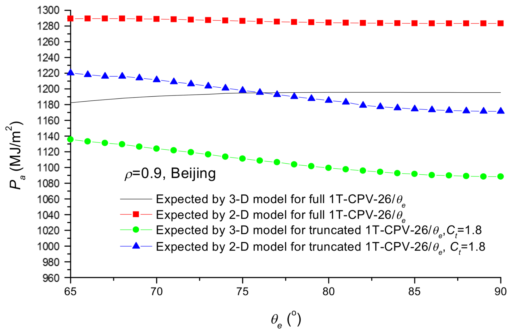
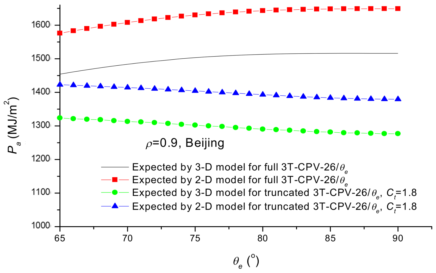
5.1. Annual Collectible Radiation

As seen from Figure 13 and Figure 14, for full CPVs with a given θ a , the annual radiation on solar cells of CPVs increases with the increase of θ e due to the increase of geometric concentration factor; whereas for truncated CPVs with given Ct and θ a , the annual collectible radiation is almost kept unchanged. It is seen from Figure 13 and Figure 14 that the annual collectible radiation expected by the 3-D model is slightly lower than that expected by the 2-D model of Yu [27], and the deviation of Sa expected by 2-D model of Yu from that expected by 3-D model increases with θ e . For full and truncated 1T-CPV-26/ θ e , the maximum deviation is 0.35% and 0.18%, respectively; whereas for full and truncated 3T-CPV-26/ θ e , the maximum deviation is about 0.95% and 0.24%, respectively. This is because the one-reflection model was employed in 2-D model of Yu, and optical loss due to multiple reflections of solar rays on way to solar cells of CPVs is not considered. These results show that 2-D model proposed by Yu et al. [27] can reasonably predict the optical performance of CPVs.
Figure 15 presents comparisons of Sa and Pa of full 3T-CPV-20/ θ e calculated based on the 3-D model of this work incorporated with two-reflection and three-reflection models. It is seen that the deviation of Sa and Pa estimated by two-reflection model from those estimated by three-reflection model are considerably small, and the maximum deviation of Sa and Pa is about 0.18% and 0.26%, respectively. This means that, 3-D model incorporated with two-reflection model can accurately predict the performance of CPVs. Consequently, this work the 3-D model incorporated with three-reflection model is used for calculations.

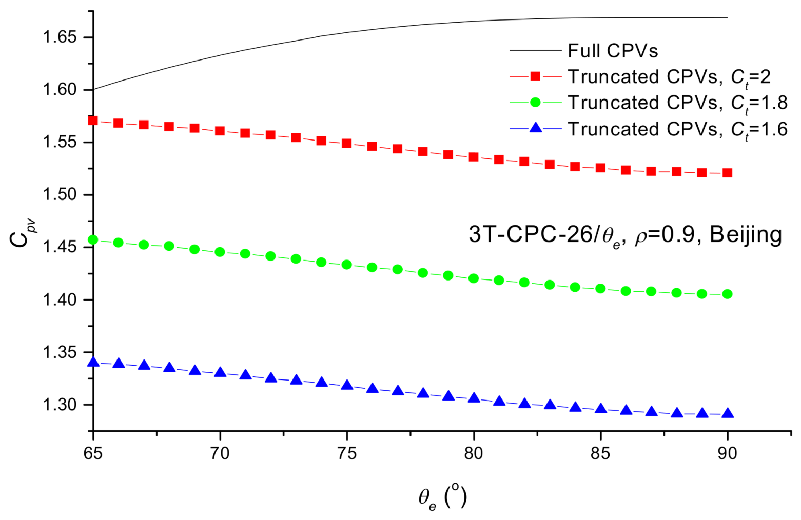
5.2. Annual Photovoltaic Performance of CPVs

Figure 16 presents the effect of θ e on the annual power output of 1T-CPV-26/ θ e in terms of Cpv = Pa/Pa,0, the annual power output increase factor of CPVs as compared to similar PV panel without using CPCs. It is seen that, for full CPV-26/ θ e , the Cpv increases with the increase of θ e first then comes to a halt as θ e > 83°, a result of the fact that the geometric concentration factor of full CPC-26/ θ e increases with θ e but such an increase becomes slow as θ e close to 90°; whereas for truncated CPV-26/ θ e with a given Ct, the Cpv decreases with θ e , a result of the fact that, with the increase of θ e , more radiation will arrive on solar cells at large angles as indicated by Yu [27]. The same situation is also observed for 3T-CPV-26/ θ e as seen in Figure 17.
Figure 18 shows effects of θ e on the annual average photovoltaic efficiency ( η a , p v ) of 1T-CPV-26/ θ e , a ratio of annual power output (Pa) of CPVs to the annual collectible radiation (Sa). As expected, the η a , p v decreases with the increase of θ e because, with the increase of θ e , more radiation arrives on solar cells at larger incident angles [27]. It is also shown that, given θ e and θ a , η a , p v increases with the decrease of Ct because, with the decrease of Ct, more radiation directly irradiates on solar cells, furthermore less radiation is lost due to reflections as multiple reflections usually takes place for radiation irradiating on the upper parabolic reflector. The same situation is also found for 3T-CPVs as shown in Figure 19. It is also seen from Figure 16 and Figure 17 that the Cpv of CPVs is much less than Ct, a result of optical loss due to imperfect reflections and electrical loss due to lower photovoltaic efficiency resulting from increased solar incident angle.
Comparisons of the annual power output from 1T-CPV-26/ θ e expected by 3-D model and the 2-D model of Yu are presented in Figure 20 and Figure 21 in terms of Pa and P a , C P V 26 / θ e / P a , C P V 26 / 90 , the ratio of annual power output from CPV-26/ θ e to that from CPV-26/90. As expected, the annual power output calculated based on the 2-D model are about 7.3–9% higher than those obtained by the 3-D model, and this is attributed to fact that the actual solar incidence angle on solar cells of CPVs is larger than the projected incidence angle which was used to determine the photovoltaic efficiency of solar cells in the 2-D model of Yu, leading the η p v calculated based on the 2-D model to be overestimated. Figure 20 indicates that, for truncated 1T-CPV-26/ θ e , the annual power output expected by both 2-D and 3-D models decreases with the increase of θ e , indicating that the variation trends of Pa with θ e expected by 2-D and 3-D models are in agreement as seen in Figure 21; whereas for full 1T-CPV-26/ θ e , the Pa obtained based on 3-D model increases with θ e , but the Pa expected based on 2-D model of Yu decreases with θ e , indicating that variation trends of Pa with θ e expected by 2-D model of Yu and 3-D model are not in agreement (see in Figure 21).
Comparisons of the annual power output from 3T-CPV-26/ θ e expected by 2-D and 3-D models are presented in Figure 22 and Figure 23. It is seen that, the 2-D model of Yu always overestimates (about 8.3%) the annual power output as compared to the 3-D model, but the variation trend of Pa with θ e expected by 2-D model of Yu agrees with that obtained by the 3-D model for both full and truncated 3T-CPV-26/ θ e . These results indicate that the 2-D model of Yu always overestimates the annual power output of CPVs in comparison to the 3-D model, and even can’t predict the variation trend of Pa with θ e .

6. Conclusions

In this work, a three-dimensional radiation transfer model (3-D model) to predict the performance of CPV- θ a / θ e by means of vector algebra, solar geometry and imaging principle of plan mirrors is suggested, and this model allows one to reasonably investigate the effect of geometry of CPVs on annual radiation collection and power output, thus it is helpful for the design of CPVs. The analysis shows that, for CPV- θ a / θ e with a given geometry, the optical efficiency uniquely depends on the projected angle of incident solar rays ( θ p ), but the photovoltaic efficiency is dependent on θ p and the real incidence angle on the aperture ( θ a p ); and the use of CPCs makes solar incidence angle on solar cells increase thus lowering the photovoltaic efficiency of solar cells in comparison to similar PV panels. Calculations show that the two-dimensional radiation transfer model can reasonably predict the optical performance of CPVs, but such a model always overestimates (by about 7.3–9%) the photovoltaic performance of CPVs in comparison to the 3-D model, and even can’t predict the variation trend of annual power output of CPV- θ a / θ e with θ e . The results indicate that, for full CPV- θ a / θ e , the annual power output increases with θ e first and then comes to a halt as θ e > 83°; whereas for truncated CPV- θ a / θ e , the annual power output always decreases with θ e . The method presented in this work also can be used to investigate the performance and design optimization of other linear concentrating PV systems.

Acknowledgments

This work is partial fulfillment of funded program 51466016, financially supported by Nature Science Foundation of China.

Author Contributions

Runsheng Tang was the supervisor of the work; Jingjing Tang, a Master program student, was responsible for the development of the 3-D mathematical model and the calculations using the 3-D model; Yamei Yu was responsible for the numerical calculations using the 2-D model.

Conflicts of Interest

The authors declare no conflict of interest.

Glossary

Ctgeometric concentration of truncated CPVs (dimensionless)
Cpvannual power output increase factor of CPVs as compared to similar non-concentrating PV panel (dimensionless)
f optical efficiency factor of CPVs (dimensionless)
Hdaily radiation (J/m2)
htheight of CPVs (m)
Iinstantaneous radiation intensity (W/m2)
i M Vector of solar rays incident on point M of reflectors;
n M Vector of the normal to reflectors at point M
n s Incident solar vector
r M reflective solar vector from point M of reflectors
Paannual power output from CPVs (MJ/m2)
Pa,0annual power output from similar PV panel without using CPCs (MJ/m2)
Saannual radiation collected by CPVs (MJ/m2)
tsolar time (s)

Greek Letters

β tilt-angle of CPVs’ aperture from the horizon (rad.)
δ declination of the Sun (rad.)
φ M polar angle of point M on parabolic reflectors (rad.)
η photovoltaic conversion efficiency of CPVs (dimensionless)
η p v photovoltaic conversion efficiency of solar cells as the function of θ i n (dimensionless)
γ tilt-angle of any line relative to x-axis (rad.)
λ site latitude (rad.)
θ a acceptance half-angle of CPCs (rad.)
θ e maximum exit angle of CPC- θ a / θ e for radiation over its acceptance angle (rad.)
θ a p solar incident angle on the aperture of CPVs (rad.)
θ i n solar incident angle on solar cells of CPVs (rad.)
θ i , M solar incident angle at point M of reflectors (rad.)
θ r , M solar exit angle from point M of reflectors relative to the negative x-axis (rad.)
θ p projected angle of incident solar rays on the cross-section of CPC-troughs (rad.)
θ p , M projected angle of solar ray reflecting from M of reflectors (rad.)
θ t edge-ray angle of truncated CPCs (rad.)
ρ reflectivity of reflectors (set to be 0.9 in this work)
ψ opening angle of V-trough formed by two plane mirrors of CPC- θ a / θ e (rad.)
τ d a y day length (s)
ω hour angle (rad.)

Subscripts

0sunset
aannual
absabsorber of CPCs; solar cells of CPVs
apaperture
bbeam radiation
ccritical value
iincident solar ray
rreflective solar ray; right reflector
plplane mirror

Appendix A

As shown in Figure 5, the incident angle of solar rays at M of the parabola is given by:
cos θ i , M = n M · n s = n x sin γ M n z cos γ M
where n M = (sin γ M , 0, −cos γ M ) is the vector of normal to right parabola at point M, and γ M , tilt-angle of tangent line to parabolic reflectors at M, can be calculated based on Equation (1) as:
tan γ M = d z d x = cos θ a cos φ M sin θ a + sin φ M
where φ M is the polar angle of point M. The vector of solar ray reflecting from M of parabola can be calculated based on reflection law of light as [29]:
r M = n s + 2 ( n s · n M ) n M = ( n x + 2 cos θ i , M sin γ M , n y , n z     2 cos θ i , M cos γ M ) = ( cos θ r , M   n y , n z     2 cos θ i , M cos γ M )
where θ r , M is the exit angle of ray reflecting from M relative to negative x-axis, and given by:
cos θ r , M   = r M ( 1 , 0 , 0 ) = n x     2 cos θ i , M sin γ M = n x cos 2 γ M + n z sin 2 γ M
As shown in Figure 5, the point (N), where r M hits, is determined by projected angle ( θ p , M ) of r M , and θ p , M can be found based on the principle that projected angles of incident and reflective solar rays on cross-section of CPCs are identical [29] as:
θ p , M = θ p + 2 γ M
The tilt-angles of lines MD and MB (see Figure 5) are calculated by:
tan γ M D = ( z M z D ) / ( x M x D )
tan γ M B = ( z M 0.5 ) / x M

Appendix A.1. For the Case of θ p , M γ M B

In this case, the radiation reflecting from M directly arrives on solar cells of CPVs (see Figure 5), thus, one has:
η o p t , 3 = ρ
and in this case, θ i n , 3 , the solar incidence angle, is given by:
cos θ i n , 3   = r M ( 1 , 0 , 0 ) = cos θ r , M = n x cos 2 γ M + n z sin 2 γ M
It is known from Equation (A4) that, cos θ r , M = n x − 2cos θ i , M sin γ M < n x thus θ r , M > θ a p , indicating that the solar incidence angle on solar cells is increased after reflections from the reflectors of CPVs. This means that the use of CPCs makes the solar incidence angle increase thus lowering the photovoltaic conversion efficiency of solar cells in comparison to similar PV panels.

Appendix A.2. For the Case of γ M D θ p , M < γ M B

In this case, the radiation reflecting from M is incident on the plane mirror then redirects onto solar cells (see Figure 5). The vector of radiation reflecting from N of right mirror is expressed by:
r N = i N + 2 ( i N · n r p l ) n r p l
where i N = − r M is the vector of an incident solar ray at point N of right mirror, substituting n r p l = (sin γ p l , 0, −cos γ p l ) and Equation (A3) into the Equation (A10) obtains:
r N = cos θ r , M   +   2 cos θ i , N sin γ p l , n y , n z 2 cos θ i , M cos γ M 2 cos θ i , N cos γ p l
where θ i , N is the solar incidence angle of r M at N of the right mirror and given by:
cos θ i , N = i N   · n r p l = r M · n r p l = cos θ r , M sin γ p l ( n z + 2 cos θ i , M cos γ M ) cos γ p l
The incidence angle on solar cells in this case is given by:
cos θ i n , 3 = r N ( 1 , 0 , 0 ) = cos θ r , M 2 cos θ i , N sin γ p l = n x cos 2 ( γ p l γ M ) n z sin 2 ( γ p l γ M )
The optical efficiency η o p t , 3 in this case due to two imperfect reflections is given by:
η o p t , 3 = ρ 2

Appendix A.3. For the Case of θ p , M < γ M D

In this case, the radiation reflecting from M is incident on the lower part of the right parabola as shown in Figure 5 (right), and φ N of point N is determined by:
tan θ p , M = ( x M x N ) / ( z M z N )
Given φ M of point M, x M and z M are calculated based on Equation (1), then φ N can be found by substituting z N and x N as the function of φ N into Equation (A15), and then solar vector reflecting from N of the parabola can be obtained based on Equations (A11) and (A12) by replacing γ p l with γ N as follows:
r N = ( cos θ r , M   +   2 cos θ i , N sin γ N , n y , n z 2 cos θ i , M cos γ M 2 cos θ i , N cos γ N )
The θ i , N , incidence angle of solar ray r M at point N of parabola, is given by:
cos θ i , N = r M   · n N = cos θ r , M sin γ N ( n z + 2 cos θ i , M cos γ M ) cos γ N
where γ N is the tilt-angle of line tangent to the parabola at N and can be found based on Equation (A2) by setting φ M = φ N . The exit angle of solar ray from N relative to negative x-axis is given by:
cos θ r , N = r N ( 1 , 0 , 0 ) = cos θ r , M 2 cos θ i , N sin γ N = n x cos 2 ( γ N γ M ) n z sin 2 ( γ N γ M )
Case A: Two-reflection model
In this case, any further reflection of solar ray from N of parabolic reflector is not considered, and the exit angle of r N is approximately regarded as the solar incident angle on cells. Thus one has θ i n , 3 = θ r , N and η o p t , 3 = ρ 2 .
Case B: Three-reflection model
The next incident point of solar ray ( r N ) is determined by projected angle of r N , θ p , N , and it can be easily obtained based on Equation (A5) by setting θ p = − θ p , M and γ M = γ N as:
θ p , N = θ p , M + 2 γ N = θ p 2 γ M + 2 γ N
Given θ p and φ M , φ N and θ p , N can be calculated, then tilt-angles of lines ND and NB (see Figure 5 right) can be calculated by:
tan γ N D = ( z N z D ) / ( x N x D )
tan γ N B = ( z N 0.5 ) / x N
Case B1: θ p , N γ N B
In this case, the solar ray from point N directly arrives on solar cells, therefore η o p t , 3 = ρ 2 and θ i n , 3 = θ r , N .
Case B2: γ N D θ p , N < γ N B
In this case, the solar ray from N strikes at K of plane mirror (see Figure 5 right), the vector of solar ray from K can be obtained based on the vector algebra similar to find vector r N as follows:
r K = ( cos θ r , N   +   2 cos θ i , K sin γ p l , n y , n z 2 cos θ i , M cos γ M 2 cos θ i , N cos γ N 2 cos θ i , K cos γ p l )
where θ i , K is the incidence angle of a solar ray ( r N ) at K of right mirror and given by:
cos θ i , K = r N n r p l = cos θ r , N sin γ p l ( n z + 2 cos θ i , M cos γ M + 2 cos θ i , N cos γ N ) cos γ p l
The incidence angle on cells in this case is given by:
cos θ i n , 3 = r K ( 1 , 0 , 0 ) = cos θ r , N 2 cos θ i , K sin γ p l
Substituting Equations (A1), (A17), (A18) and (A23) into the above one obtains:
cos θ i n , 3 = n x cos 2 ( γ p l γ N + γ M ) + n z sin 2 ( γ p l γ N + γ M )
The optical efficiency η o p t , 3 in this case due to three imperfect reflections is given by:
η o p t , 3 = ρ 3
Case B3: θ p , N < γ N D
In this case, the solar ray from N strikes at point K of lower parabola (ND), and φ K of point K is calculated based on following equation together with Equation (1):
tan θ p , N = ( z N z K ) / ( x N x K )
On knowing φ K , the tilt-angle of tangent line to the parabola at K, γ K , can be obtained based on Equation (A2) by replacing φ M with φ K , then the solar vector from point K of the parabola, r K , can be obtained based on Equations (A22) and (A23) by replacing γ p l with γ K . For a three-reflection model, any further reflection of solar ray from K on reflectors of CPCs is not considered because the fraction of radiation that arrive on solar cells of CPVs after more than three reflections is considerably small [13]. Therefore, the exit angle of r K is regarded as the solar incident angle ( θ i n , 3 ) on solar cells, thus θ i n , 3 can be obtained from Equation (A25) by replacing γ p l with γ K . The η o p t , 3 in this case is η o p t , 3 = ρ 3 .
Analysis in the above shows that, for the radiation irradiating on the right parabola at θ p θ a , the reflection number of solar rays on their way to solar cells is dependent on θ p and φ M , thus the optical efficiency η o p t , 3 is dependent on θ p and φ M , but the solar incidence angle on solar cells is not only dependent on θ p and φ M but also dependent on n x , being cos θ a p , of the incident solar vector ( n s ), therefore the photovoltaic conversion efficiency η p v is dependent on both θ p and θ a p .

References

  1. Jaaz, A.H.; Hassan, H.A.; Sopian, K.; Ruslan, M.H.B.H.; Zaidi, S.H. Design and development of compound parabolic concentrating for solar collector: Review. Renew. Sustain. Energy Rev. 2017, 76, 1108–1121. [Google Scholar] [CrossRef]
  2. Chong, K.K.; Lau, S.L.; Yew, T.K.; Tan, P.C.L. Design and development in optics of concentrator photovoltaic system. Renew. Sustain. Energy Rev. 2013, 19, 589–612. [Google Scholar] [CrossRef]
  3. Royne, A.; Dey, C.R.; Mills, D.R. Cooling of photovoltaic cells under concentrated illumination: A critical review. Sol. Energy Mater. Sol. Cells 2005, 86, 451–483. [Google Scholar] [CrossRef]
  4. Mallick, T.K.; Eames, P.C. Design and fabrication of low concentrating second generation PRIDE concentrator. Sol. Energy Mater. Sol. Cells 2007, 91, 597–608. [Google Scholar] [CrossRef]
  5. Mallick, T.K.; Eames, P.C.; Hyde, T.J.; Norton, B. The design and experimental characterization of an asymmetric compound parabolic photovoltaic concentrator for building façade integration in the UK. Sol. Energy 2004, 77, 319–327. [Google Scholar] [CrossRef]
  6. Mallick, T.K.; Eames, P.C.; Norton, B. Non-concentrating and asymmetric compound parabolic concentrating building façade integrated photovoltaic: An experimental comparison. Sol. Energy 2006, 80, 834–849. [Google Scholar] [CrossRef]
  7. Brogren, M.; Wennerberg, J.; Kapper, R.; Karlsson, B. Design of concentrating elements with CIS thin-film solar cells for façade integration. Sol. Energy Mater. Sol. Cells 2003, 75, 567–575. [Google Scholar] [CrossRef]
  8. Yousef, M.S.; Rahman, A.K.A.; Ookawara, S. Performance investigation of low—Concentration photovoltaic systems under hot and arid conditions: Experimental and numerical results. Energy Convers. Manag. 2016, 128, 82–94. [Google Scholar] [CrossRef]
  9. Bahaidarah, H.M.; Gandhidasan, P.; Baloch, A.A.B.; Tanweer, B.; Mahmood, M. A comparative study on the effect of glazing and cooling for compound parabolic concentrator PV systems: Experimental and analytical investigations. Energy Convers. Manag. 2016, 129, 227–239. [Google Scholar] [CrossRef]
  10. Tang, R.; Wu, M.; Yu, Y.; Li, M. Optical performance of fixed east-west aligned CPCs used in China. Renew. Energy 2010, 35, 1837–1841. [Google Scholar] [CrossRef]
  11. Welford, W.T.; Winston, R. The Optics of Non-Imaging Concentrators; Academic Press: London, UK, 1978. [Google Scholar]
  12. Muhammad-Sukki, F.; Abu-Bakar, S.H.; Ramirez-Iniguez, R.; McMeekin, S.G.; Stewart, B.G.; Munir, A.B.; Yasin, S.H.M.; Rahim, R.A. Performance analysis of a mirror symmetrical dielectric totally internally reflecting concentrator for building integrated photovoltaic systems. Appl. Energy 2013, 111, 288–299. [Google Scholar] [CrossRef]
  13. Tang, R.; Wang, J. A note on multiple reflections of radiation within CPCs and its effect on calculations of energy collection. Renew. Energy 2013, 57, 490–496. [Google Scholar] [CrossRef]
  14. Su, Y.; Pei, G.; Saffa, B.; Riffat, S.B.; Huang, H. A novel lens-walled compound parabolic concentrator for photovoltaic applications. J. Sol. Energy Eng. 2012, 134, 021010. [Google Scholar] [CrossRef]
  15. Li, G.; Pei, G.; Su, Y.; Ji, J.; Saffa, B.; Riffat, S.B. Experiment and simulation study on the flux distribution of lens-walled compound parabolic concentrator compared with mirror compound parabolic concentrator. Energy 2013, 58, 398–403. [Google Scholar]
  16. Hatwaambo, S.; Hakansson, H.; Nilsson, J.; Karlsson, B. Angular characterization of low concentrating PV-CPC using low-cost reflectors. Sol. Energy Mater. Sol. Cells 2008, 92, 1347–1351. [Google Scholar] [CrossRef]
  17. Hatwaambo, S.; Hakansson, H.; Roos, A.; Karlsson, B. Mitigating the non-uniform illumination in low concentrating CPCs using structured reflectors. Sol. Energy Mater. Sol. Cells 2009, 93, 2020–2024. [Google Scholar] [CrossRef]
  18. Tang, F.; Li, G.; Tang, R. Design and optical performance of CPC based compound plane concentrators. Renew. Energy 2016, 95, 140–151. [Google Scholar] [CrossRef]
  19. Hein, M.; Dimroth, F.; Siefer, G.; Bett, A.W. Characterisation of a 300× photovoltaic concentrator system with one-axis tracking. Sol. Energy Mater. Sol. Cells 2003, 75, 277–283. [Google Scholar] [CrossRef]
  20. Green, M.A. Silicon Solar Cells: Advanced Principles & Practice: Centre for Photovoltaic Devices and Systems; University of New South Wales: Kensington, Australia, 1995. [Google Scholar]
  21. Brogren, M.; Nostell, P.E.R.; Karlsson, B. Optical efficiency of a PV—Thermal hybrid CPC module for high latitudes. Sol. Energy 2001, 69, 173–185. [Google Scholar] [CrossRef]
  22. Othman, M.Y.H.; Yatim, B.; Sopian, K.; Abu Bakar, M.N. Performance analysis of a double-pass photovoltaic/thermal (PV/T) solar collector with CPC and fins. Renew. Energy 2005, 30, 2005–2017. [Google Scholar] [CrossRef]
  23. Elsafi, A.M.; Gandhidasan, P. Comparative study of double-pass flat and compound parabolic concentrated photovoltaic–thermal systems with and without fins. Energy Convers. Manag. 2015, 98, 59–68. [Google Scholar] [CrossRef]
  24. Baig, H.; Siviter, J.; Li, W.; Paul, M.C.; Montecucco, A.; Rolley, M.H.; Sweet, T.K.N.; Gao, M.; Mullen, P.A.; Fernandez, E.F.; et al. Conceptual design and performance evaluate of a hybrid concentrating photovoltaic system in preparation for energy. Energy 2018, 147, 547–560. [Google Scholar] [CrossRef]
  25. Yu, Y.; Liu, N.; Tang, R. Optical performance of CPCs for concentrating solar radiation on flat receivers with a restricted incidence angle. Renew. Energy 2014, 62, 679–688. [Google Scholar] [CrossRef]
  26. Rabl, A.; Winston, R. Ideal concentration for finite sources and restricted exit angle. Appl. Opt. 1976, 15, 2880–2883. [Google Scholar] [CrossRef] [PubMed]
  27. Yu, M.; Yu, Y.; Tang, R. Angular distribution of annual collectible radiation on solar cells of CPC based photovoltaic systems. Sol. Energy 2016, 135, 827–839. [Google Scholar] [CrossRef]
  28. Yu, Y.; Liu, N.; Li, G.; Tang, R. Performance comparison of CPCs with and without exit angle restriction for concentrating radiation on solar cells. Appl. Energy 2015, 155, 284–293. [Google Scholar] [CrossRef]
  29. Rabl, A. Comparison of solar concentrators. Sol. Energy 1976, 19, 93–111. [Google Scholar] [CrossRef]
  30. Duffie, J.A.; Beckman, J.A. Solar Engineering of Thermal Processes, 2nd ed.; John Willey & Sons, Inc.: New York, NY, USA, 1991. [Google Scholar]
  31. Rabl, A. Active Solar Collectors and Their Applications; Oxford University Press: Oxford, UK, 1985. [Google Scholar]
  32. Li, Z.; Liu, X.; Tang, R. Optical performance of inclined south-north single-axis tracked solar panels. Energy 2010, 35, 2511–2516. [Google Scholar] [CrossRef]
  33. Li, W.; Pau, M.C.; Sellami, N.; Sweet, T.; Montecucco, A.; Siviter, J.; Baig, H. Six-parameter electrical model for photovoltaic cell/module with compound concentrator. Sol. Energy 2016, 137, 551–563. [Google Scholar] [CrossRef]
  34. Chen, Z.Y. The Climatic Summarization of Yunnan; Weather Publishing House: Beijing, China, 2001. [Google Scholar]
  35. Collares-Pereira, M.; Rabl, A. The average distribution of solar radiation: Correlations between diffuse and hemispherical and between hourly and daily insolation values. Sol. Energy 1979, 22, 155–164. [Google Scholar] [CrossRef]
Figure 1. Geometry of CPC-θa/θe.
Energies 11 00896 g001
Figure 2. Unit vector of incident solar rays in the suggested coordinate system.
Energies 11 00896 g002
Figure 3. Radiation directly irradiating on solar cells.
Energies 11 00896 g003
Figure 4. Radiation incident on right mirror and arriving on solar cells after reflection for (a) θpθa; (b) θa < θpθt; (c) θt < θpθp,c1; (d) Critical angle θp,c1 = Min(φap, 0.5πψ).
Energies 11 00896 g004
Figure 5. Radiation irradiating on a finite element of right parabola at θpθa and arriving on solar cells after two reflections (left) and three reflections (right).
Energies 11 00896 g005
Figure 6. (Left) Scheme of critical angle θ p , c 2 and critical point K; (Right) Radiation incident at θ a < θ p < θ p , c 2 on a finite element of right upper parabola and arriving on solar cells after reflection from parabolic reflector first then from left mirror.
Energies 11 00896 g006
Figure 7. Transfer of radiation irradiating on left mirror for θ p γ f d .
Energies 11 00896 g007
Figure 8. Irradiation situation of left parabolic reflector for θ p > γ f d .
Energies 11 00896 g008
Figure 9. (Left) Transfer of radiation incident on a finite element around M of left parabola at θ p ; (Right) Transfer of radiation incident on a finite element around M of right parabola at − θ p .
Energies 11 00896 g009
Figure 10. Sky dome viewed from the aperture of CPVs (Left) and vector of diffuse radiation from a finite element on the sky dome (Right).
Energies 11 00896 g010
Figure 11. Vector of diffuse radiation from a finite element of two-dimensional sky.
Energies 11 00896 g011
Figure 12. Cd,pv of 1T-CPV-26/ θ e calculated based 2-D and 3-D sky diffuse radiation.
Energies 11 00896 g012
Figure 13. Effects of θ e on annual radiation collection of 1T-CPV-26/ θ e .
Energies 11 00896 g013
Figure 14. Effects of θ e on annual collectible radiation of 3T-CPV-26/ θ e .
Energies 11 00896 g014
Figure 15. Comparisons of annual collectible radiation and power output of full 3T-CPV-20/ θ e expected by 3-D model incorporated with two- and three-reflection models.
Energies 11 00896 g015
Figure 16. Effects of θ e on the yearly electricity output of 1T-CPVs in terms of Cpv.
Energies 11 00896 g016
Figure 17. Effects of θ e on the yearly electricity output of 3T-CPVs in terms of Cpv.
Energies 11 00896 g017
Figure 18. Effects of θ e on the annually average photovoltaic conversion efficiency of 1T-CPVs.
Energies 11 00896 g018
Figure 19. Effects of θ e on the annually average photovoltaic conversion efficiency of 3T-CPVs.
Energies 11 00896 g019
Figure 20. Comparisons of annual power output from 1T-CPV-26/ θ e expected by 2-D and 3-D model.
Energies 11 00896 g020
Figure 21. Comparisons of annual power output from 1T-CPVs expected by 2-D and 3-D model in terms of P a , C P V 26 / θ e / P a , C P V 26 / 90 .
Energies 11 00896 g021
Figure 22. Comparisons of annual power output from 3T-CPV-26/ θ e expected by 2-D and 3-D model.
Energies 11 00896 g022
Figure 23. Comparisons of annual power output from 3T-CPVs expected by 2-D and 3-D model in terms of P a , C P V 26 / θ e / P a , C P V 26 / 90 .
Energies 11 00896 g023

