Shading Ratio Impact on Photovoltaic Modules and Correlation with Shading Patterns

Abstract

This paper presents the study of a simplified approach to model and analyze the performance of partially shaded photovoltaic modules using the shading ratio. This approach integrates the characteristics of shaded area and shadow opacity into the photovoltaic cell model. The studied methodology is intended to improve the description of shaded photovoltaic systems by specifying an experimental procedure to quantify the shadow impact. Furthermore, with the help of image processing, the analysis of the shading ratio provides a set of rules useful for predicting the current–voltage behavior and the maximum power points of shaded photovoltaic modules. This correlation of the shading ratio and shading patterns can contribute to the supervision of actual photovoltaic installations. The experimental results validate the proposed approach in monocrystalline and polycrystalline technologies of solar panels.

1. Introduction

Nowadays, the integration of photovoltaic (PV) systems into electrical grids is becoming increasingly widespread as a promising alternative distributed-energy resource [1]. Their ease of installation and adaptability have encouraged their integration into urban-area and rural-area energy grids. However, shadows from surrounding structures affect the PV installations, which causes power losses and structural failures [2,3]. Several authors have therefore developed modeling approaches to better understand the impact of shadows on PV systems [4,5,6]. Despite these important contributions, the observed behavior and harmful conditions suggest the need for improving shadow impact quantification [7,8]. Indeed, innovative modeling and supervision approaches are required to better understand and prevent the production losses in PV systems [9,10]. In addition, innovative approaches can improve the design of power converters and control strategies to reduce the shadow impact [11,12]. As a result, the development of novel methods to quantify and supervise the shadow impact is currently an important issue for improving PV system performance [13,14].

The previously mentioned research area relies on reverse-bias behavior of shaded PV-cells. A widely accepted model was presented by Bishop for describing the shaded PV-cell behavior in reverse-bias [15]. Quaschning et al. extended the model proposed by Bishop to the two-diodes model [16]. Kawamura et al. simulated the previous Bishop model while considering shadow transmittance in order to study the corresponding I–V characteristics [17]. In order to obtain a more dynamic model, Guo et al. investigated the influence of moving shadows on the PV-power characteristics [18]. Afterwards, Olalla et al. simulated large PV systems with high granularity using diffuse irradiance to model the partial shaded effects [19]. In addition, Díaz et al. proposed a generalized and simplified model while considering the shadow geometry [20].

For the study of the shading ratio, Silvestre et al. extend the Bishop model to analyze the performance of PV modules [21]. Jung et al. proposed a mathematical model for the output characteristics of a photovoltaic module including three key factors and the photo-current for a different shading ratios [22]. In Ref. [23], Yong et al. presents a non-disruptive cell-level characterization of a photovoltaic module extracting the shunt resistances and the short-circuit currents of individual cells by using a partial shading technique with two different shading ratios. He et al. study the hot-spot issues in a PV module in different numbers of PV-cells using several shading ratio scenarios [24]. The work presented in Ref. [21] develops a simulation and modeling of PV modules’ performance under partial shading for several shadow rates testing single cells in PV modules to analyze the influence of the shadow rate on the most important PV module parameters.

As shown through this brief historical background, the researchers have progressively developed more detailed and extensive approaches to describe the shaded PV system behavior and the influence of the shading ratio. However, research on evolutionary PV installations currently requires accurate but simplified analysis given the variable nature of shadows in real-world applications [25,26,27].

In this context, our work proposes a more accurate definition of the shading ratio and an innovative experimental set-up to integrate the shadow properties into the shaded PV model. This work includes the analysis of the shading ratio to quantify the shadow impact on PV installations. This shading ratio associates the shadow characteristics of the shaded area and the shading factor. Furthermore, with the help of image processing methods, the proposed approach adds a novel experimental set-up to analyze and supervise the shadow impact using the shading ratio. This analysis provides a set of rules useful for predicting the current–voltage behavior of shaded photovoltaic modules. Additionally, the correlation between the shading ratio and the shadow image patterns allowed for developing a simplified expression to localize the maximum power points (MPPs) in actual shaded conditions. Finally, these correlations were experimentally validated, which provides fundamentals for the applications of image processing methods to quantify and supervise the shadow impact on PV installations. Figure 1 outlines the methodology that uses the shading ratio and image processing.

Figure 1. Modeling methodology using the shading ratio and image processing.

This paper is organized as follows. Section 2 presents the modeling background. Section 3 describes the proposed approach. In Section 4, simulations of shaded PV modules are analyzed. Section 5 explains in detail the experimental setup for validating and correlating the proposed approach with shadow image patterns. Finally, experimental results are discussed.

2. Photovoltaic Model for Shaded Conditions

Shaded PV modules have a high risk of structural failures and a high risk of losing power production. Several authors have studied this behavior at level of PV-cells [15,27]. From proposed models, the approach presented by Bishop has allowed for a suitable agreement with controlled tests [15]. However, the complex nature of the shading phenomenon has demonstrated the need for complementing these approaches [28]. This section describes the shaded PV behavior and current modeling methods.

2.1. Shaded PV Modules and Modeling Background

A typical partially shaded setup is used for the test in this study, which is shown in Figure 2. This experimental shading test was performed on 14 February 2017 in sunny weather. The ambient temperature was 15 ${}^{\circ }$C and the global solar irradiation in the horizontal plane was 910 W/m${}^2$ at 1:00 p.m. The experimental results in Figure 2 illustrate the drastic impact on the I–V and P–V curves.The partial shadows can produce multiple maximum power points (MPPs). In addition, studies have shown that these partial shadows can lead to overheating and hot-spot issues [3,29].

Figure 2. Photovoltaic module under partially shaded conditions.

Several authors have studied this shaded behavior. Bishop presents a model for the reverse-bias characteristics of shaded solar cells based on previous works regarding the avalanche breakdown theory [15]. The authors propose a numerical simulation [16] and then the authors investigated the I–V characteristic under shadow conditions [17]. The work presented an alternative model for various types of PV-cells [30]. The study in Ref. [21] describes the PV performance in relation with the shadow rate. Thermal stability and hot-spot risks are studied in Ref. [31]. The work in Ref. [18] outlines a study of the shadow movement influence. For shaded PV installations, a discrete I–V model is presented [20]. Other studies have correlated the shaded impact with PV power production [32,33]. In Ref. [34], the authors deal with shaded PV installations in urban environments using 3D modeling. A simplified method is presented in Ref. [9] for simulating the output power of shaded PV systems. However, the complex nature of the shading phenomenon suggests that proposed approaches can be extended to improving the PV module performance [25]. As a first step, the following section describes the model proposed by Bishop at the level of shaded PV-cells.

2.2. Shaded PV-Cell Model

This section describes the approach proposed by Bishop to model shaded PV-cells in PV modules because of the granularity and the scalability of PV systems [15]. Under shaded conditions, the PV-cells can be forced to carry current in reverse bias. As such, a negative voltage appears at the PV-cell terminals and causes dangerous reverse current to increase [31]. Bishop explains this current multiplication effect through Equation (1) by modeling shaded PV-cells using a nonlinear multiplier factor:

$$I=I_{ph}-I_0\left[e^{\left(\frac{V_c+I{R}_s}{V_t}\right)}-1\right]-\frac{V_c+I{R}_s}{R_p}\left[1+k{\left(1-\frac{V_c+I{R}_s}{V_b}\right)}^{-n}\right].$$

(1)

Equation (1) represents the relation between the PV-cell current I and the PV-cell voltage $V_c$ [15]. Where $R_s$ is the series resistance associated with conductive losses and $R_p$ is the shunt resistance associated with distributed losses inside of the p-n material. $I_0$ is defined as the inverse saturation current and $V_t$ is the thermal voltage [5]. In the nonlinear multiplier factor, k is the fraction of current involved in avalanche breakdown, $V_b$ the breakdown voltage, and n is the avalanche breakdown exponent. $I_{ph}$ is the photo-generated current given by Equation (2):

$$I_{ph}=\left[I_{sc\_STC}+\left(C_{Ti}\left(T_c-T_{STC}\right)\right)\right]\frac{G_i}{G_{STC}},$$

(2)

where $G_i$ is the incident irradiance, $C_{Ti}$ is the thermal current coefficient, and $T_c$ is the cell temperature. $I_{sc\_STC}$, $T_{STC}$, $G_{STC}$ are the short-circuit current, the cell temperature, and the incident irradiance for Standard Test Conditions (25 ${}^{\circ }$C, 1000 W/m${}^2$), respectively. Equation (2) becomes the expression for the totally illuminated photo-generated current $I_{p{h}_{Ti}}$ when $G_i$ is the incident irradiance on the totally unshaded cells.

The model proposed by Bishop is able to describe the PV-cell behavior for completely unshaded and shaded conditions [15]. However, this model disregards the geometric and the optical properties of partial shadows, which can lead to significant loss of accuracy. Indeed, the photo-generated current in Equation (1) depends on a uniform irradiance and partial shading is not discussed by Bishop in Ref. [15]. Some authors have extended the scope of this model to consider shadow properties [20,35]. However, experimental methods to quantify these shadow properties are less widespread in the literature because of shadow complexity [28]. The next section describes the proposed approach for calculating partially shaded PV modules when considering quantifiable shadow characteristics.

3. Proposed Approach for Partially Shaded PV Modules

The previous section described a widespread approach to model shaded PV Modules. However, experimental results have shown that this approach can lose accuracy under actual partially shaded conditions [5]. Given the complex nature of the shading phenomenon, the shadow analysis requires the inclusion of the shadow properties without increasing the computational effort due to the scalability of PV systems. These concerns have encouraged the development of the proposed approach through this section.

3.1. Partially Shaded PV-Cell Model

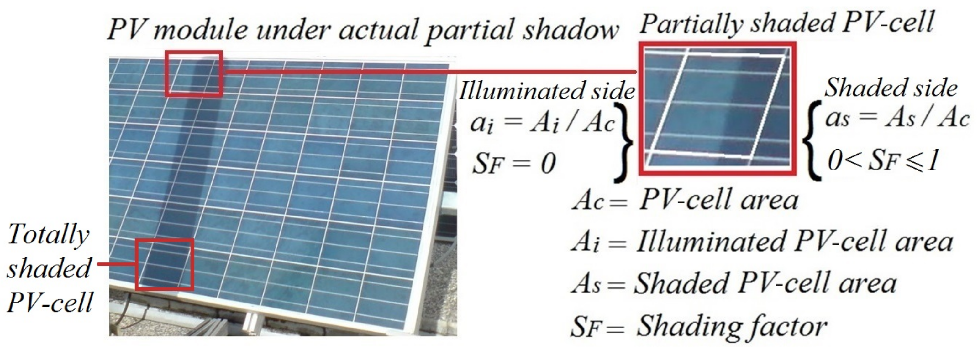
Figure 3 shows that, in a PV module, the partially shaded cells have two main shadow features. The first feature is the shadow geometry represented by $a_s+a_i=1,$ where $a_s$ is the fraction of shaded cell area and $a_i$ is the fraction of illuminated cell area. The second shadow feature includes the optical properties of the solar irradiance on the PV module represented by the shadow transmittance $\tau$ and the shading factor $S_f$. The shadow transmittance $\tau$ is defined by the ratio between the scattered irradiance $G_s$ on the shadow and the incident irradiance $G_i$, where $\tau =G_s/G_i$ [18]. $\tau =0$ means that all the available irradiance is blocked in the interest region. In contrast, $\tau =1$ means that all the available irradiance shines on the interest region because the scattered irradiance becomes $G_s=G_i$. The shading factor $S_f$ is defined in Equation (3) to describe the shadow opacity [36],

$$S_f=1-\frac{G_s}{G_i},$$

(3)

where $0\le S_f\le 1$. $S_f=0$ means that the available irradiance shines on the interest region. In contrast, $S_f=1$ means that all available irradiance is blocked in the interest region. Then, the relation between $\tau$ and $S_f$ is given by Equation (4):

$$S_f+\tau =1.$$

(4)

Figure 3. Partially shaded PV-cell.

Physical meaning of Equation (4) shows that the shadow parameters of shading factor $S_f$ and shadow transmittance $\tau$ are complementary. For instance, a totally shaded PV-cell ($a_s=1$) with a shading factor $S_f=0.8$ means that only the 20% of the available irradiance achieves the PV-cell surface, which represents a shadow transmittance $\tau =0.2$.

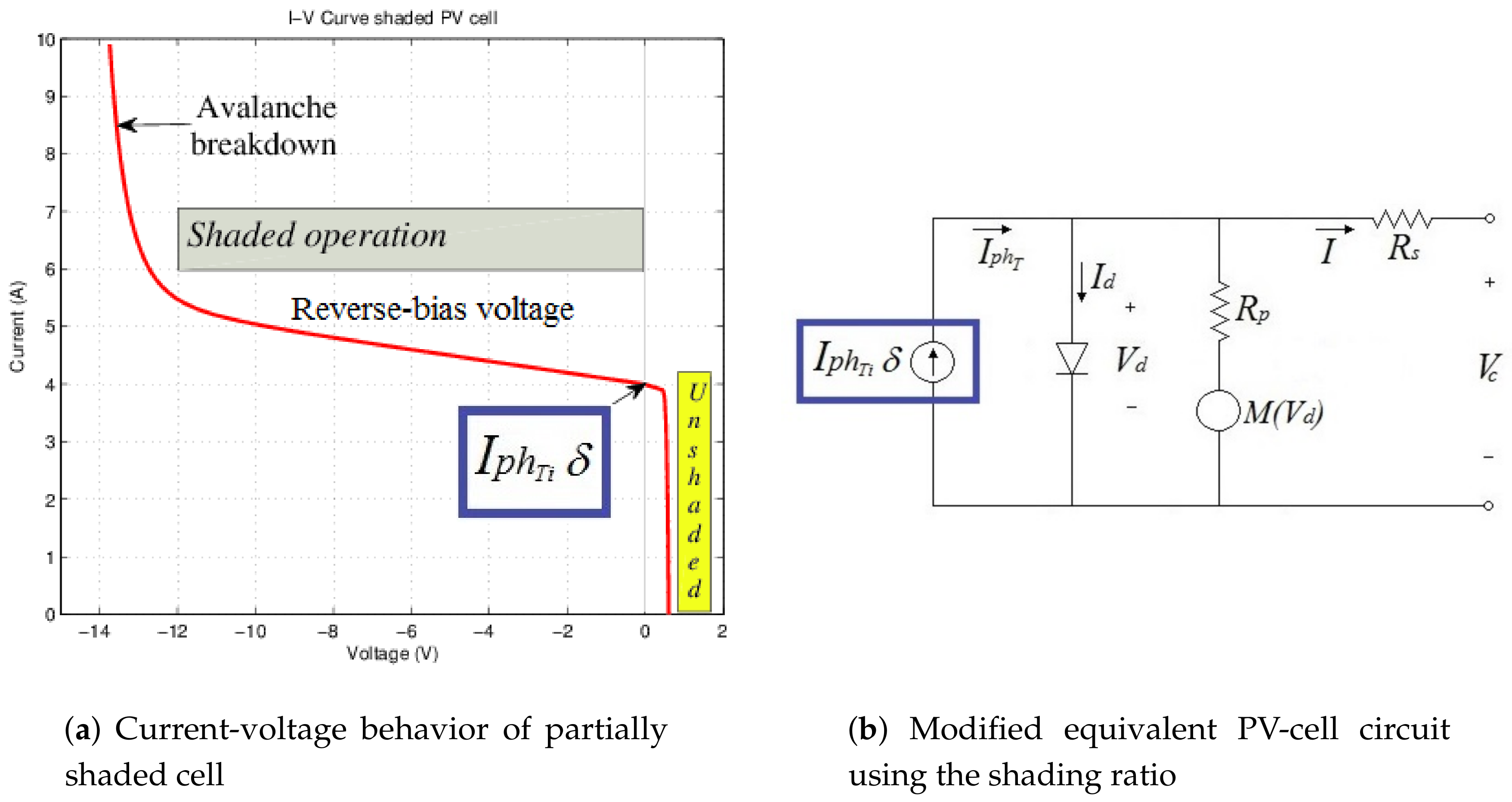
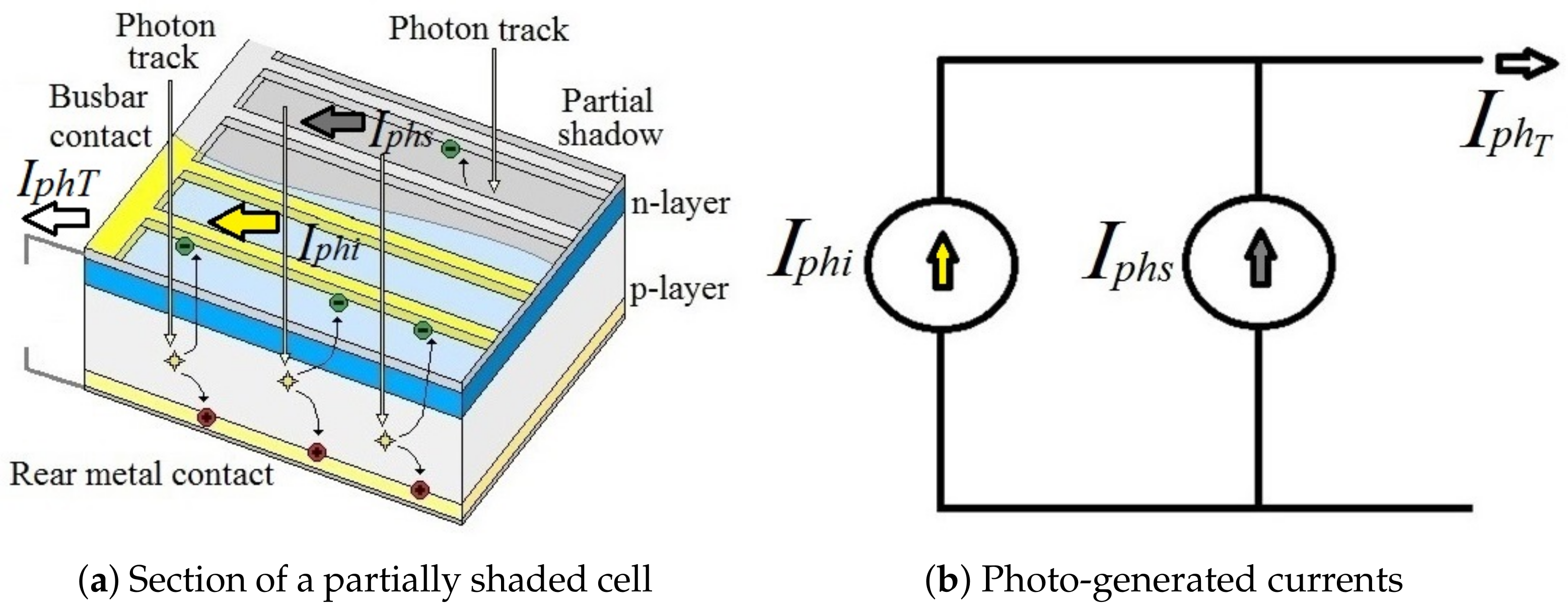
Figure 4a shows a 3D schematic section of a partially shaded PV-cell. In Figure 4, $I_{p{h}_i}$ and $I_{p{h}_s}$ represent the photo-generated currents in the illuminated and shaded areas. $I_{p{h}_T}$ defined as the total photo-generated current. As shown in Figure 4a, electron–hole pairs are generated when photons arrive at the p–n junction in the illuminated area. As a result, a photo-generated current $I_{p{h}_i}$ is produced in the illuminated area. In contrast, fewer photons can arrive to the p–n junction in the shaded area, which produces lower photo-generated current $I_{p{h}_s}$ in the shaded area. Therefore, using a simplified approach, the total photo-generated current $I_{p{h}_T}$ depends on contributions of shaded and unshaded areas, which is defined in Equation (5). Figure 4b shows the equivalent circuit for the photo-generated currents [28].

Figure 4. Photo-generated currents in a partially shaded PV-cell.

$$I_{p{h}_T}=I_{p{h}_i}+I_{p{h}_s}.$$

(5)

Using the current density definition $J=I/A$ for linking the electrical characteristics and the shadow geometric, we obtain Equation (6):

$$I_{p{h}_T}=J_{p{h}_i}{A}_i+J_{p{h}_s}{A}_s=J_{p{h}_i}{a}_i{A}_c+J_{p{h}_s}{a}_s{A}_c.$$

(6)

Considering the relation between the illuminated and shaded current densities given by the shadow transmittance, $J_{p{h}_s}=\tau J_{p{h}_i}$,

$$I_{p{h}_T}=J_{p{h}_i}{A}_c\left(a_i+\tau a_s\right),$$

(7)

as described previously $S_f+\tau =1$ and $a_s+a_i=1$. Thus,

$$I_{p{h}_T}=J_{p{h}_i}{A}_c\left(1-a_s{S}_f\right).$$

(8)

Given that $J_{p{h}_i}$ represents the photo-generated current produced per unit cell area in the illuminated side and $A_c$ defined as the total PV-cell area, the factor $J_{p{h}_i}{A}_c$ can be interpreted as the photo-generated current $I_{p{h}_{Ti}}$ that should be provided by the PV-cell in totally illuminated conditions . Therefore, Equation (7) can be rewritten as seen below:

$$I_{p{h}_T}=I_{p{h}_{Ti}}\left(1-a_s{S}_f\right).$$

(9)

The physical meaning of Equation (9) represents that the total photo-generated current $I_{p{h}_T}$ is proportional to the totally illuminated photo-generated current $I_{p{h}_{Ti}}$ given a ratio that depends on the shadow properties [28]. Equation (9) shows that the total photo-generated current depends on the shaded area percentage $a_s$ and the shadow opacity $S_f$ but is independent of the shadow shape. Defining this relation by the shading ratio $\delta$, Equation (10) is obtained:

$$\delta =1-a_s{S}_f.$$

(10)

Thus, the total photo-generated current $I_{p{h}_T}$ is given through Equation (11). In the $I_{p{h}_T}$ expression, the totally illuminated photo-generated current $I_{p{h}_{Ti}}$ is evaluated using Equation (12) and considering $G_i$ as the incident irradiance in totally unshaded conditions, which was clarified previously in Equation (2):

$$I_{p{h}_T}=I_{p{h}_{Ti}}\delta ,$$

(11)

$$I_{p{h}_{Ti}}=\left[I_{sc\_STC}+\left(C_{Ti}\left(T_c-T_{STC}\right)\right)\right]\frac{G_i}{G_{STC}}.$$

(12)

In addition, Equation (13) is defined by considering $I_{s{c}_{Ti}}$ as the totally illuminated short-circuit current for unshaded cell conditions:

$$I_{p{h}_{Ti}}\approx I_{s{c}_{Ti}}.$$

(13)

Thus,

$$I_{p{h}_T}\approx I_{s{c}_{Ti}}\delta .$$

(14)

We propose extending the model presented by Bishop [15] while using $I_{p{h}_T}$ for reformulating Equation (1) and Equation (15). At this point, it is important to highlight that the shading ratio $\delta$ depends on the quantifiable parameters $a_s$ and $S_f$ . Therefore, $\delta$ is also quantifiable. Figure 5a outlines the current–voltage behavior of a shaded PV-cell according to Equation (15). The equivalent PV-cell circuit is shown in Figure 5b. This simplified $\delta$ factor improves the description scope of shaded PV systems including measurable shadow features without needing to increase the computational effort.

Figure 5. Equivalent circuit and I–V curve of the partially shaded PV-cell.

$$I=\underset{I_{ph}}{\underbrace{I_{p{h}_{Ti}}\delta }}-I_0\left[e^{\left(\frac{V_c+I{R}_s}{V_t}\right)}-1\right]-\frac{V_c+I{R}_s}{R_p}\left[1+k{\left(1-\frac{V_c+I{R}_s}{V_b}\right)}^{-n}\right].$$

(15)

Equation (15) is a nonlinear equation that can be solved using numerical methods. The numerical method usually employed to solve these types of equations is the Newton–Raphson method [4]. The method starts with a function $f\left(V_c\right)$ defined as $f\left(V_c\right)=0$ as rewritten below in Equation (16):

$$f\left(V_c\right)=I_{p{h}_{Ti}}\delta -I-I_0\left[e^{\left(\frac{V_c+I{R}_s}{V_t}\right)}-1\right]-\frac{V_c+I{R}_s}{R_p}\left[1+k{\left(1-\frac{V_c+I{R}_s}{V_b}\right)}^{-n}\right].$$

(16)

Given that the function satisfies the condition $f^{\prime }\left(V_c\right)\ne 0$, the following iterative process is repeated until a sufficiently accurate value is reached:

$${V_c}_{n+1}={V_c}_n-\frac{f({V_c}_n)}{f^{\prime }({V_c}_n)}.$$

(17)

The solution of the iterative process in Equation (17) describes the PV-cell voltage given the influence of the shading ratio $\delta$ and a known I current. The solution of this iterative process is performed for a range of I currents from 0 to $I_{sc}$ and for the respective shading ratios $\delta$ of shaded PV cells. This method allows for calculating the voltage at the PV-cell level under several working conditions. Nevertheless, a series of connections of PV-cells form PV modules and it is required to go in depth about this aspect. The following section presents a systematic perspective to analyze the influence of the shading ratio on PV modules.

3.2. Influence of the Shading Ratio $\delta$ on the PV Module Behavior

This section relates the previous proposed approach with shadow patterns to extend the shadow impact analysis at the level of PV modules. Series connections of PV-cells form PV modules, and PV module manufacturing usually connects by-pass diodes to groups of PV-cells for decreasing the damage risk [29]. Thus, the voltage in a PV module $V_p$ with m groups of q PV-cells and by-pass diode voltage $V_{BD}$ is given by Equation (18):

$$V_p=\sum _{j=1}^m{V}_{G_j} where V_{G_j}=\left\{\begin{array}{c}{\sum }_{i=1}^q{V}_{c_i} if {\sum }_{i=1}^q{V}_{c_i}\ge 0,\hfill \\ V_{BD}\hspace{1em}if {\sum }_{i=1}^q{V}_{c_i}<0.\hfill \end{array}\right.$$

(18)

The PV-cell voltages $V_{c_i}$ come from the solution of the nonlinear Equation (16) by applying the numerical Newton–Raphson method of Equation (17). In addition, the parameters $I_0$, $R_s$, $V_t$, and $R_p$ of Equation (16) have been extracted according to the iterative methods presented in Ref. [5]. The parameters k and n of the multiplier factor proposed by Bishop in Ref. [15] have been extracted using nonlinear curve fitting methods from experimental results in shaded conditions with unconnected by-pass diodes. The parameter $V_b$ depends on the PV module technology and it has been fitted according to operation regions proposed in Ref. [29].

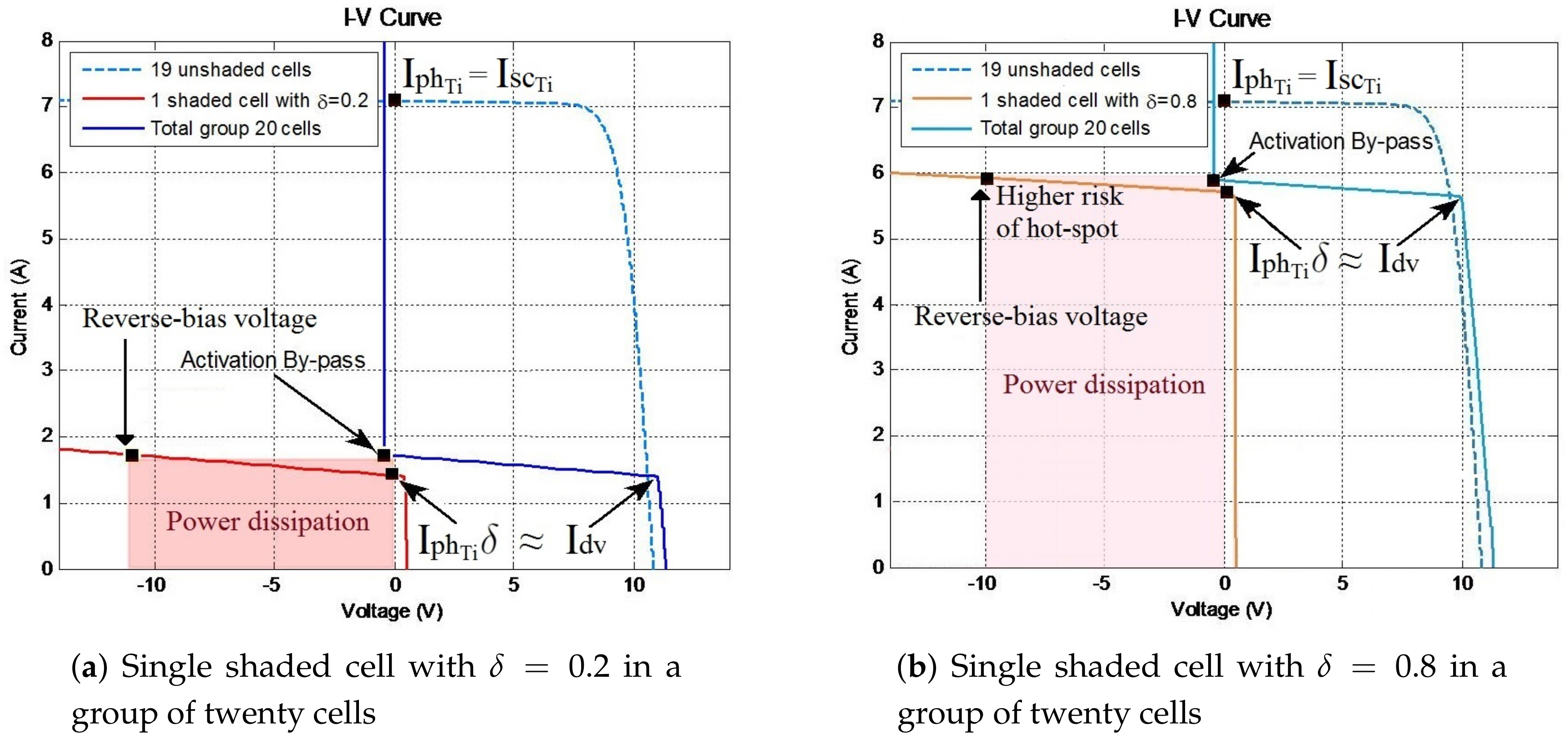
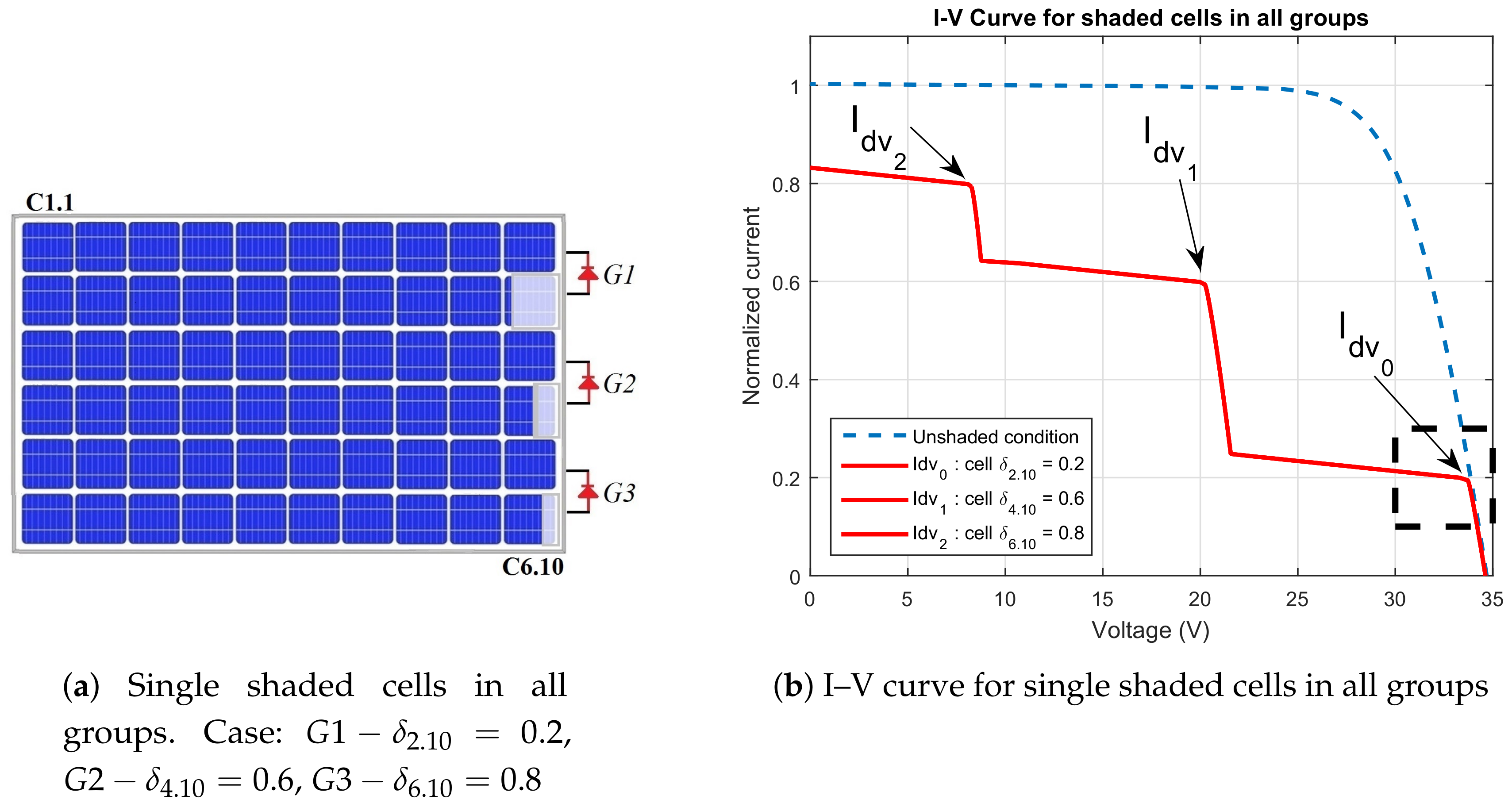
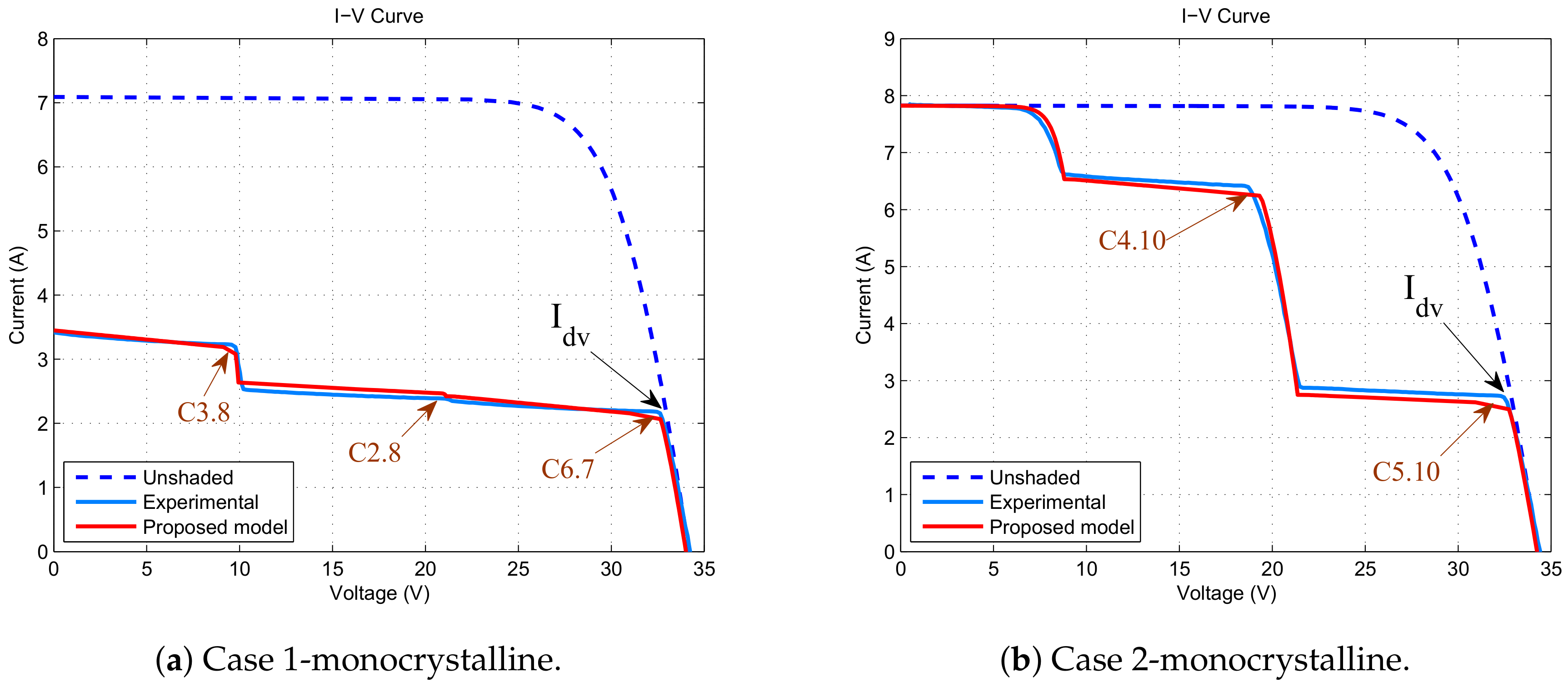
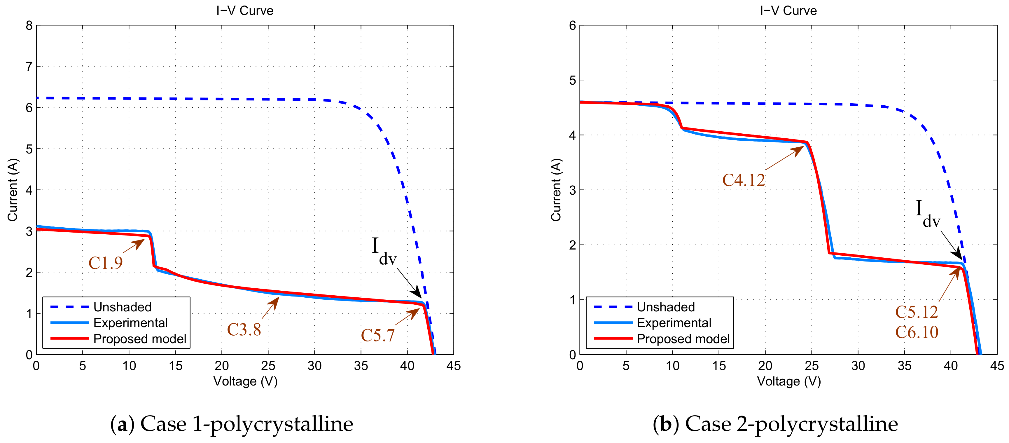
Solutions of Equations (15) and (18) for a group of twenty cells with a single shaded cell provides the results in Figure 6. As shown in Figure 6, a partial shadow in a single cell can change the normal behavior of the group drastically. Denoting $I_{dv}$ as the divergence current where the I–V curve diverges of normal operation in shaded conditions given by $\delta <1$, and the comparison of results in Figure 6a,b allows for deducing the behavior of $I_{dv}$ described by Equation (19):

$$I_{dv}\approx I_{p{h}_{Ti}}\delta \hspace{1em}\hspace{1em}for \delta <1.$$

(19)

Figure 6. Influence of $\delta$ in a group of twenty cells with a single shaded cell.

In addition, the totally illuminated short-circuit current was considered in Equation (13) as $I_{s{c}_{Ti}}\approx I_{p{h}_{Ti}}$. Then,

$$I_{dv}\approx I_{s{c}_{Ti}}\delta \hspace{1em}\hspace{1em}for \delta <1.$$

(20)

Equation (19) is deduced because the voltage in the shaded PV-cell begins to be negative when the PV-cell current is higher than $I_{p{h}_{Ti}}\delta$, which leads to a prominent change of the I–V curve. If the PV-cell current follows increasing, the PV-cell voltage is each time more negative until achieving the activation of the by-pass voltage. In this operation condition, the shaded PV-cell dissipates power due to the negative voltage and risk of damage can arise. 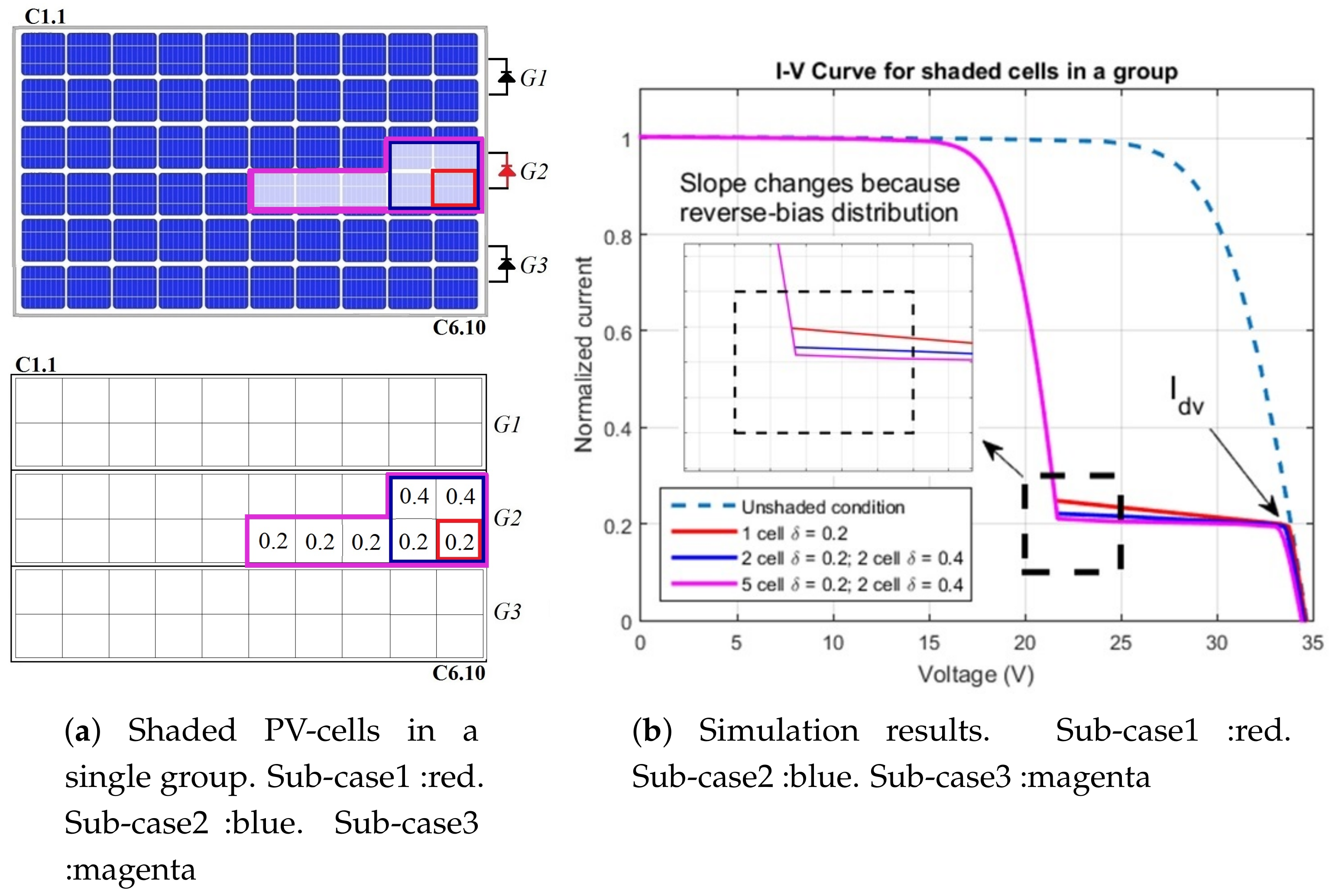Figure 6 shows that the situation can get worse if the shading ratio is higher because the dissipate power increases. This situation can induce hot-spots if the partial shadows are small and permanent. Failures of this type have been reported in literature and require preventive actions to avoid the deterioration of the PV system performance [37].

Figure 6 also allows for deducing the relation between the shaded PV-cells in a group with the lowest shading ratio. Assuming a case in which the shaded PV-cells of Figure 6a,b are in the same group, the lowest shading ratio of Figure 6a would lead the group toward the by-pass activation condition. Therefore, the shading ratio of the Figure 6b would have a minimum impact in the divergence current because the by-pass diode is already active. This operation principle can be extended to several shaded cells with different shading ratios because the lowest shading ratio is the first to activate the by-pass diode.

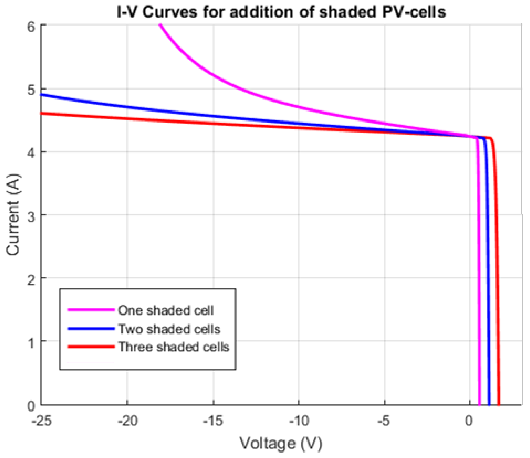
Figure 6 shows that the reverse-bias voltage is critical for the structural healthy of the PV-module. For that reason, in Figure 7, the I–V behavior is depicted in reverse-bias condition for several shaded cells. In this case, one PV-cell has a higher slope because the proximity of the breakdown voltage. In contrast, the illustrative example of Figure 7 shows that increasing the N shaded PV-cell multiplies the negative voltage N times because the PV-cell are connected in series. Therefore, the slope in the negative region decrease and for a given current interval $Slope=▵I/\left(N\ast ▵V\right)$.

Figure 7. Simulation of I–V Curves for addition of shaded PV-cells.

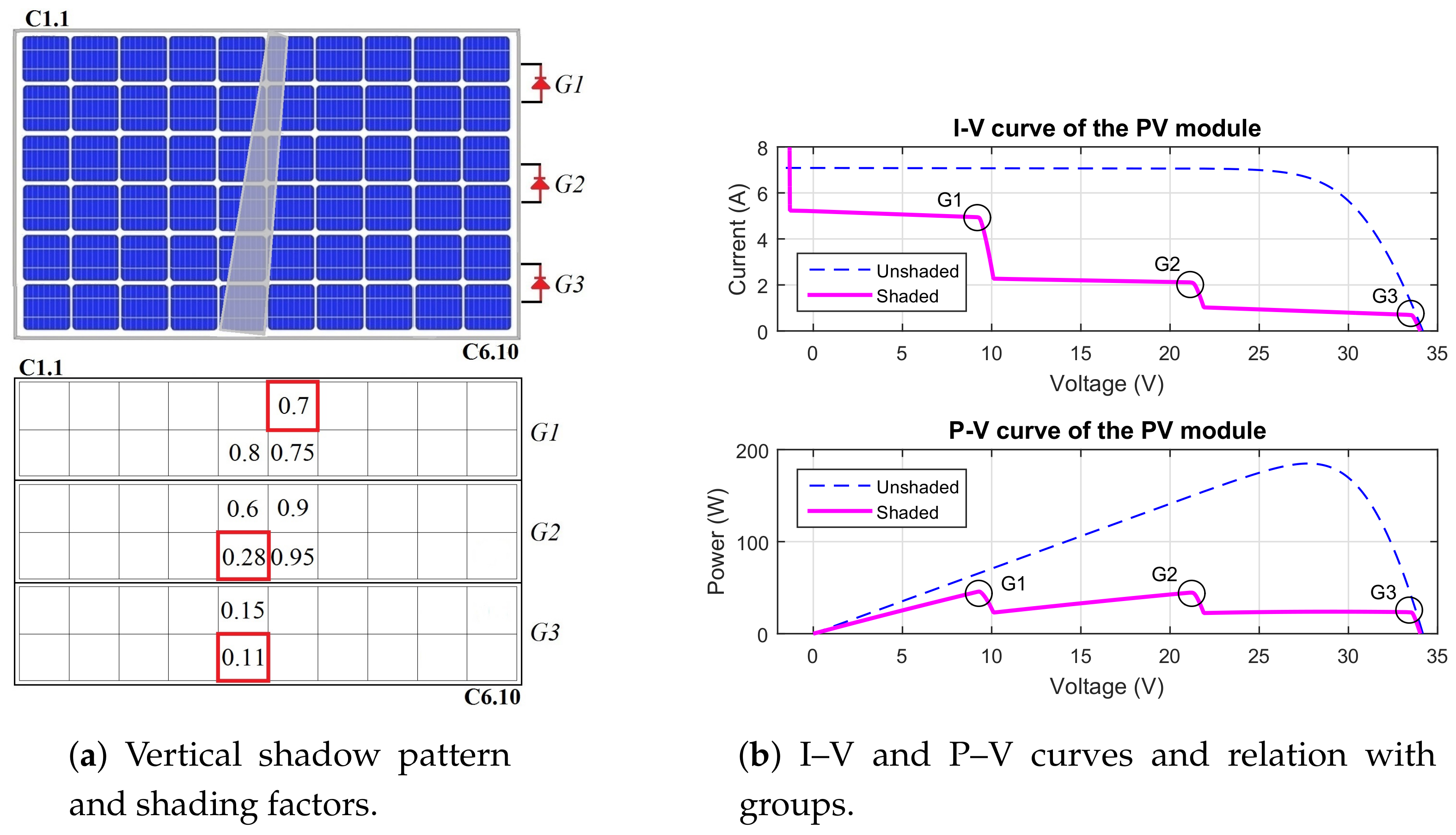
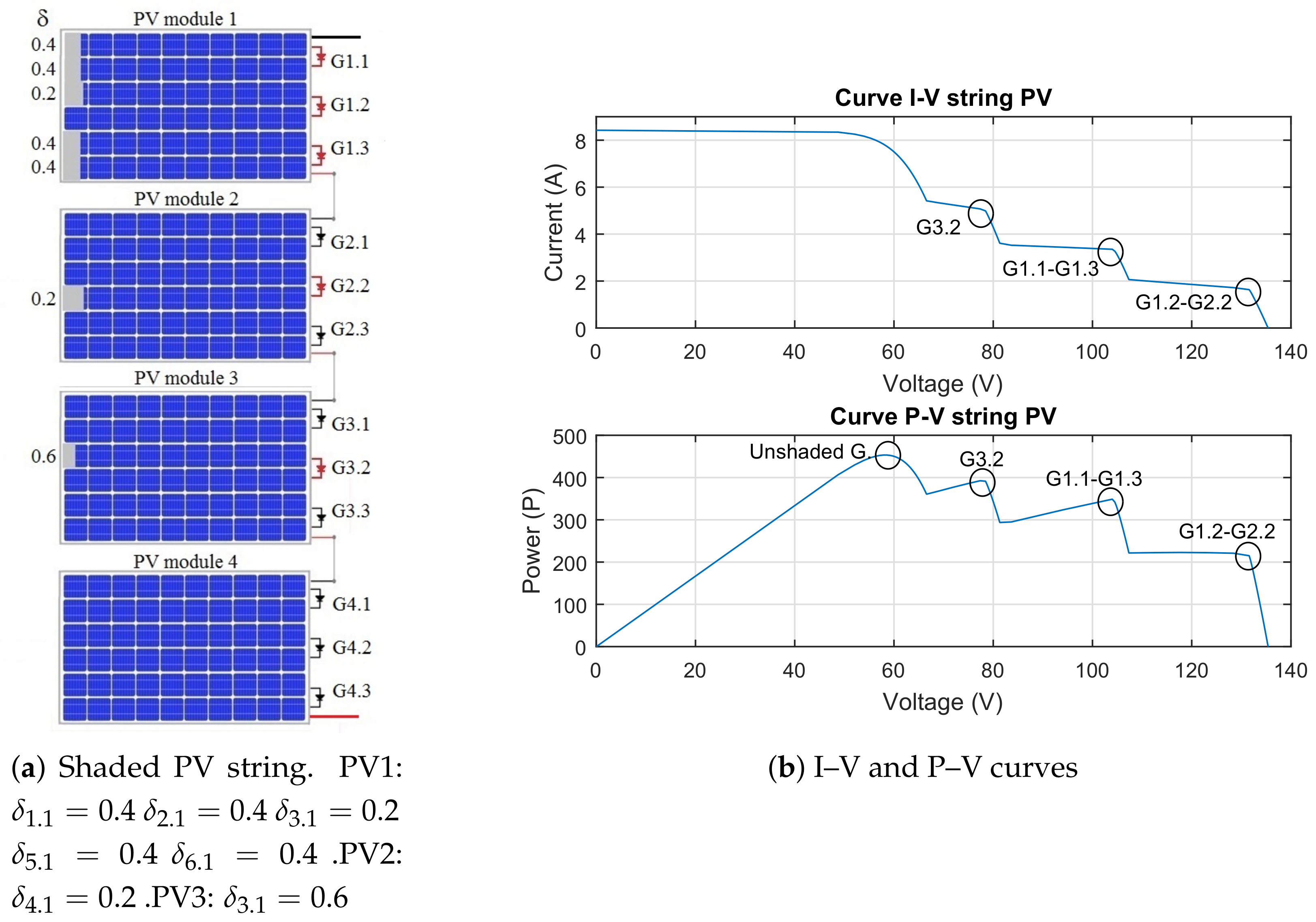
Figure 8 extends the analysis to several shaded PV cells in a PV module. These figures show the interrelation between the divergence currents and the maximum power points (MPPs). As shown in Figure 8, z represents the index for the lowest shading ratios ${\delta }_z$ in each group where $z=\left\{0,1,2,‥,g-1\right\}$ and g is the total number of groups connected in series. $V_{mz}$ and $I_{mz}$ are the voltages and currents at the MPPs. The relation between the MPPs and the lowest shading ratios ${\delta }_z$ is given by the behavior of the divergence currents $I_{dvz}$ and the local MPPs. Figure 8 allows for deducing that $I_{dvz}\approx I_{mz}$ because the MPPs arise around the current divergence. Nevertheless, an exception to this pattern is presented in unshaded groups where $I_{mz}\approx I_{mp}$.

Figure 8. I–V and P–V curves for a partially shaded PV module.

$▵V_z$ is defined in Equation (21) as a proportional relation between the voltage difference $V_{oc}-V_{mp}$ and the corresponding shading ratio ${\delta }_z$ for the shading ratios arranged from the lower to the higher ${\delta }_z<{\delta }_{z+1}$. The physical meaning of Equation (21) represents that the voltage displacement of $V_{mz}$ in relation to the local MPPs in an unshaded condition is associated with the shading ratio ${\delta }_z$.

$$▵V_z\approx \left(V_{oc}-V_{mp}\right){\delta }_z\hspace{1em}for z=\left\{0,1,\dots ,g-1\right\}, g=number of groups, and {\delta }_z<{\delta }_{z+1}.$$

(21)

All groups are connected in series and each group proportionally contributes to the open circuit voltage $V_{oc}$. For this reason, the voltage $V_{mz}$ at the local MPPs is expressed as a fraction of $V_{oc}$ and $▵V_z$. For the illustrative example of the Figure 8, the expressions for the voltages $V_{mz}$ at the local MPPs are given from Equation (22) to Equation (24), where $V_{BD}$ is the forward by-pass diode voltage which displaces the proportion of $V_{oc}$:

$$V_{m0}=V_{oc}-▵V_0,$$

(22)

$$V_{m1}=\left(\frac{2}{3}{V}_{oc}\right)-\left(\frac{2}{3}▵V_1\right)-V_{BD},$$

(23)

$$V_{m2}=\left(\frac{1}{3}{V}_{oc}\right)-\left(\frac{1}{3}▵V_2\right)-2V_{BD}.$$

(24)

A general expression of $V_{mz}$ is deduced in Equation (25) for g groups and $z=\left\{0,1,\dots ,g-1\right\}$,

$$V_{mz}=\left(\frac{g-z}{g}\right)V_{oc}-\left(\frac{g-z}{g}\right)▵V_z-\left(z{V}_{BD}\right).$$

(25)

For ${\delta }_z<1$ and ${\delta }_z<{\delta }_{z+1}$,

$$P_{mz}=V_{mz}{I}_{mz}\approx V_{mz}{I}_{dvz}\approx V_{mz}{I}_{s{c}_{Ti}}{\delta }_z,$$

(26)

$$P_{mz}\approx \left[\left(\left(\frac{g-z}{g}\right)\left(V_{oc}-▵V_z\right)\right)-\left(z{V}_{BD}\right)\right]I_{s{c}_{Ti}}{\delta }_z.$$

(27)

For unshaded groups ${\delta }_z=1$ and $P_{mz}$ is given by Equation (28),

$$P_{mz}=V_{mz}{I}_{mp},$$

(28)

$$P_{mz}\approx \left[\left(\left(\frac{g-z}{g}\right)V_{mp}\right)-\left(z{V}_{BD}\right)\right]I_{mp}.$$

(29)

Equations (27) and (29) allow a fast approximation to the MPPs for known shadow patterns and unshaded operation parameters. The procedure to evaluate the MPPs is described as follows:

Step 1:

Determination of the lowest shading ratios ${\delta }_z$ in each group, arrangement of shading ratios from the lower to the higher ${\delta }_z<{\delta }_{z+1}$.

Step 2:

Evaluation of $V_{mp}$, $I_{mp}$, $I_{s{c}_{Ti}}$, and $V_{oc}$ from unshaded condition, considering $V_{BD}\approx 0.7V$.

Step 3:

Calculation of $P_{mz}$ for $z=\left\{0,1,\dots ,g-1\right\}$ using Equation (27) if ${\delta }_z<1$ or Equation (29) if ${\delta }_z=1$.

Step 4:

In the special case of ${\delta }_z={\delta }_{z+1}$, the sequence of values for $P_{mz}$ and $P_{mz+1}$ are evaluated normally. However, only the highest value of power defines the region for the local MPP.

Given the proposed modeling approach through this section, the next stage will analyze the simulation of shaded PV modules.

4. Simulation Analysis of Shaded PV Modules

The cases of shadow patterns in this section have been selected to illustrate the potential features of proposed approaches in simulation. First, two cases describe the impact of single shaded cells scattered in several groups and the impact of shaded cells grouped in a single group. Then, two cases are intended to show the shadow movement impact. The final simulation targets a shaded PV string.

The simulations have been performed in a conventional computational platform by solving Equations (16)–(18) according to the lineaments presented in Section 3. In addition, the simulated shading ratios $\delta$ are set for analysis and further correlation with experimental patterns. The shaded PV-module images in this section have only a character illustrative and do not represent any software in particular.

4.1. Simulation of Partially Shaded PV Modules

The nominal parameters of the simulated PV modules are $I_{sc}=8.3$ A and $V_{oc}=37.3$ V with simulation conditions of incident irradiance $G_i=850$ W/m${}^2$ and cell temperature $T_c=45 {}^{\circ }$C. The cases consider a uniform shading factor $S_f=0.8$. We also consider a conventional PV module with sixty cells distributed in groups of twenty cells connected to by-pass diodes [3]. The analysis uses a matrix notation $ij$ where ${\delta }_{ij}$ represents the shading ratio of a PV-cell in the relative position $ij$ in a PV module.

The first case depicted in Figure 9 shows all groups with a single shaded cell. This simulation is intended to study the impact of single shaded cells in the normal current–voltage behavior. In Figure 9, the PV module current $I_{PV}$ is normalized in ratio to $I_{s{c}_{Ti}}=7.1$ A. Therefore, on the y-axis, the $I_{Norm}=I_{PV}/I_{s{c}_{Ti}}$. This simulation case shows that the lowest divergence current $I_{dv}$ is proportional to the shaded cells with the lowest value of $\delta$. For instance, the first divergence current $I_{d{v}_0}$ in Figure 9b is caused by the PV-cell with ${\delta }_{2.10}=0.20$ of group one. Figure 9 confirms that the divergence current $I_{dvz}$ due to each group is close to $I_{dvz}={\delta }_z{I}_{s{c}_{Ti}}$, where ${\delta }_z$ depends on the shaded cell $C_{ij}$ with the lowest value of $\delta$ in the group.

Figure 9. Study case of shadow pattern for single shaded cells in all groups.

Figure 10 depicts three sub-cases of distributed shaded cells in a single group. As shown in Figure 10a, the first sub-case has one shaded cell with $\delta =0.2$. The second sub-case has two shaded cells with $\delta =0.2$ and the other two cells with $\delta =0.4$. The third sub-case has five cells with $\delta =0.2$ and the other two cells with $\delta =0.4$. The simulation results show that the lowest value of $\delta$ in a group with several shaded cells causes the divergence current $I_{dv}$. In addition, Figure 10b illustrates that a greater number of shaded cells in a group causes a decrease in the I–V curve slope. This phenomenon is due to the behavior of the shaded cells in the reverse-bias as described previously. As a result, a single shaded cell in a group has a higher I–V curve slope and more risk of hot-spots than a group with several shaded cells because the reverse-bias voltage and power dissipation distribution [2,3].

Figure 10. Representation of three sub-study cases with shadow patterns distributed in a single group.

Figure 9 and Figure 10 allowed for the analysis of single shaded PV cells and single shaded groups. However, the shadow displacement in daily conditions can generate several irregular shadow patterns. To describe this more realistic aspect, Figure 11 and Figure 12 illustrate two irregular shadow patterns from a hypothetical pole, antenna, or chimney.

Figure 11. I–V and P–V behavior for diagonal shadow pattern in a PV module.

Figure 12. I–V and P–V behavior of the vertical shadow pattern in a PV module.

Figure 11a shows a diagonal shadow pattern and the associated shading ratios. In this case, Figure 11b shows that the group three with ${\delta }_{6.9}={\delta }_{5.10}=0.28$ produces the lowest divergence current $I_{d{v}_0}=0.28I_{s{c}_{Ti}}\approx 2A$, and the group two with ${\delta }_{4.10}=0.7$ produces the divergence current $I_{d{v}_1}=0.7I_{s{c}_{Ti}}\approx 5A$. After finding $I_{d{v}_0}$ and $I_{d{v}_1}$, the maximum power points (MPPs) are calculated using Equations (27) and (29) as described in Section 3.2. Table 1 lists these approximate and simulated MPPs. The results in Table 1 show a suitable agreement between actual and estimated MPPs. This simplified method allows for quickly identifying the global MPP and its source.

Table 1. Maximum power points—Case: diagonal shadow.

Parameter	Values
z	0	1	2
${\delta }_z$	0.28	0.7	1.0
Group	G3	G2	G1
$P_{mz}approx.$(W)	64.09	95.02	53.65
$P_{mz}simul.$(W)	68.06	98.39	55.27
$Rel.error$	0.06	0.03	0.03

Figure 12a describes a pattern in all vertical groups. This figure shows that the divergence currents depend on the lowest $\delta$ in each group. In addition, the other shaded cells impact the slope of the I–V curve without relevant contribution to the $I_{dv}$. Table 2 shows the simplified calculation of the approximate MPPs using Equations (27) and (29) of Section 3.2. These results show that the group G1 provides the global MPPs, which agrees with the simulation results. Therefore, Table 1 and Table 2 confirm that the MPPs can be localized from the lowest $\delta$ in each group and the parameters of unshaded operation without an exhaustive calculation from all of the shaded PV cells.

Table 2. Maximum power points—Case: vertical shadow.

Parameter	Values
z	0	1	2
${\delta }_z$	0.11	0.28	0.7
Group	G3	G2	G1
$P_{mz}approx.$(W)	26.02	41.54	43.05
$P_{mz}simul.$(W)	24.07	44.53	45.72
$Rel.error$	0.081	0.067	0.058

4.2. Simulation of Partially Shaded PV String

Figure 13 depicts the final studied case at level of PV string. To facilitate understanding, this figure highlights the most significant shaded PV cells in an irregular shadow pattern. The simulations results allow identifying four regions. The region $R_1$ depends on $G1.2$ and $G2.2$. In this region, PV1 ${\delta }_{3.1}$ and PV2 ${\delta }_{4.1}$ cause the lowest $I_{dv0}$ in the PV string. $R_1$ is extended by around 20V because the bypass activation of two groups. $G1.1$ and $G1.3$ produce region $R_2$. The divergence current $I_{dv1}$ in $R_2$ is proportional to the 40% of $I_{s{c}_{Ti}}$, which is caused by PV1 ${\delta }_{1.1}={\delta }_{2.1}={\delta }_{5.1}={\delta }_{6.1}=0.4$. Region $R_3$ is produced by $G3.2$ with the single PV-cell PV3 ${\delta }_{3.1}=0.6$. The bypass activation point and the I–V curve slope are higher in region $R_3$; therefore, this single cell is more vulnerable to dissipating power and generating hot-spots (see Figure 6b). Finally, $R_4$ depends on the unshaded PV groups and provides the highest MPP of all regions.

Figure 13. I–V and P–V curves of a shaded PV string.

Table 3 lists the MPPs for the studied PV string. These results illustrate a special case of Equations (27) and (29) to evaluate the approximate MPPs where equal ${\delta }_z$ appear in different groups. For this case, the sequence of values in Equations (27) and (29) are evaluated normally; however, only the highest MPP of equal ${\delta }_z$ is taken into account to define the MPP region and the global MPP. Finally, the results in Figure 13 and Table 3 confirm that this simplified methodology provides a suitable approximation to the MPPs at the level of PV strings. The next section summarizes the main identified findings.

Table 3. Maximum power points—Case: shaded string.

Parameter	Values
z	0	1	2	3	4	5
${\delta }_z$	0.2	0.2	0.4	0.4	0.6	1.0
Group	G1.2	G2.2	G1.1	G1.3	G3.2	Unsh.G.
$P_{mz}approx.$(W)	216.1	197.1	340.5	304.2	382.5	464.2
$P_{mz}simul.$(W)	220.9	-	348.8	-	391.30	453.2
$Rel.error$	0.022	-	0.024	-	0.023	0.024

4.3. Identified Patterns between the Shading Ratio and the PV Module Behavior

The following findings highlight the patterns identified from the interaction between the shading ratio and the partial shadows.

• The divergence currents $I_{dvz}$ are proportional to the lowest shading ratio ${\delta }_z$ in each shaded PV group. Thus, $I_{dvz}\approx {\delta }_z{I}_{s{c}_{Ti}}$ for ${\delta }_z<1$.
• Shaded cells have a minimal impact on the I–V curve if their shading ratio is greater than the lowest shading ratio in the same group.
• In a group, shaded cells with shading ratios close to the lowest shading ratio have a lower overheating risk because the reverse bias voltage is distributed between them.
• A single shaded cell in a group with higher shading ratio has a greater probability of being a hot-spot because of the power dissipation despite the by-pass diodes.
• The MPPs can be quickly identified from the lowest shading ratio in each group and the parameters for unshaded conditions.
• The above-mentioned patterns can be extended at the level of PV strings.

The next section presents the experimental tests to validate the proposed approach correlating the current voltage-behavior with shadow image patterns.

5. Experimental Validation and Discussion

This section describes the experimental setup for validating the analysis proposed in Section 3. In addition, this section outlines an experimental procedure to quantify the shading ratio using image processing methods. Experimental results are discussed.

5.1. Test for Partially Shaded PV Modules

The developed experiments consider two shadow cases as depicted in Figure 14 and Figure 15. Furthermore, the tests use monocrystalline and polycrystalline PV modules to compare these common commercial technologies. The PV module characteristics are listed in Table 4.

Figure 14. Experimental tests for monocrystalline PV module.

Figure 15. Experimental tests for polycrystalline PV module.

Table 4. Photovoltaic modules under testing.

Type Ref.	Monocrystalline Tenesol TE 2200	Polycrystalline Yingli solar YL290p-35b
Electrical parameters at STC
Maximum Power ($P_{mp}$)	250 Wp	290 Wp
Voltage at $P_{mp}$ ($V_{mp}$)	30.3 V	35.8 V
Current at $P_{mp}$ ($I_{mp}$)	8.3 A	8.1 A
Open circuit voltage ($V_{oc}$)	37.3 V	45.3 V
Short-circuit current ($I_{sc}$)	8.6 A	8.62 A

Figure 16a depicts the experimental setup performed in the platform ADREAM of the Laboratory for Analysis and Architecture of Systems (LAAS-CNRS) in Toulouse, France (43${}^{\circ }$33${}^{\prime }{44.3}^{″}$N 1${}^{\circ }$28${}^{\prime }{38.3}^{″}$E). In this setup, an I–V curve tracer (model MP-160, EKO Instruments, Tokyo, Japan) is used to detect the current–voltage signals. Furthermore, a pyrometer (model SP-Lite, Kipp&Zonen, Delft, the Netherlands) monitors the solar irradiance and a thermographic camera periodically measures the PV module temperature.

Figure 16. Experimental setup for model validation and image processing.

Simultaneously, a digital camera records the shadow pattern, which is shown in Figure 16b. The analysis of the shaded PV-cell areas is performed using image processing methods after contour selection. The selected image is converted from gray-scale image to a binary image through digital processing based on the histogram and Otsu’s method [38]. Finally, the shaded area is calculated using Equation (30) where $p_b$ is the total number of black pixels and $p_w$ is the total number of white pixels:

$$a_s=\frac{p_b}{p_b+p_w}.$$

(30)

The experimental test is described as follows:

Step 1:

Simultaneous measurements and recording of I–V curves, solar irradiance, PV module temperature, and shadow patterns.

Step 2:

Selection of synchronized I–V curves and image shadow patterns for analysis.

Step 3:

Image processing for measurement of shaded PV-cell areas in selected shadow patterns.

Step 4:

Shading ratio calculation for the PV-cell with the largest shaded area $a_{sL}$ using Equation (31). $I_{p{h}_{Ti}}$ is calculated using Equation (12). $I_{d{v}_L}$ is the first divergence-current point in the experimental I–V curve.

Step 5:

Calculate the shading factor $S_f$ for the PV-cell with the largest shaded area ${\delta }_L$ using Equation (32). In this experimental setup, the shading factor is considered uniform on the shaded cell because the I–V curve measurements and the shaded PV module image recording are synchronized.

Step 6:

Evaluate the shading ratio ${\delta }_{ij}$ for each shaded PV-cell.

Step 7:

The calculated shading ratios are used to evaluate the I–V and P–V characteristics of the PV modules:

$${\delta }_L=\frac{I_{d{v}_L}}{I_{p{h}_{Ti}}},$$

(31)

$$S_f=\frac{1-{\delta }_L}{a_{sL}}.$$

(32)

Table 5 summarizes the parameters and values for calculating the shading factor. The shading ratios ${\delta }_{ij}$ are calculated for each shaded PV-cell while considering their shaded area $a_{ij}$ and the same shading factor $S_f$. Table 6 and Table 7 list the shaded cell areas $a_{ij}$ obtained after image processing and the calculated shading ratios ${\delta }_{ij}$. These shading ratios are used to evaluate the I–V and P–V characteristics for the PV modules. Table 8 and Table 9 summarize the MPPs. Lastly, the experimental and calculated I–V curves are depicted in Figure 17 and Figure 18.

Table 5. Shading factor results for the PV modules under testing.

Type	Monocrystalline		Polycristalline
	Case 1	Case 2	Case 1	Case 2
$G_i$	820 W/m${}^2$	910 W/m${}^2$	710 W/m${}^2$	540 W/m${}^2$
$T_c$	31 ${}^{\circ }$C	31 ${}^{\circ }$C	31 ${}^{\circ }$C	30 ${}^{\circ }$C
$I_{p{h}_{Ti}}$	7.07 A	7.85 A	6.14 A	4.67 A
$I_{d{v}_L}$	2.16 A	2.7 A	1.33 A	1.66 A
$a_{sL}$	0.98	0.91	0.97	0.90
${\delta }_L$	0.31	0.34	0.22	0.36
$S_f$	0.70	0.72	0.8	0.71

Table 6. Shaded area and shading ratio for monocrystalline PV module Tenesol TE-2200.

	Case 1			Case 2
Group	${\mathit{C}}_{\mathit{ij}}$	${\mathit{a}}_{\mathit{ij}}$	${\mathit{\delta }}_{\mathit{ij}}$	${\mathit{C}}_{\mathit{ij}}$	${\mathit{a}}_{\mathit{ij}}$	${\mathit{\delta }}_{\mathit{ij}}$
1	C1.8	0.94	0.34
	C2.8	0.96	0.33
2	C3.7	0.17	0.88	C4.10	0.25	0.82
	C3.8	0.80	0.44
	C4.7	0.40	0.72
	C4.8	0.50	0.65
3	C5.7	0.80	0.44	C5.9	0.35	0.75
	C5.8	0.20	0.86	C5.10	0.91	0.34
	C6.7	0.98	0.31	C6.8	0.40	0.72
				C6.9	0.89	0.37
				C6.10	0.15	0.89

Table 7. Shaded area and shading ratio for polycrystalline PV module YL290p-35b.

	Case 1			Case 2
Group	${\mathit{C}}_{\mathit{ij}}$	${\mathit{a}}_{\mathit{ij}}$	${\mathit{\delta }}_{\mathit{ij}}$	${\mathit{C}}_{\mathit{ij}}$	${\mathit{a}}_{\mathit{ij}}$	${\mathit{\delta }}_{\mathit{ij}}$
1	C1.9	0.68	0.46
	C2.8	0.64	0.49
	C2.9	0.66	0.47
2	C3.8	0.96	0.23	C4.12	0.19	0.86
	C3.9	0.11	0.91
	C4.7	0.65	0.48
	C4.8	0.65	0.48
3	C5.6	0.10	0.92	C5.10	0.21	0.85
	C5.7	0.97	0.22	C5.11	0.80	0.43
	C5.8	0.11	0.91	C5.12	0.90	0.36
	C6.6	0.65	0.48	C6.8	0.22	0.84
	C6.7	0.65	0.48	C6.9	0.78	0.45
				C6.10	0.90	0.36
				C6.11	0.37	0.74

Table 8. Maximum power points—Monocrystalline.

Parameter	Case 1			Case 2
z	0	1	2	0	1	2
${\delta }_z$	0.31	0.33	0.44	0.34	0.82	1.0
Group	G3	G1	G2	G3	G2	G1
$P_{mz}approx.$(W)	70.3	48.3	28.7	85.5	120.3	59.2
$P_{mz}exper.$(W)	70.2	51.6	31.1	88.2	119.4	60.2
$Rel.error$	0.001	0.064	0.078	0.031	0.008	0.017

Table 9. Maximum power points—Polycrystalline.

Parameter	Case 1			Case 2
z	0	1	2	0	1	2
${\delta }_z$	0.22	0.23	0.46	0.36	0.86	1.0
Group	G3	G2	G1	G3	G2	G1
$P_{mz}approx.$(W)	55.5	37.8	33.4	68.4	93.8	44.9
$P_{mz}exper.$(W)	55.2	42.1	36.9	67.8	94.9	45.7
$Rel.error$	0.006	0.103	0.094	0.01	0.01	0.02

Figure 17. I–V curves for test with monocrystalline PV module.

Figure 18. I–V curves for tests with polycrystalline PV module.

5.2. Discussion of Results

The experimental results confirm the correlation between the shading ratio $\delta$ and the I–V curve. For instance, Table 6 and Figure 17 experimentally show that the first divergence points in the I–V curves are caused by the lowest shading ratios of PV-cells C6.7 and C5.10. Additionally, Table 7 and Figure 18 allow for validating this interpretation.

Considering a uniform $S_f$, the results also demonstrate that the smaller shaded cell areas in comparison with the larger shaded cell areas in the same group provide a minimal contribution to the I–V curve. For instance, the PV-cells C3.7 and C5.8 of case 1-monocrystalline (Table 6) have a minimal impact on the I–V characteristics of Figure 17a. In contrast, shaded cells with small shaded areas are able to modify the I–V curve if they have the lowest shaded area in the group. For example, the PV-cell C4.12 in Case 2-polycrystalline is able to cause changes in the I–V curve of Figure 18b.

Figure 18a,b show that shaded PV-cells in a group, with shading ratios near to the lowest shading coefficient in the group, produce I–V curves with lower slopes because the behavior of the reverse-bias voltage. For instance, PV-cells C5.12 and C6.10 of Case 2-polycrystalline cause a lower slope than caused by the PV-cell C4.12 in Case 2-polycrystalline. Therefore, PV-cell C4.12 has more risk of dissipating power. Table 10 lists the slopes for the case 2-monocrystalline and the case 2-polycrystalline, which have a single shaded cell in a group. Results in Table 10 show a slight difference in the case of monocrystalline but a more significant difference in the case of polycrystalline. Authors also have addressed a detailed experimental study about the partial shading and the slope identification, which has been reported in Ref. [3]:

$$MSE=\frac{1}{n}\sum _{i=1}^n{\left(e_i\right)}^2.$$

(33)

Table 10. Slopes of I–V curves.

Region	Monocryst. Case 2	Region	Polycryst. Case 2
8 V–18 V	37 mA/V	12 V–24 V	20.37 mA/V
22 V–32 V	33.8 mA/V	28 V–42 V	11.11 mA/V

We use the mean square error (MSE) to assess the modeling accuracy based on the shading ratio. The MSE values listed in Table 11 illustrate the model accuracy for the experimental and simulated I–V curves depicted in Figure 17 and Figure 18. Table 11 shows that the proposed approach is suitable for describing the current–voltage behavior of partially shaded PV modules in both monocrystalline and polycrystalline technologies. However, the behavior of polycrystalline modules slightly varies from monocrystalline modules because of the lower breakdown voltage in polycrystalline technology [29]. This phenomenon is more appreciable in the region from 13 V to 40 V of Figure 18a, which can lead to higher risk of hot-spots [29].

Table 11. Mean squared error (MSE) from simulated and experimental I–V curves for model validation.

	Monocrystalline		Polycrystalline
Error calculation	Case 1	Case 2	Case 1	Case 2
MSE	0.92	1.07	0.89	1.01

The MSE of model validation in Table 11 also shows a slightly difference for case 1 and case 2 in both technologies. This difference can be produced by several factors such as changes in the internal parameters, current path, or leakage currents. Indeed, some authors have shown that series and shunt resistances are affected by the irradiance conditions [21]. Soto et al. suggest that the series resistance depends on the irradiance level because its value decreases for lower irradiance and even can suffer negative values [39]. Earlier works also indicate negative values for the series resistance under low irradiance [40]. In Ref. [21], the series resistance increases at the same time as the shadow rate, which increases the amount of power dissipated by the series resistance. Nevertheless, most authors consider these variations less relevant by treating the series resistance independent of the incident irradiance and temperature and obtaining sufficient accuracy [41,42]. In contrast, the study of the low irradiance conditions on the shunt resistances have been more widespread in literature because of the strong impact of the reverse-bias conditions [43,44].

For the local maximum power points (MPPs), the results from Table 6 to Table 9 show the integration of image processing methods with the proposed modeling for fast localization of the global MPP. The approximate MPPs for monocrystalline and polycrystalline cases are calculated using Equations (27) and (29), and results are registered in Table 8 and Table 9. Indeed, these results highlight the correlation between the lowest shading ratios and the MPP calculation. These characteristics of simplified and fast localization of MPPs are potentially applicable to current supervision methods of power production based on image recognition [13,14].

Finally, the proposed methodology through this section can contribute to the supervision strategies based on image processing by considering the following findings in terms of shaded areas:

• Shaded cells with the highest shaded area in each group cause the divergence currents.
• Several shaded cells in a single PV group negligibly modify the operation point imposed by the PV-cell with the highest shaded area.
• Localized shadows on single shaded cells in a group are more harmful because overheating can arise.
• Uniform shadows on several cells of the same group cause less structural risks.
• The MPPs can be quickly localized considering the shaded PV-cells with the highest shaded areas in each group.

5.3. Comparison with Other Approaches

In this section, the contributions presented through this paper are compared with the existing schemes in literature. Methodologies in Table 12 address the PV modeling concerns using different perspectives. Ref. [15] describes the reverse-bias behavior using a nonlinear multiplication factor associated with the shunt resistance current. However, the impact of partial shadows is not discussed. The second approach proposes a discrete method to ensure convergence [20]. This paper presents a generalized method mainly based on the Bishop modeling to simulate the electrical behavior of PV installations by discretizing currents and voltages in PV systems. In contrast, quantification methods of shadow parameters are out of this paper’s scope [20]. The authors of Ref. [35] integrate tools to forecast PV energy production. The PV installation is described at a high-granularity single-cell level and the non-intuitive influence of small-area shadows is predicted. The authors highlight the high impact of small shadows in power production. However, the structural healthy is not covered [35].

Table 12. Comparison with existing schemes in literature.

Ref.	Accur.	Characteristic	Advantage	Comment
[15]	Med.	Non-linear factor	Reverse-bias behavior model	Not Partial shading
[20]	High	Discrete method	Convergence and processing time	Partial shading ${}^1$
[35]	High	Integration tools	Energy prod. with shadow model	Impact structural healthy
[45]	Med.	Matrix equations	Fast computing—array emulation	Not reverse-bias ${}^1$
[46]	Med.	Two-diode model	Fast computing	Not reverse-bias ${}^1$
[33]	High	MPPs Multistring	Simplified MPPs expression	Uniform irrad. in groups ${}^1$
Prop.	High	shading ratio	Simplified. Correlation I–V. MPPs	Other PV parameters
			Quantification shadow parameters	Non-uniform shading factor

${}^1$ No method quantifying shadow.

The approach in [45] develops a fast computing method to emulate shaded PV modules. In this paper, the PV module performance is analyzed for parallel and series connections of PV-cells exposed to equivalent external conditions by using the Brune method. However, this approach overlooks the influence of the reverse-bias behavior. The authors of Ref. [46] describe the shaded PV behavior using the two-diodes model. The accurateness of the modeling technique is validated by real-time simulator data and compared with the neural network approach and the single-diode model. However, this approach disregards the impact of partially shaded PV cells. The methodology in Ref. [33] presents an accurate and simplified expression for MPPs at a multi-string level. The PV array is simulated by employing an enhanced version of the single-diode model and reformulated in an explicit manner with the Lambert W function. However, the irradiance on shaded PV groups is considered uniform.

In comparison with these approaches, the distinctive aspect of our work is to develop and study a methodology for quantifying a ratio able to describe the shaded behavior without increasing the computational complexity. Additionally, the proposed methodology provides a useful expression to fast determination of MPPs using image processing methods and unshaded parameters. Nevertheless, the proposed approach can be improved by studying other PV-cell parameters and applying image recognition methods for estimating non-uniform shading factors.

6. Conclusions

This paper presented a complementary approach to describe the behavior of partially shaded PV modules. The proposed approach presented a more accurate definition of the shading ratio $\delta$ that is suitable for describing the relation between the shaded area and the shading factor with the partial shading behavior. The studied approach specified a methodology able to quantify experimentally the shadow characteristics and the shading ratio $\delta$. Furthermore, the analysis of the results allowed us to establish the interrelation between the shadow patterns and changes in I–V and P–V characteristics. A simplified expression was developed to quickly calculate MPPs using the lowest shading ratio in each group and the normal operation parameters. The experimental results validated the proposed approach in monocrystalline and polycrystalline technologies. Further analysis should consider non-uniform shading factors and other PV-cell parameters such as the series and the shunt resistances. In future work, a supervision method should be developed by integrating image-processing methods to the output power monitoring in PV installations.

References

- Toledo, O.M.; Filho, D.O.; Diniz, A.S.A.C.; Martins, J.H.; Vale, M.H.M. Methodology for evaluation of grid-tie connection of distributed energy resources - Case study with photovoltaic and energy storage. IEEE Trans. Power Syst. 2013, 28, 1132–1139. [Google Scholar] [CrossRef]
- Brooks, A.E.; Cormode, D.; Cronin, A.D.; Kam-Lum, E. PV system power loss and module damage due to partial shade and bypass diode failure depend on cell behavior in reverse bias. In Proceedings of the 2015 IEEE 42nd Photovoltaic Specialist Conference (PVSC), New Orleans, LA, USA, 14–19 June 2015; pp. 1–6. [Google Scholar]
- Bressan, M.; Basri, Y.E.; Galeano, A.; Alonso, C. A shadow fault detection method based on the standard error analysis of I–V curves. Renew. Energy 2016, 99, 1181–1190. [Google Scholar] [CrossRef]
- Batzelis, E.; Georgilakis, P.; Papathanassiou, S. Energy models for photovoltaic systems under partial shading conditions: A comprehensive review. IET Renew. Power Gener. 2015, 9, 340–349. [Google Scholar] [CrossRef]
- Jena, D.; Ramana, V.V. Modeling of photovoltaic system for uniform and non-uniform irradiance: A critical review. Renew. Sustain. Energy Rev. 2015, 52, 400–417. [Google Scholar] [CrossRef]
- MacAlpine, S.; Deline, C.; Erickson, R.; Brandemuehl, M. Module mismatch loss and recoverable power in unshaded PV installations. In Proceedings of the 2012 38th IEEE Photovoltaic Specialists Conference, Austin, TX, USA, 3–8 June 2012; pp. 1388–1392. [Google Scholar]
- Hidalgo-Gonzalez, P.L.; Brooks, A.E.; Kopp, E.S.; Lonij, V.P.; Cronin, A.D. String-Level (kW-scale) IV curves from different module types under partial shade. In Proceedings of the 2012 38th IEEE Photovoltaic Specialists Conference, Austin, TX, USA, 3–8 June 2012; pp. 1442–1447. [Google Scholar]
- Daliento, S.; Chouder, A.; Guerriero, P.; Pavan, A.M.; Mellit, A.; Moeini, R.; Tricoli, P. Monitoring, Diagnosis, and Power Forecasting for Photovoltaic Fields: A Review. Int. J. Photoenergy 2017, 2017, 13. [Google Scholar] [CrossRef]
- Bai, J.; Cao, Y.; Hao, Y.; Zhang, Z.; Liu, S.; Cao, F. Characteristic output of PV systems under partial shading or mismatch conditions. Sol. Energy 2015, 112, 41–54. [Google Scholar] [CrossRef]
- Zhao, Q.; Shao, S.; Lu, L.; Liu, X.; Zhu, H. A New PV Array Fault Diagnosis Method Using Fuzzy C-Mean Clustering and Fuzzy Membership Algorithm. Energies 2018, 11, 238. [Google Scholar] [CrossRef]
- Lahouar, F.E.; Hamouda, M.; Slama, J.B.H. Design and control of a grid-tied three-phase three-level diode clamped single-stage photovoltaic converter. In Proceedings of the 2015 Tenth International Conference on Ecological Vehicles and Renewable Energies (EVER), Monte Carlo, Monaco, 31 March–2 April 2015; pp. 1–7. [Google Scholar]
- Golroodbari, S.Z.M.; de Waal, A.C.; van Sark, W.G.J.H.M. Improvement of Shade Resilience in Photovoltaic Modules Using Buck Converters in a Smart Module Architecture. Energies 2018, 11, 250. [Google Scholar] [CrossRef]
- Triki-Lahiani, A.; Abdelghani, A.B.B.; Slama-Belkhodja, I. Fault detection and monitoring systems for photovoltaic installations: A review. Renew. Sustain. Energy Rev. 2017. [Google Scholar] [CrossRef]
- Madeti, S.R.; Singh, S. A comprehensive study on different types of faults and detection techniques for solar photovoltaic system. Sol. Energy 2017, 158, 161–185. [Google Scholar] [CrossRef]
- Bishop, J. Computer simulation of the effects of electrical mismatches in photovoltaic cell interconnection circuits. Sol. Cells 1988, 25, 73–89. [Google Scholar] [CrossRef]
- Quaschning, V.; Hanitsch, R. Numerical simulation of current–voltage characteristics of photovoltaic systems with shaded solar cells. Sol. Energy 1996, 56, 513–520. [Google Scholar] [CrossRef]
- Kawamura, H.; Naka, K.; Yonekura, N.; Yamanaka, S.; Kawamura, H.; Ohno, H.; Naito, K. Simulation of I–V characteristics of a PV module with shaded PV cells. Sol. Energy Mater. Sol. Cells 2003, 75, 613–621. [Google Scholar] [CrossRef]
- Guo, S.; Walsh, T.M.; Aberle, A.G.; Peters, M. Analysing partial shading of PV modules by circuit modelling. In Proceedings of the 2012 38th IEEE Photovoltaic Specialists Conference, Austin, TX, USA, 3–8 June 2012; pp. 2957–2960. [Google Scholar]
- Olalla, C.; Clement, D.; Choi, B.S.; Maksimovic, D. A branch and bound algorithm for high-granularity PV simulations with power limited SubMICs. In Proceedings of the 2013 IEEE 14th Workshop on Control and Modeling for Power Electronics (COMPEL), Salt Lake City, UT, USA, 23–26 June 2013; pp. 1–6. [Google Scholar]
- Díaz-Dorado, E.; Cidrás, J.; Carrillo, C. Discrete I–V model for partially shaded PV-arrays. Sol. Energy 2014, 103, 96–107. [Google Scholar] [CrossRef]
- Silvestre, S.; Chouder, A. Effects of shadowing on photovoltaic module performance. Prog. Photovolt. Res. Appl. 2008, 16, 141–149. [Google Scholar] [CrossRef]
- Jung, T.H.; Ko, J.W.; Kang, G.H.; Ahn, H.K. Output characteristics of PV module considering partially reverse biased conditions. Sol. Energy 2013, 92, 214–220. [Google Scholar] [CrossRef]
- Kim, Y.S.; Kang, S.M.; Johnston, B.; Winston, R. A novel method to extract the series resistances of individual cells in a photovoltaic module. Sol. Energy Mater. Sol. Cells 2013, 115, 21–28. [Google Scholar] [CrossRef]
- He, W.; Liu, F.; Ji, J.; Zhang, S.; Chen, H. Safety Analysis of Solar Module under Partial Shading. Int. J. Photoenergy 2015, 2015, 8. [Google Scholar] [CrossRef]
- MacAlpine, S.; Deline, C.; Dobos, A. Measured and estimated performance of a fleet of shaded photovoltaic systems with string and module-level inverters. Prog. Photovolt. Res. Appl. 2017, 25, 714–726. [Google Scholar] [CrossRef]
- Jung, J.H.; Ahmed, S. Real-time simulation model development of single crystalline photovoltaic panels using fast computation methods. Sol. Energy 2012, 86, 1826–1837. [Google Scholar] [CrossRef]
- Deline, C.; Dobos, A.; Janzou, S.; Meydbray, J.; Donovan, M. A simplified model of uniform shading in large photovoltaic arrays. Sol. Energy 2013, 96, 274–282. [Google Scholar] [CrossRef]
- Gutierrez, A. Study of Photovoltaic System Integration in Microgrids through Real-Time Modeling and Emulation of its Components Using HiLeS. Ph.D. Thesis, Université de Toulouse III, Toulouse, France, Universidad de los Andes, Bogotá, Colombia, 2017. [Google Scholar]
- Herrmann, W.; Wiesner, W.; Vaassen, W. Hot spot investigations on PV modules-new concepts for a test standard and consequences for module design with respect to bypass diodes. In Proceedings of the Conference Record of the Twenty Sixth IEEE Photovoltaic Specialists Conference, Anaheim, CA, USA, 29 September–3 October 1997; pp. 1129–1132. [Google Scholar]
- Alonso-Garcia, M.; Ruiz, J. Analysis and modelling the reverse characteristic of photovoltaic cells. Sol. Energy Mater. Sol. Cells 2006, 90, 1105–1120. [Google Scholar] [CrossRef]
- Wendlandt, S.; Drobisch, A.; Tornow, D.; Friedrichs, M.; Krauter, S.; Grunow, P. Operating principle of shadowed C-SI solar cell in PV-modules. In Proceedings of the Solar World Congress (SWC) 2011, Kassel, Germany, 28 August–2 September 2011; pp. 1–10. [Google Scholar]
- Deline, C. Partially shaded operation of a grid-tied PV system. In Proceedings of the 2009 34th IEEE Photovoltaic Specialists Conference (PVSC), Philadelphia, PA, USA, 7–12 June 2009; pp. 1268–1273. [Google Scholar]
- Psarros, G.N.; Batzelis, E.I.; Papathanassiou, S.A. Partial Shading Analysis of Multistring PV Arrays and Derivation of Simplified MPP Expressions. IEEE Trans. Sustain. Energy 2015, 6, 499–508. [Google Scholar] [CrossRef]
- Poshtkouhi, S.; Palaniappan, V.; Fard, M.; Trescases, O. A General Approach for Quantifying the Benefit of Distributed Power Electronics for Fine Grained MPPT in Photovoltaic Applications Using 3-D Modeling. IEEE Trans. Power Electron. 2012, 27, 4656–4666. [Google Scholar] [CrossRef]
- D’Alessandro, V.; Napoli, F.D.; Guerriero, P.; Daliento, S. An automated high–granularity tool for a fast evaluation of the yield of PV plants accounting for shading effects. Renew. Energy 2015, 83, 294–304. [Google Scholar]
- Villa, L.F.L.; Ho, T.P.; Crebier, J.C.; Raison, B. A Power Electronics Equalizer Application for Partially Shaded Photovoltaic Modules. IEEE Trans. Ind. Electron. 2013, 60, 1179–1190. [Google Scholar] [CrossRef]
- Kim, K.A.; Krein, P.T. Reexamination of Photovoltaic Hot Spotting to Show Inadequacy of the Bypass Diode. IEEE J. Photovolt. 2015, 5, 1435–1441. [Google Scholar] [CrossRef]
- Jahne, B. Digital Image Processing, 5th ed.; Springer: Berlin, Germany, 2002. [Google Scholar]
- Soto, W.D. Improvement and validation of a model for photovoltaic array performance. Master’s thesis, Mechanical Engineering, University of Wisconsin-Madison, Madison, WI, USA, 2004. [Google Scholar]
- Chan, D.; Phillips, J.; Phang, J. A comparative study of extraction methods for solar cell model parameters. Solid-State Electron. 1986, 29, 329–337. [Google Scholar] [CrossRef]
- Soto, W.D.; Klein, S.; Beckman, W. Improvement and validation of a model for photovoltaic array performance. Sol. Energy 2006, 80, 78–88. [Google Scholar] [CrossRef]
- Ruschel, C.S.; Gasparin, F.P.; Costa, E.R.; Krenzinger, A. Assessment of PV modules shunt resistance dependence on solar irradiance. Sol. Energy 2016, 133, 35–43. [Google Scholar] [CrossRef]
- De Blas, M.; Torres, J.; Prieto, E.; Garcia, A. Selecting a suitable model for characterizing photovoltaic devices. Renew. Energy 2002, 25, 371–380. [Google Scholar] [CrossRef]
- Daliento, S.; Napoli, F.D.; Guerriero, P.; d’Alessandro, V. A modified bypass circuit for improved hot spot reliability of solar panels subject to partial shading. Sol. Energy 2016, 134, 211–218. [Google Scholar] [CrossRef]
- Kadri, R.; Andrei, H.; Gaubert, J.P.; Ivanovici, T.; Champenois, G.; Andrei, P. Modeling of the photovoltaic cell circuit parameters for optimum connection model and real-time emulator with partial shadow conditions. Energy 2012, 42, 57–67. [Google Scholar] [CrossRef]
- Ishaque, K.; Salam, Z.; Taheri, H.; Syafaruddin. Modeling and simulation of photovoltaic (PV) system during partial shading based on a two-diode model. Simul. Model. Pract. Theory 2011, 19, 1613–1626. [Google Scholar] [CrossRef]
© 2018 by the authors. Licensee MDPI, Basel, Switzerland. This article is an open access article distributed under the terms and conditions of the Creative Commons Attribution (CC BY) license (http://creativecommons.org/licenses/by/4.0/).