A Robust Digital Control Strategy Using Error Correction Based on the Discrete Lyapunov Theorem

Abstract

This paper presents a robust digital control strategy using error correction techniques to improve the robustness of conventional deadbeat control methods. The proposed control method, based on the discrete converter models, determined control law using an error correction technique based on the discrete Lyapunov stability theorem. The steady-state performance and dynamic response of the presented method was analyzed and verified. The experimental results showed that the method derived in this paper not only offered improved robustness, but also endowed the grid current with lower Total Harmonic Distortion (THD), while still maintaining a fast, dynamic response.

1. Introduction

As electronic devices are widely employed for use in industrial and other applications, there is a large degree of research interest in relevant control methods affecting power quality [1,2,3]. With the rapid growth of digital technology, digital control technologies have received considerable attention in recent years [4,5,6]. Predictive control is a typical digital control. Algorithms have been applied to current control in power electronic converters, such as deadbeat control and model predictive control (MPC) methods.

As described in [7,8], the deadbeat control method calculates control law according to a discrete converter model in every sampling instant to ensure that the controlled variable tracks the reference values in the following instant. These concepts are simple and intuitive, and can be easily implemented in digital signal processors (DSPs). Most importantly, deadbeat control methods have the advantage of a fast response. However, problems with this control scheme include delays in the digital system leading to oscillations; disturbances leading to offsets; and modeling mismatches leading to instability [9,10]. Model predictive control is another algorithm that uses a discrete model to predict the future behavior of a controlled variable, until a specific sampling interval in time [11]. The optimal control law can be obtained by minimizing the cost function that represents the error of the control variables [12]. The larger number of calculations and model mismatch of MPC are its main disadvantages. Issues of predictive control often degrade the performance of converters and reduce overall robustness.

Many improved strategies have been proposed and discussed to overcome the drawbacks of traditional predictive control [13,14,15]. In [13], the duty ratio, which is the sum of the previous duty ratio at the (k − 2)th instant and a prediction error coefficient, was updated once every two switching cycles to improve robustness in the presence of parameter variation, and the prediction error was the error of the reference value and the predicted value at the (k + 2)th instant. In [14], the algorithm to improve robustness proposed that the error between the reference and the measured current at the (k + 1)th instant was controlled, instead of being set to zero, and made equal to half the difference between the previous two current errors. The previous two current errors were the error of the reference value and the measured value at the previous two instants, respectively. In [15], the last prediction errors at the (k − 1)th instant, with a weighting factor, were added to the prediction model to improve prediction accuracy and help the predictive current control method derive a better value at the (k + 1)th instant. The prediction error was the error between the predicted values and their measured values at the (k − 1)th instant that the switching state S(k − 1) was used.

The Lyapunov-function-based control strategy is widely used because it leads to the global stability of both nonlinear and linear control strategies. Several relevant works have described this performance, such as [16,17,18,19,20,21,22]. In [16], the dynamic controller structure utilized a Lyapunov-based method in the control design procedure, requiring a shorter prediction horizon to guarantee the asymptotic stability of the system [17,18]. The problem of fuzzy control design was resolved when using the Lyapunov function, showing better overall performance. In [19,20], the presented control approaches, which were modified with Lyapunov functions, were applied in inverters with different filters. In [21,22], in order to achieve better dynamic performance for the three-phase rectifiers, a discrete Lyapunov function was combined with a cost function, adding to the control process. In particular, the proposed control approach was modified based on the control method presented in [22]. Furthermore, Lyapounov functions have already shown excellent performance modifying the predictive control of finite control set models [23].

In this paper, performance and robustness improvements were achieved by assuming that, instead of being set to zero, the error between the reference current value and the predicted current value at the (k + 1)th instant was controlled for based on the Lyapunov stability theorem, equal to the error between the reference current value and the measured current value at the kth instant with a corresponding coefficient. The modeling of a single-phase voltage source rectifier (S-VSR) is depicted in Section 2. Section 3 outlines the basic principle of the proposed control method and defines the discrete Lyapunov function, showing the global stability of the system. In Section 4, the influence of the control coefficient α on both steady-state performance and dynamic response is analyzed and improved robustness is described in comparison to the conventional deadbeat control method. Importantly, α is decided based on a damping ratio. In Section 5, the presented method is tested under a single-phase rectifier system. The experimental results show the outstanding performance of the proposed method compared to the conventional deadbeat control method. Finally, conclusions are drawn in Section 6.

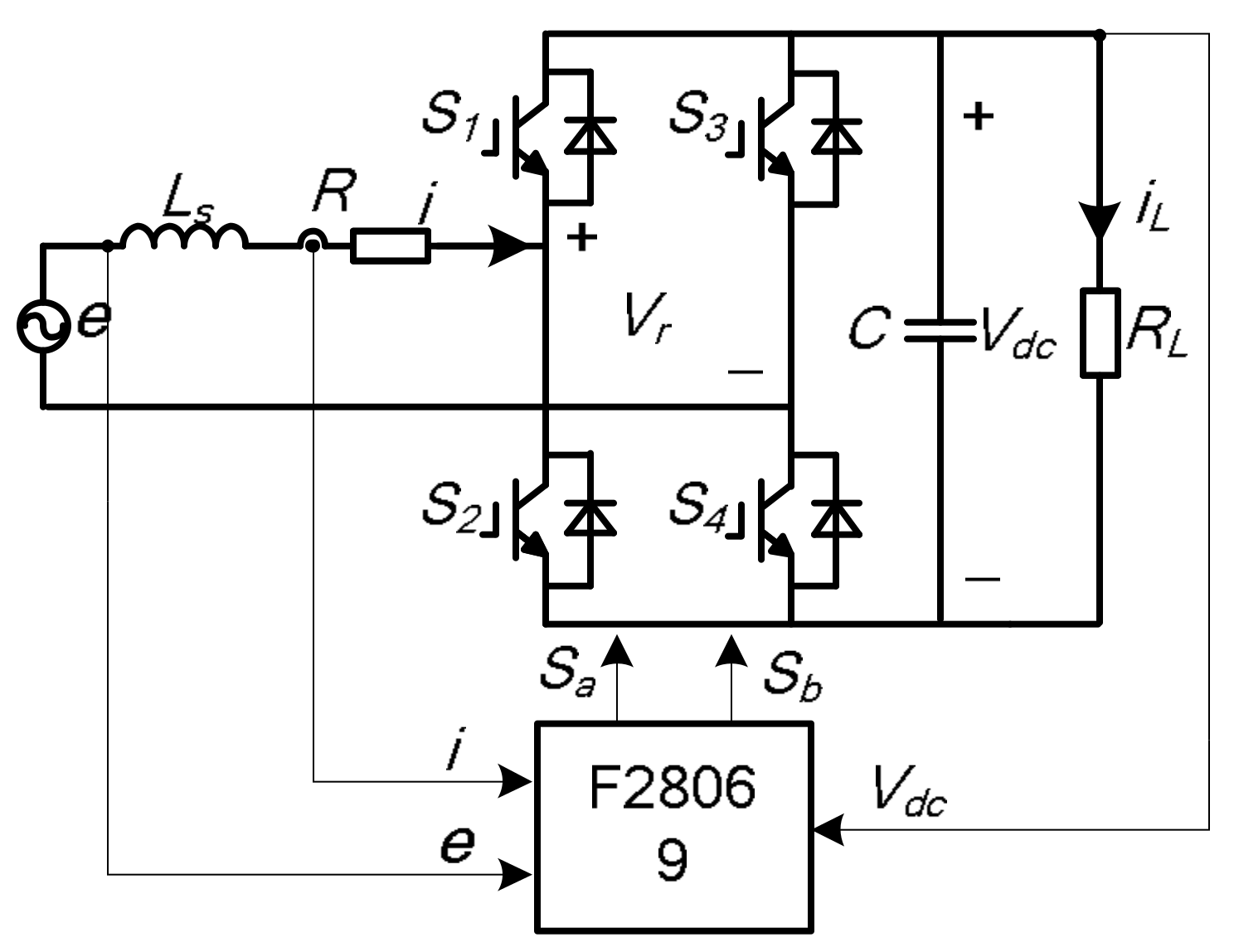
2. Modeling of the Converter

Figure 1 shows the single-phase voltage source rectifier. The equation for the converter can be described as:

$$L_s\frac{di}{dt}=e-Ri-V_r$$

(1)

where e, V_r and i are the grid voltage, converter voltage, and grid current, respectively, and R and L_s are the equivalent series resistance and filter inductance, respectively.

According to the Forward Euler method, di/dt can be approximated as:

$$\frac{di}{dt}=\frac{i(k+1)-i(k)}{T}$$

(2)

where T is the sampling period.

By substituting (2) into (1) [7], the discrete-time model of the S-VSR can be obtained as:

$$i(k+1)=(1-\frac{RT}{L_s})i(k)+\frac{T}{L_s}[e(k)-V_r(k)]$$

(3)

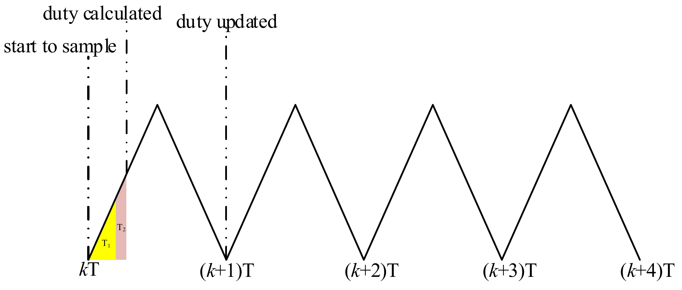
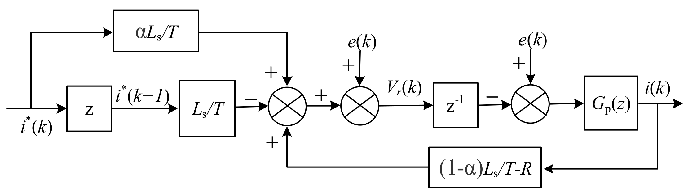
3. The Principle of the Proposed Method

Stability is essential for control systems and it is also very important that measured current, i(k), tracks the reference value, i*(k), precisely. Namely, current tracking error, Δi(k), converges to zero. The Lyapunov theorem is powerful in ensuring the stability of all control systems.

Tracking error, Δi(k), is defined as:

$$\Delta i(k)=i(k)-i^{*}(k)$$

(4)

As [23] depicts, the discrete Lyapunov function, L(x(k)), should satisfy the following properties to ensure the stability of the control system:

(1)

L(0) = 0;

(2)

L(x(k)) > 0 for all x(k) ≠ 0;

(3)

L(x(k)) → ∞ as ‖x(k)‖ → ∞;

(4)

ΔL(x(k)) < 0 for all x(k) ≠ 0.

Thus, the discrete Lyapunov function, L(Δi(k)), can be defined as:

$$L(\Delta i(k))=\frac{1}{2}\Delta i^2(k)$$

(5)

From (4) and (5), ΔL(Δi(k)) can be expressed as:

$$\begin{array}{ll}\Delta L(\Delta i(k))& =L(\Delta i(k+1))-L(\Delta i(k))\\ & =\frac{1}{2}{\left[i(k+1)-i^{*}(k+1)\right]}^2-\frac{1}{2}{\left[i(k)-i^{*}(k)\right]}^2\end{array}$$

(6)

To satisfy the Lyapunov stability theorem and ensure that current tracking error converges to zero, we defined the following relationship:

$$i(k+1)-i^{*}(k+1)=\alpha \left[i(k)-i^{*}(k)\right]$$

(7)

Substituting (7) into (6), the following expression for ΔL(Δi(k)) can be obtained:

$$\begin{array}{ll}\Delta L(\Delta i(k))& =L(\Delta i(k+1))-L(\Delta i(k))\\ & =\frac{1}{2}({\alpha }^2-1){\left[i(k)-i^{*}(k)\right]}^2\end{array}$$

(8)

It is apparent that the system is stable if α is chosen as:

$$-1<\alpha <1$$

(9)

The control law of the presented method can be written with (3) and (7) as:

$$\begin{array}{ll}{V}_r(k)& =e(k)+(\frac{L_s}{T}-R)i(k)\\ & -\frac{L_s}{T}{i}^{*}(k+1)-\alpha \frac{L_s}{T}\left[i(k)-i^{*}(k)\right]\end{array}$$

(10)

It is clearly depicted that when α = 0, (10) is the prediction model of the conventional deadbeat control method.

One of the key issues related to the method presented is how to decide the best control coefficient, α, to use in the prediction model. Selection and analysis of the control coefficient is described in the following section.

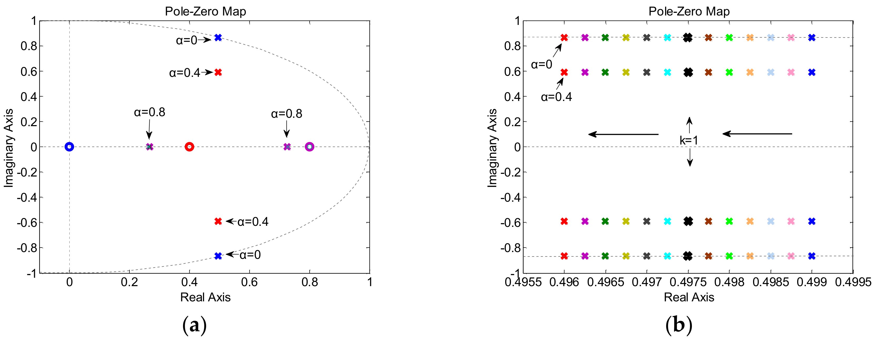
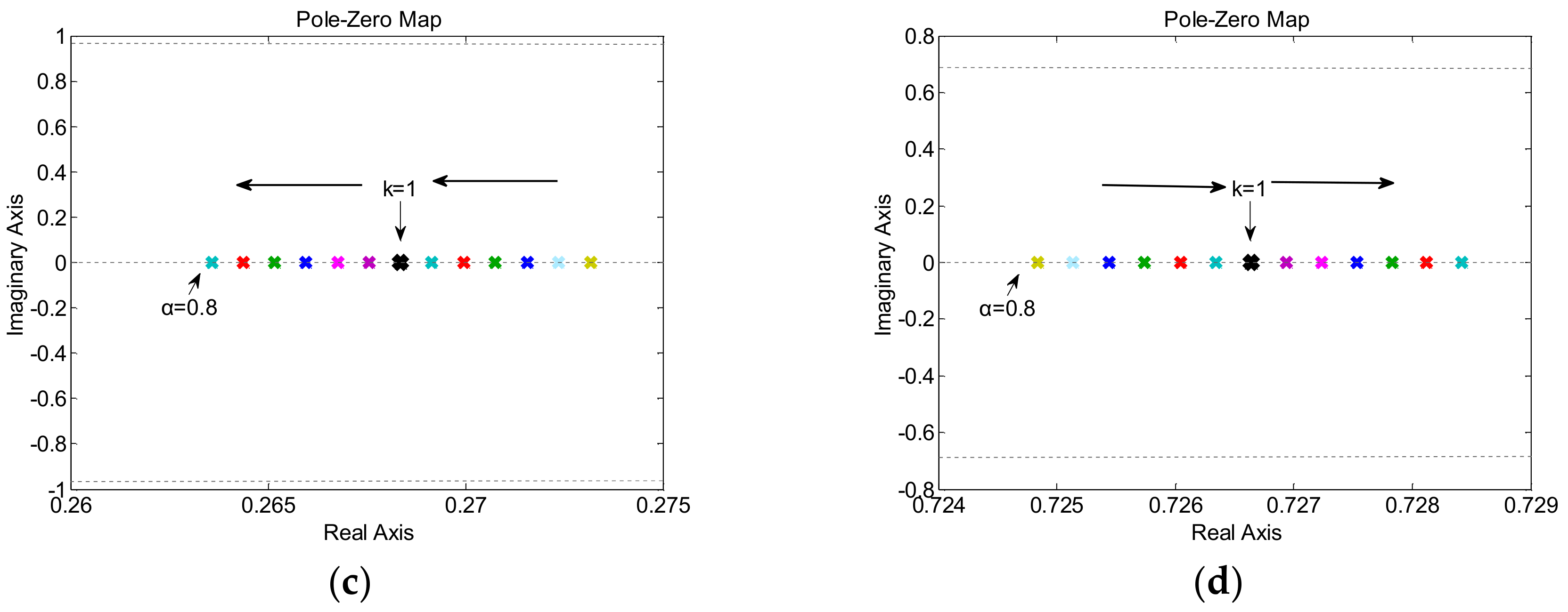
4. Selection and Analysis of Control Coefficient

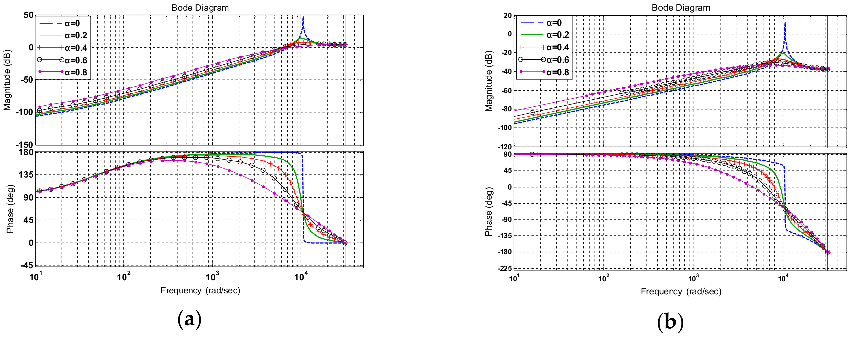
4.1. Influence of Stability

When a digital control strategy is applied, a delay always exists in the control system, including the sampling time. The calculation time of the control strategy and, more importantly, duty is always updated in each subsequent sampling period. Figure 2 shows what happens when a delay exists in a control system. According to the datasheet of TI and the experimental results, the total sampling and convention time was T₁ = 8.6 μs, and the calculation time of the control strategy was T₂ = 3.1 μs. As the switching period was 100 μs, it was enough for all of the sampling and calculations in the switching period. Because the duty calculated in the kth switching period was updated at the beginning of the (k + 1)th switching period, a one sampling period delay was assumed to analyze the problem.

A discrete control block diagram of the proposed control strategy under a S-VSR is shown in Figure 3.

In the S Domain, the transfer function of the controlled object in the current loop can be expressed as:

$$G_p(s)=\frac{1}{s{L}_s+R}$$

(11)

The delay of one sampling period is modeled by the z⁻¹ block. The zero-order hold (ZOH) equivalence transfer function of G_p(s) is shown as (11) [9].

$$\begin{array}{ll}{G}_p(z)& =(1-z^{-1})Z\left[\frac{G_p(s)}{s}\right]\\ & =\frac{T}{L_s}\frac{1}{z-(1-RT/L_s)}\end{array}$$

(12)

The closed-loop transfer function of the current loop, with regard to e(k), which functioned as a disturbance, can be described as:

$$\begin{array}{ll}G(z)& =\frac{i(k)}{i^{*}(k)}=\frac{(k_{3}z-k_1)z^{-1}{G}_p(z)}{1+k_2{z}^{-1}{G}_p(z)}\\ & =\frac{z-\alpha }{z^2-(1-R\frac{T}{L_s})z+(1-\alpha -R\frac{T}{L_s})}\end{array}$$

(13)

where k₁ = αL_s/T, k₂ = (1 − α)L_s/T − R, and k₃ = L_s/T.

In order to ensure the stability of the system, the following should be satisfied:

$$0<1-\alpha -RT/L_s<1$$

(14)

In this paper, the system parameters were selected as L_s = 3.2 mH, R = 0.3 Ω, and T = 0.0001 s. Based on (9) and (14), the control coefficient, α, could be limited as:

$$-0.005<\alpha <0.995$$

(15)

4.2. Influence of Steady-State Error

Based on the closed-loop transfer function of the current loop shown in Figure 3, with e(k) representing a disturbance, we can derive the error transfer function for i*(k) as follows:

$$E_{nn}(z)=\frac{i^{*}(k)-i(k)}{i^{*}(k)}=\frac{z^2-(2-R\frac{T}{L_s})z+(1-R\frac{T}{L_s})}{z^2-(1-R\frac{T}{L_s})z+(1-\alpha -R\frac{T}{L_s})}$$

(16)

When i*(k) = 0, we derive the disturbance error transfer function for e(k).

$$D_{ss}(z)=\frac{i^{*}(k)-i(k)}{e(k)}=\frac{\frac{T}{L_s}(z-1)}{z^2-(1-R\frac{T}{L_s})z+(1-\alpha -R\frac{T}{L_s})}$$

(17)

Thus, the steady state error E(z) can be described as:

$$E(z)=E_{nn}(z)i^{*}(k)-D_{ss}(z)e(k)$$

(18)

It is supposed that i*(k) and e(k) are all sinusoidal, and E(z) can be written as:

$$\begin{array}{ll}E(z)=& I\frac{z^2-(2-R\frac{T}{L_s})z+(1-R\frac{T}{L_s})}{z^2-(1-R\frac{T}{L_s})z+(1-\alpha -R\frac{T}{L_s})}\frac{z\sin ({\omega }_{i}T)}{z^2-2z\cos ({\omega }_{i}T)+1}-\\ & E\frac{\frac{T}{L_s}(z-1)}{z^2-(1-R\frac{T}{L_s})z+(1-\alpha -R\frac{T}{L_s})}\frac{z\sin ({\omega }_{e}T)}{z^2-2z\cos ({\omega }_{e}T)+1}\end{array}$$

(19)

A bode diagram of E_nn(z) and D_ss(z) is given in Figure 4.

As shown in Figure 4a, the gain in E_nn(z) was among 10⁻⁵~10⁻³ when the working frequency was 50 Hz, which can be regarded as tracking without steady state error. From Figure 4b, we can see that the gain in D_ss(z) was among 10⁻⁵~10⁻³ when the working frequency was 50 Hz. As α became larger, the gain in E_nn(z) and D_ss(z) was nearly the same for all working frequencies, which implies that the value of α did not influence the steady-state performance of the control system.

Based on the final value theorem of discrete control systems, we can derive steady state error e(∞) as:

$$e(\infty )=\underset{z\to 1}{\lim }(z-1)E(z)=0$$

(20)

4.3. Influence of Robustness

To investigate the influence of the inductance parameter mismatch on robustness, the pole locus was analyzed, with variations in the nominal value, L_s, based on the typical value of α.

By replacing L_s with the actual value of the inductance, L_a, the closed-loop transfer function, G(z)_a, of the current loop can be expressed as:

$$\begin{array}{ll}G{(z)}_a& =\frac{i(k)}{i^{*}(k)}=\frac{(k_{3a}z-k_{1a})z^{-1}{G}_p{(z)}_a}{1+k_{2a}{z}^{-1}{G}_p{(z)}_a}\\ & =\frac{z-\alpha }{z^2-(1-R\frac{kT}{L_s})z+(1-\alpha -R\frac{kT}{L_s})}\end{array}$$

(21)

where k_1a = αL_a/T, k_2a = (1 − α)L_a/T − R, k_3a = L_a/T, and k = L_s/L_a, denoting the difference between the inductance value used in the controller and the actual value. Figure 5 depicts the zero-pole graph of the variation in k with different values of α. p1,p2,p3 and p4 were all poles of G(z)_a.

It can be observed from Figure 5 that when α = 0, the poles were much closer to the unit circle, regardless of whether L_a was smaller or larger than L_s, and the system had weaker robustness. When α was selected within the range calculated in (15), the poles were always in the unit cycle, regardless of the size of L_a. The influence of the equivalent series resistance R parameter mismatch on robustness could be analyzed in the same way, with k defined as k = R_a/R_s, where R_a and R_s were the actual value and the ideal value, respectively. Therefore, from Figure 5, we can see that the proposed control had better robustness than the conventional deadbeat control.

4.4. Selection of α

According to (13), we can obtain the damping ratio as follows:

$$\xi =\frac{1-R\frac{T}{L_S}}{2\sqrt{1-\alpha -R\frac{T}{L_s}}}$$

(22)

The better damping ratio in the industrial application was 0.707, thus α was chosen as 0.52 by solving (23):

$$\xi =\frac{1-R\frac{T}{L_S}}{2\sqrt{1-\alpha -R\frac{T}{L_s}}}=0.707$$

(23)

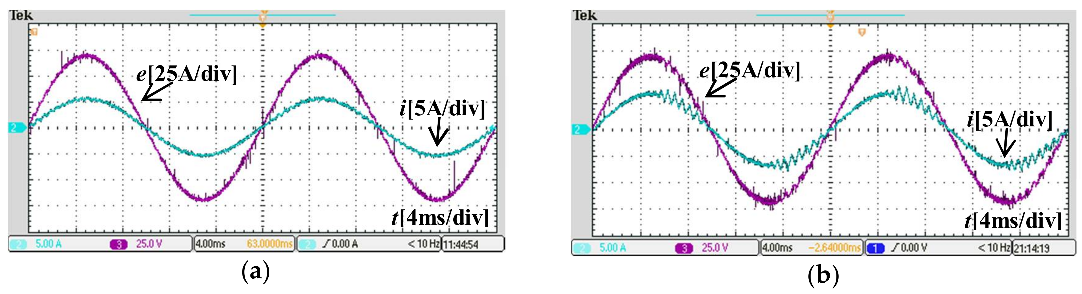
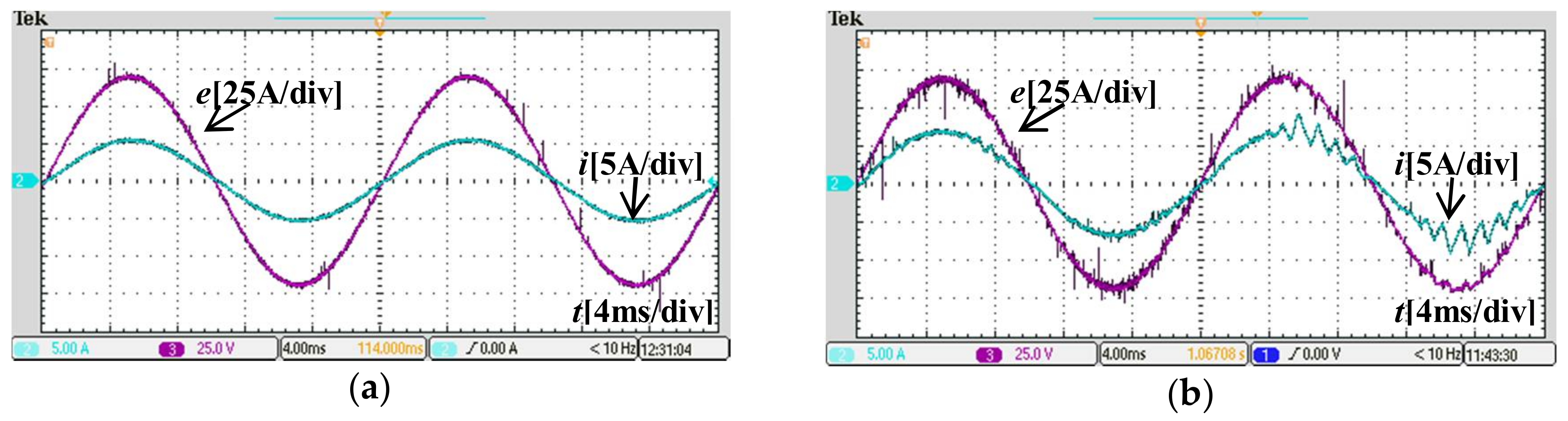
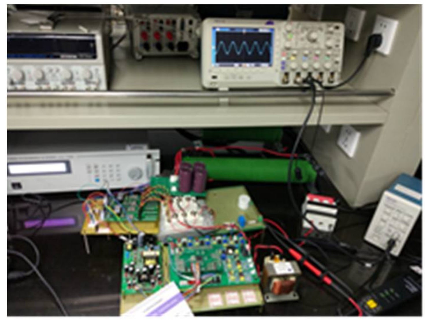
5. Experimental Results

The experimental test was performed under the S-VSR prototype described in Figure 6. The control strategy was achieved in a DSP system with TMS320F28069 (Texas Instruments, Dallas, TX, USA). The waveforms of the measured current and its analysis were obtained using a Tektronix oscilloscope and power analyzer. The system parameters are given in

Table 1. Experimental results.

Varible	Symbol	Value
The grid voltage (RMS)	e	50 V/50 Hz
Filter inductance	Ls	3.1 mH
Equivalent series resistance	R	0.3 Ω
DC side capacitor	C	1000 μF
Sampling period	T	1 × e−4 s
Switching frequency	f	10 kHz

. In order to test availability, we gave the reference value of the filter inductance directly.

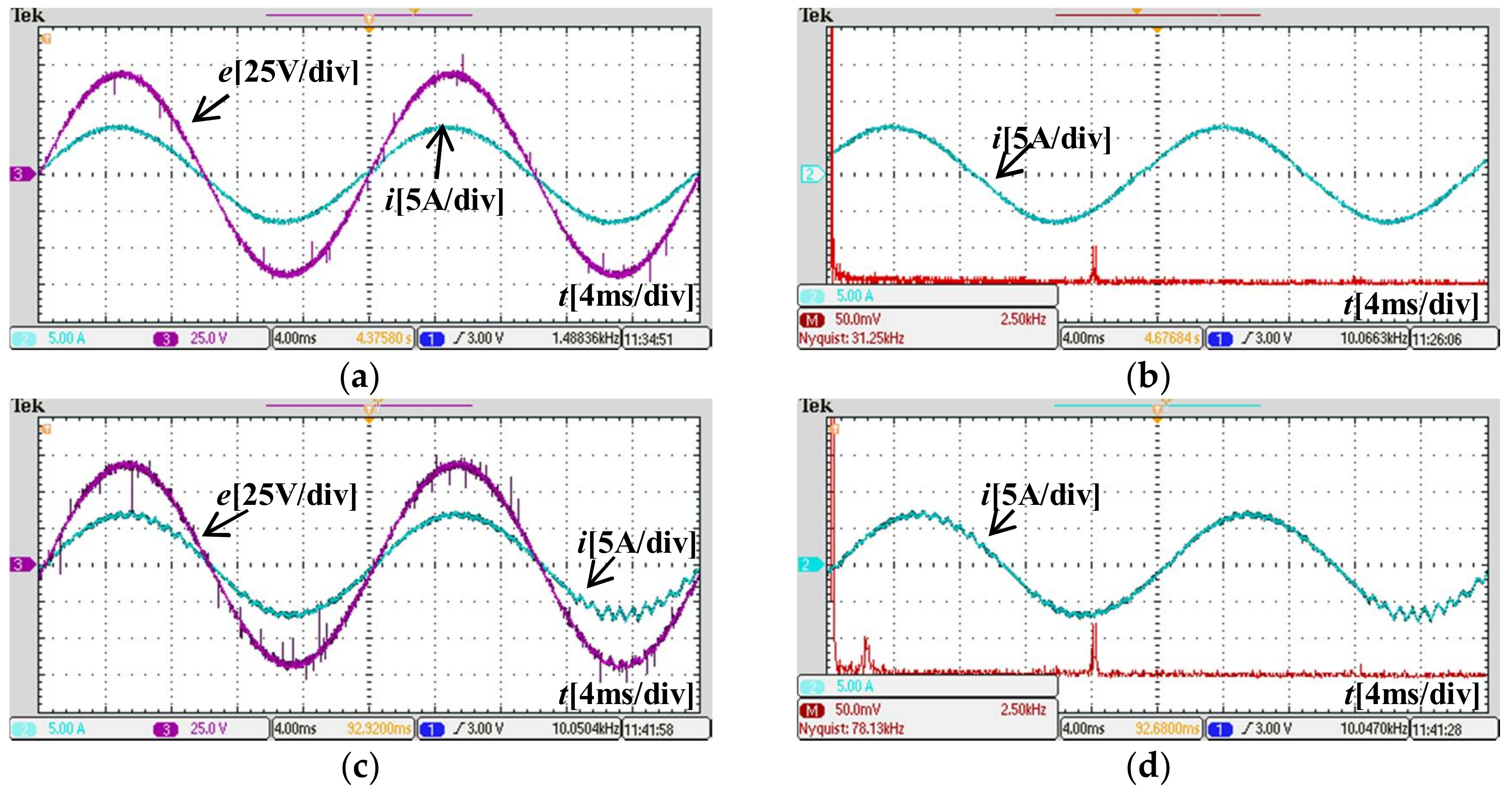
5.1. Steady-State Performance Tests

Figure 7a,b shows the grid current behavior of the presented method when the reference value was 6.8 A, with unity power factor. The experimental results showed better steady-state behavior for the proposed method. The grid current was highly sinusoidal, with total harmonic distortion (THD) of 1.86%. Figure 7c,d describes the tested results of the traditional deadbeat control. As observed in the experimental results, there was oscillation in the system, with a noisy current and a THD of 4.1%, which may have been caused by a delay. From Figure 7, we can see that the error correction improved steady-state performance.

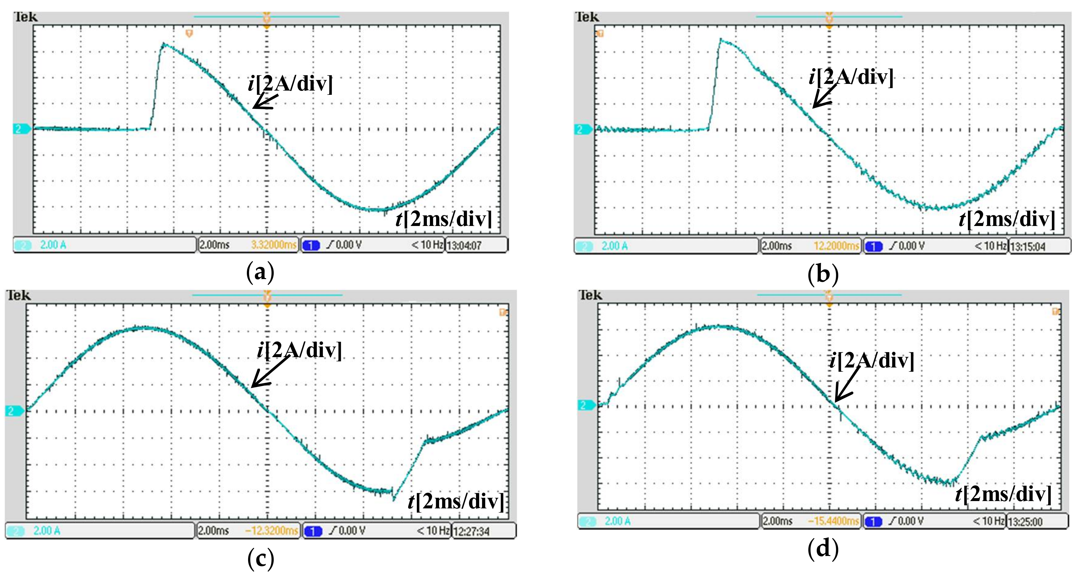
5.2. Dynamic Response Tests

An important aspect to any control system is the dynamic response to changes in the reference value [23]. Figure 8 shows the system behavior for a current with a reference step from a 0 A to a 6 A peak and from a 6 A to a 3 A peak, for the proposed control method and the conventional deadbeat control method. Figure 8a shows that the current reached a steady state within 460 μs, compared to 395 μs in Figure 8b. The transient time in Figure 8c was 664 μs and in Figure 8d was 564 μs. Compared to the traditional deadbeat control method, the dynamic response of the proposed control strategy was slightly slower with smaller amounts.

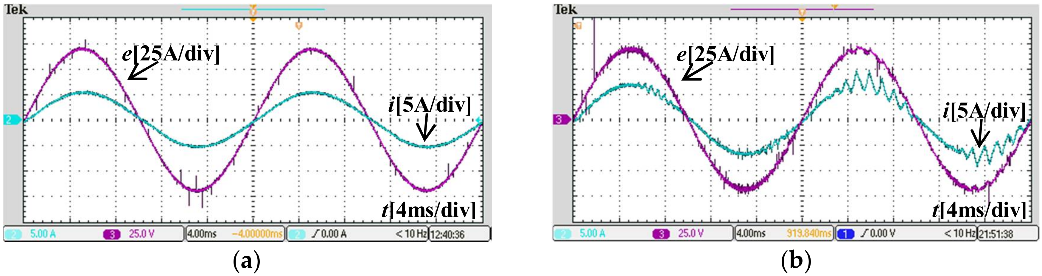
5.3. Investigation of Robustness

The system parameters, especially filter inductance, varied with temperature and other environmental factors. The performance of the proposed method and deadbeat control method, with differing levels of error between the modeled and the real inductance, in the range of −30% to 30%, is given in Figure 9, Figure 10, Figure 11 and Figure 12, respectively. It was found that the variation in inductance led to increased current THD, but at lower levels using the proposed control method. However, there were large current oscillations with higher levels of THD using the conventional deadbeat control method when inductance varied. These experimental results show stronger robustness using the proposed control method.

6. Conclusions

To overcome the weak robustness of conventional deadbeat control methods, this paper proposed a robust digital control strategy using error correction based on the discrete Lyapunov theorem. The proposed method introduced error correction into the prediction model to increase robustness. More importantly, the discrete Lyapunov theorem was added to the model to improve global stability. Theoretical analyses using transfer functions and zero-pole graphs, and experimental results under a single-phase voltage source rectifier system, demonstrated that the proposed method not only behaved with stronger robustness, but also led to a high sinusoidal current with lower THD, while still retaining a fast, dynamic response and minimal level of tracking error. The proposed method shows encouraging prospective applications to numerous model-based control strategies.

References

1. Shahid, A. An overview of control architecture for next generation smart grids. In Proceedings of the 2017 19th International Conference on Intelligent System Application to Power Systems (ISAP), San Antonio, TX, USA, 17–20 September 2017; pp. 1–5. [Google Scholar]
2. Gai, W.; Chen, D.; Yin, J.; Chen, L. High-speed maglev parallel control and management system-overview and framework. In Proceedings of the 2014 International Conference on Informative and Cybernetics for Computational Social Systems (ICCSS), Qingdao, China, 9–10 October 2014; pp. 24–28. [Google Scholar]
3. Li, P.; Song, Y.D.; Li, D.Y.; Cai, W.C.; Zhang, K. Control and Monitoring for Grid-Friendly Wind Turbines: Research Overview and Suggested Approach. IEEE Trans. Power Electron. 2015, 30, 1979–1986. [Google Scholar] [CrossRef]
4. Calderon-Lopez, G.; Villarruel-Parra, A.; Kakosimos, P.; Ki, S.K.; Todd, R.; Forsyth, A.J. Comparison of digital PWM control strategies for high-power interleaved DC–DC converters. IET Power Electron. 2018, 11, 391–398. [Google Scholar] [CrossRef]
5. Chattopadhyay, S.; Das, S. A Digital Current-Mode Control Technique for DC–DC Converters. IEEE Trans. Power Electron. 2006, 21, 1718–1726. [Google Scholar] [CrossRef]
6. Pan, S.Z.; Jain, P.K. A Low-Complexity Dual-Voltage-Loop Digital Control Architecture with Dynamically Varying Voltage and Current References. IEEE Trans. Power Electron. 2014, 29, 2049–2060. [Google Scholar] [CrossRef]
7. Qi, C.; Chen, X.; Tu, P.; Wang, P. Deadbeat control for a single-phase cascaded H-bridge rectifier with voltage balancing modulation. IET Power Electron. 2018, 11, 610–617. [Google Scholar] [CrossRef]
8. Xueguang, Z.; Wenjie, Z.; Jiaming, C.; Dianguo, X. Deadbeat Control Strategy of Circulating Currents in Parallel Connection System of Three-Phase PWM Converter. IEEE Trans. Energy Convers. 2014, 29, 406–417. [Google Scholar]
9. Hung, G.K.; Chang, C.-C.; Chen, C.-L. Analysis and implementation of a delay compensated deadbeat current controller for solar inverters. IEE Proc. Circuits Devices Syst. 2001, 148, 279–286. [Google Scholar] [CrossRef]
10. Stumper, J.F.; Hagenmeyer, V.; Kuehl, S.; Kennel, R. Deadbeat Control for Electrical Drives: A Robust and Performant Design Based on Differential Flatness. IEEE Trans. Power Electron. 2015, 30, 4585–4596. [Google Scholar] [CrossRef]
11. SLarrinaga, A.; Vidal, M.A.R.; Oyarbide, E.; Apraiz, J.R.T. Predictive control strategy for dc/ac converters based on direct power control. IEEE Trans. Ind. Electron. 2007, 54, 1261–1271. [Google Scholar] [CrossRef]
12. Rodriguez, J.; Kazmierkowski, M.P.; Espinoza, J.R.; Zanchetta, P.; Abu-Rub, H.; Young, H.A.; Rojas, C.A. State of the art of finite control set model predictive control in power electronics. IEEE Trans. Ind. Inform. 2013, 9, 1003–1016. [Google Scholar] [CrossRef]
13. Bibian, S.; Jin, H. High Performance Predictive Dead-Beat Digital Controller for DC Power Supplies. IEEE Trans. Power Electron. 2002, 17, 420–427. [Google Scholar] [CrossRef]
14. Bode, G.H.; Loh, P.C.; Newman, M.J.; Holmes, D.G. An improved robust predictive current regulation algorithm. IEEE Trans. Ind. Appl. 2005, 41, 1720–1733. [Google Scholar] [CrossRef]
15. Siami, M.; Abbaszadeh, A.; Khaburi, D.A.; Rodriguez, J. Robustness improvement of predictive current control using prediction error correction for permanent magnet synchronous machines. IEEE Trans. Ind. Electron. 2016, 63, 3458–3466. [Google Scholar] [CrossRef]
16. Di Cairano, S.; Heemels, W.P.M.H.; Lazar, M.; Bemporad, A. Stabilizing Dynamic Controllers for Hybrid Systems: A Hybrid Control Lyapunov Function Approach. IEEE Trans. Autom. Control 2014, 59, 2629–2643. [Google Scholar] [CrossRef]
17. Wang, J.W.; Wu, H.N.; Li, H.X. Fuzzy Control Design for Nonlinear ODE-Hyperbolic PDE-Cascaded Systems: A Fuzzy and Entropy-Like Lyapunov Function Approach. IEEE Trans. Fuzzy Syst. 2014, 22, 1313–1324. [Google Scholar] [CrossRef]
18. Furqon, R.; Chen, Y.J.; Tanaka, M.; Tanaka, K.; Wang, H.O. An SOS-Based Control Lyapunov Function Design for Polynomial Fuzzy Control of Nonlinear Systems. IEEE Trans. Fuzzy Syst. 2017, 25, 775–787. [Google Scholar] [CrossRef]
19. Sefa, I.; Ozdemir, S.; Komurcugil, H.; Altin, N. Comparative study on Lyapunov-function-based control schemes for single-phase grid-connected voltage-source inverter with LCL filter. IET Renew. Power Gener. 2017, 11, 1473–1482. [Google Scholar] [CrossRef]
20. Kwak, S.; Yoo, S.J.; Park, J. Finite control set predictive control based on Lyapunov function for three-phase voltage source inverters. IET Power Electron. 2014, 7, 2726–2732. [Google Scholar] [CrossRef]
21. Parvez, M.; Mekhilef, S.; Tan, N.M.L.; Akagi, H. A robust modified model predictive control (MMPC) based on Lyapunov function for three-phase active-front-end (AFE) rectifier. In Proceedings of the 2016 IEEE Applied Power Electronics Conference and Exposition (APEC), Long Beach, CA, USA, 18–24 March 2016; pp. 1163–1168. [Google Scholar]
22. Akter, M.P.; Mekhilef, S.; Tan, N.M.L.; Akagi, H. Modified model predictive control of a bidirectional AC-DC converter based on Lyapunov function for energy storage systems. IEEE Trans. Ind. Electron. 2016, 63, 704–715. [Google Scholar] [CrossRef]
23. Du, G.; Liu, Z.; Du, F.; Li, J. Performance Improvement of Model Predictive Control Using Control Error Compensation for Power Electronic Converters Based on the Lyapunov Function. J. Power Electron. 2017, 17, 983–990. [Google Scholar]
Figure 1. Single-phase voltage source rectifier.
Energies 11 00848 g001
Figure 2. Description of delay exists in the control system.
Energies 11 00848 g002
Figure 3. Inner current loop control block diagram.
Energies 11 00848 g003
Figure 4. Bode diagram of steady-state error: (a) Enn(z); (b) Dss(z).
Energies 11 00848 g004
Figure 5. Pole locus diagram of G(z)a with variations in k (from 0.4 to 1.6, in increments of 0.1). (a) The whole sight of pole locus; (b) The pole (p1 and p2) locus based on α = 0 and α = 0.4; (c) The pole (p3) locus based on α = 0.8; (d) The pole (p4) locus based on α = 0.8.
Energies 11 00848 g005aEnergies 11 00848 g005b
Figure 6. The experimental prototype.
Energies 11 00848 g006
Figure 7. Steady-state test results using the proposed method (α = 0.52) and the conventional deadbeat control method. (a) The voltage and current waveforms (α = 0.52); (b) The harmonic spectrum of the current (α = 0.52); (c) The voltage and current waveforms of the conventional deadbeat control; (d) The harmonic spectrum of the current of the conventional deadbeat control.
Energies 11 00848 g007
Figure 8. Current behavior during the reference step change from a 0 to 6 A peak and from a 6 A to 3 A peak. (a) 0 A to 6 A peak with the proposed control method (α = 0.52); (b) 0 A to 6 A peak with the conventional deadbeat control method; (c) 6 A to 3 A peak with the proposed control method (α = 0.52); (d) 6 A to 3 A peak with the conventional deadbeat control method.
Energies 11 00848 g008
Figure 9. Current behavior when the inductance had a mismatch of −30%. (a) Under the proposed control method (α = 0.52); (b) Under the conventional deadbeat control method.
Energies 11 00848 g009
Figure 10. Current behavior when the inductance had a mismatch with −15%. (a) Under the proposed control method (α = 0.52); (b) Under the conventional deadbeat control method.
Energies 11 00848 g010
Figure 11. Current behavior when the inductance had a mismatch with +15%. (a) Under the proposed control method (α = 0.52); (b) Under the conventional deadbeat control method.
Energies 11 00848 g011
Figure 12. Current behavior when the inductance had a mismatch with +30%. (a) Under the proposed control method (α = 0.52); (b) Under the conventional deadbeat control method.
Energies 11 00848 g012