Lambda-Based Data Processing Architecture for Two-Level Load Forecasting in Residential Buildings

Abstract

Building energy management systems (BEMS) have been intensively used to manage the electricity consumption of residential buildings more efficiently. However, the dynamic behavior of the occupants introduces uncertainty problems that affect the performance of the BEMS. To address this uncertainty problem, the BEMS may implement load forecasting as one of the BEMS modules. Load forecasting utilizes historical load data to compute model predictions for a specific time in the future. Recently, smart meters have been introduced to collect electricity consumption data. Smart meters not only capture aggregation data, but also individual data that is more frequently close to real-time. The processing of both smart meter data types for load forecasting can enhance the performance of the BEMS when confronted with uncertainty problems. The collection of smart meter data can be processed using a batch approach for short-term load forecasting, while the real-time smart meter data can be processed for very short-term load forecasting, which adjusts the short-term load forecasting to adapt to the dynamic behavior of the occupants. This approach requires different data processing techniques for aggregation and individual of smart meter data. In this paper, we propose Lambda-based data processing architecture to process the different types of smart meter data and implement the two-level load forecasting approach, which combines short-term and very short-term load forecasting techniques on top of our proposed data processing architecture. The proposed approach is expected to enhance the BEMS to address the uncertainty problem in order to process data in less time. Our experiment showed that the proposed approaches improved the accuracy by 7% compared to a typical BEMS with only one load forecasting technique, and had the lowest computation time when processing the smart meter data.

1. Introduction

Buildings have been identified as entities that consume a significant portion of electricity [1,2,3]. The residential building, as one building type, consumed 38% of total U.S. electricity in 2014 [4], which makes it a significant prominent electricity consumer in the building sector. A significant portion of the energy consumption in residential buildings is used for the services that maintain the occupants’ comfort, such as heat, ventilation, and air conditioning (HVAC) and lighting systems [5,6]. The high electricity consumption of residential buildings will be a burden for electricity generation and will lead to severe impacts on the global environment. Current electricity generation, which consists of oil-fuel-based electricity, and the rise of renewable energy sources with unstable electricity provision has become a limitation to providing the electricity demands of residential buildings. This situation increases the need to manage the electricity consumption of residential buildings more efficiently. Building energy management systems (BEMS) are one solution used by residential building operators to efficiently balance the electricity demand and electricity supply of buildings and to minimize the electricity cost, while maintaining the occupant’s comfort [5,7]. Recent research has been conducted to study the implementation of BEMSs in residential buildings [8,9,10,11,12,13]. However, due to the dynamic nature of occupants’ behavior, the electricity consumption may be different over time [14,15,16]. This dynamic behavior introduces an uncertainty problem that may reduce the performance of the BEMS.

One solution to address this uncertainty problem for BEMSs is the introduction of a forecasting module. A forecasting module enables the BEMS to predict the electricity demand of the building for a specific time ahead [17]. The forecasting module implements a load forecasting technique based on several data—e.g., historical load data, weather forecasts, the calendar and the behavior of the occupants—to develop a prediction model for the electricity demand. These data can be collected by an internal system (e.g., meters and sensors deployed inside the residential building) and an external system (e.g., weather forecasts from weather stations) and are provided to the BEMS with different time windows. With the forecasting module, the BEMS may predict the electricity demand in advance and determine the best dispatch strategy for electricity supply to meet the predicted electricity demand at a given time.

Recently, the use of conventional meters to record electricity consumption has been replaced by smart meter technology [18,19]. The conventional meter records the electricity consumption in the form of aggregation data (e.g., one-day aggregation data). This aggregation data may capture a less dynamic aspect of the occupants’ behavior. Smart meters offer the capability of not only capturing aggregation data, but also of capturing more granular information on electricity consumption within short time windows (e.g., 15 min, 30 min, 1 h, one day or near real-time) and can reach the individual level of the customers. 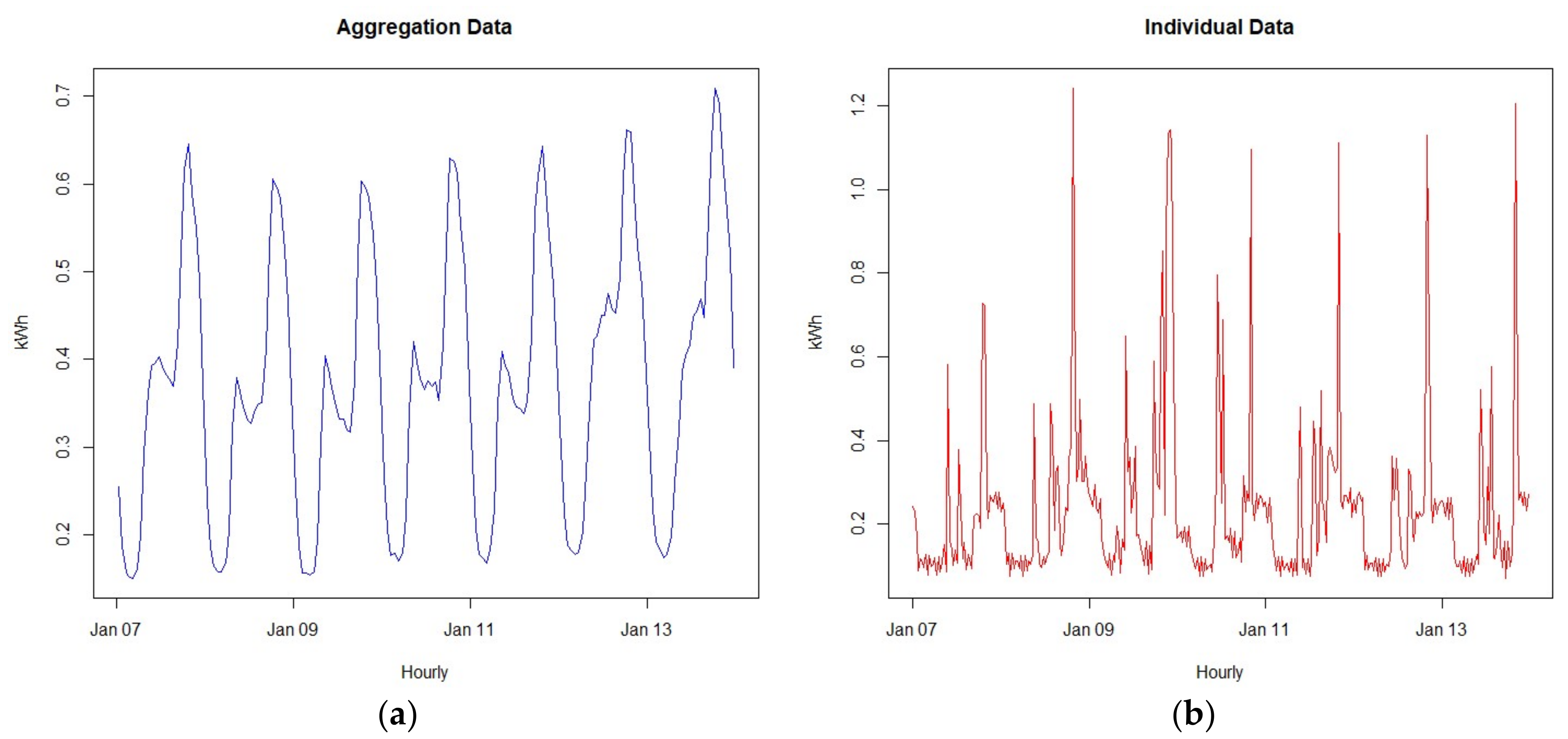The authors in [20] showed two forms of smart meter data, namely aggregation data and individual data. Figure 1 illustrates the visualization of aggregation data in the left graph and individual data in the right graph. From Figure 1, we can see that the individual data shows an irregular pattern which represents the dynamic behavior of the occupants. Data analysis techniques have been developed to utilize the aggregation and individual data separately [21]. However, incorporating the aggregation and individual data into one analysis process for a load forecasting technique may enhance the performance of the BEMS when addressing the uncertainty problem.

Various researches have been conducted to study the usage of the aggregation data and the individual data of the smart meter for load forecasting techniques in BEMS. In [3], the authors considered the randomness behavior of the occupants, which may affect the accuracy of load forecasting. They develop a technique to extract features from the aggregation data and use them for long-term load forecasting. However, they did not consider the randomness behavior of the occupants that happens in a shorter period (e.g., one hour). In [10], the authors studied the impact of real-time smart meter data on the accuracy of the load forecasting technique. Their results show that the one-hour period of smart meter data is a more effective model for load forecasting. However, the number of smart meter data and the velocity of the data may impact the timely processing of the data. The increasing number of smart meter data and the narrow time constraint of the data velocity may increase the processing time for this data.

An advanced approach is proposed by the authors in [22], enabling long-term model prediction to be adjusted by real-time data in every time unit, that is, the dynamic behavior of the occupants changes the system status. The proposed approach introduces a strategy that includes prediction, long-term scheduling and a real-time controller (RTC). The prediction utilizes historical load data incorporated with the external factors of the building—such as pricing schema, weather, etc.—and develops a long-term model load forecast. The long-term scheduling utilizes long-term model prediction to compute control parameters for the building components for N hours ahead. The RTC is used to adapt the dynamic changes of electricity usage in real-time and adjust the long-term forecasting model for (N-1) hours. The proposed approach introduces the concept of two-level load forecasting, which benefits the model prediction controller (MPC) technique. The MPC technique is widely deployed by the BEMS to control the electricity consumption of the HVAC and lighting system of the residential building [23,24]. The two-level load forecasting enables the MPC to optimize the electricity consumption of the HVAC and lighting system in the dynamically changing environment. With this strategy, they claim success in reducing the total cost of building energy by about 15%. However, their approach consumes high computing power since the RTC has to re-compute the long-term forecasting model following the real-time data for each time unit.

In this paper, we propose a data processing architecture to reduce the processing time of the load forecasting computation. Since there are smart meter data that are computed once for short-term load forecasting and real-time smart meter data which is computed more frequently for very short-term load forecasting, we adopted Lambda architecture and introduced a two-level load forecasting technique that utilizes our proposed data processing architecture. Our proposed data processing architecture separates the process layer of the smart meter data based on the time processing requirement. Our contributions in this paper are as follows: (1) We introduce two-level load forecasting to enable the system to adapt to the dynamic behavior of the occupants; (2) We propose a Lambda-like architecture to process the smart meter data following the different time processing requirements; (3) We evaluate our system using a real dataset by comparing the cost reduction and time processing to show the advantages of our proposed architecture.

The rest of the paper is ordered as follows. In Section 2, we discuss the BEMS control approaches and the framework considered in this paper. In Section 3, we discuss the two-level load forecasting technique and the proposed Lambda-like data processing architecture. In Section 4, we discuss the evaluation of our proposed data processing architecture. In Section 5, we review the previous work related to our work, and we conclude our paper in Section 6.

2. Preliminaries

2.1. Overview of the BEMS

To design the data processing architecture, we considered the control approaches that may apply to the BEMS. The BEMS is used by a building operator that manages a group of residential buildings. The group of residential buildings is equipped with central electricity production that contains renewable energy sources (RESs) and energy storage systems (ESSs) and has a connection to the grid. Each building has controllable loads that are managed by the BEMS to support the occupants’ comfort.

2.1.1. BEMS Control Approaches

Based on the microgrid control classification, there are three control approaches for energy management systems, namely the centralized, decentralized and distributed approach [25].

● Centralized BEMS

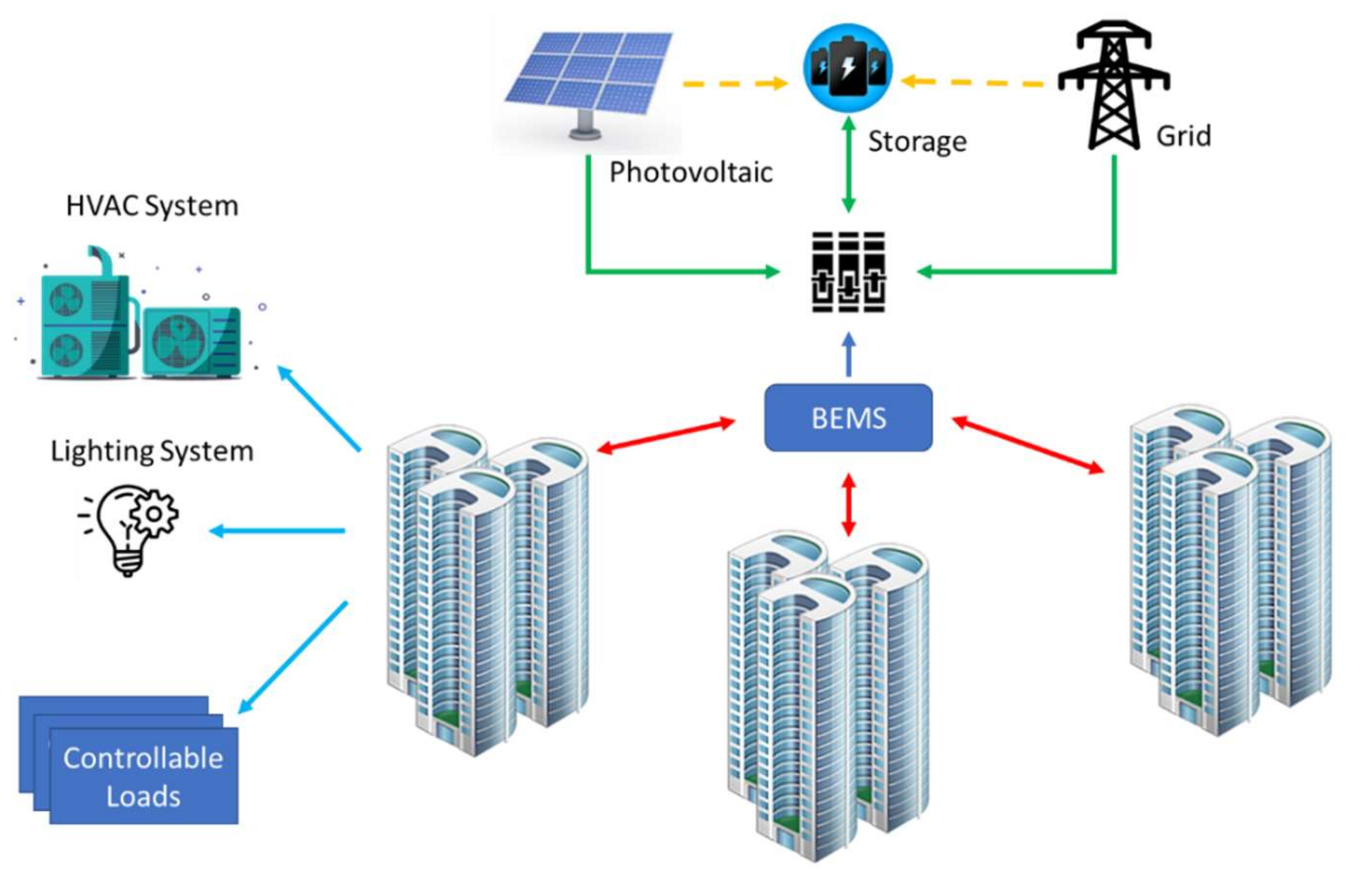
In residential buildings, centralized BEMS has a special location designed by the building operator to control and manage the global controllable loads and generation devices of the buildings. Under this approach, the load demand of every building and household is collected and will be processed in the central system. Then, a control signal will be transmitted directly to each electrical unit in the buildings. If the buildings have a connection to the utility grid, the central controller becomes the gateway to the utility grid.

The centralized approach is the simplest control approach method. Every record of the controllable load comes to the central controller in near real-time. When an occupant changes their preferences, the central controller needs to send a response as soon as possible. The central controller needs to manage different preferences coming from different occupants. Then the central controller needs larger storage and data processing to process the collected data. When the building operator adds more services or buildings, the central controller also needs to be upgraded to meet the additional load. On the other hand, the centralized approach may break the privacy of the occupants since every record of an occupant’s electricity usage is sent directly to the central controller without any encryption. Figure 2 illustrates the centralized BEMS approach.

● Decentralized BEMS

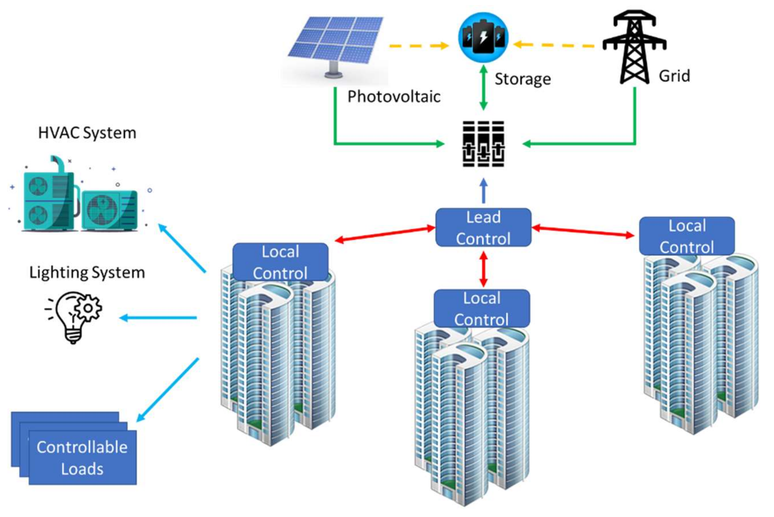
The decentralized approach places a local controller in each building, instead of having only one central controller on the building operator side. Each local controller has the capability to make decisions based on local measurements and is responsible for balancing the electricity demand and supply of the related building. Local controllers do not exchange local information with other controllers and send aggregate load data to the central controller. Hence, this approach has the additional value of securing the privacy of the occupants. The local controller negotiates the electricity supply with another local controller through the central controller. The decentralized BEMS concept has a similar concept to a hierarchy controller. Figure 3 illustrates the decentralized BEMS approach.

In practice, the local control of the decentralized approach is not only located based on the building, but may be placed based on the type of room or demographic information of the occupants. In this case, the local controller would have specialized commands and processes regarding the occupants concerned. Furthermore, a decentralized system is more stable than an identically connected centralized system; for instance, if some leaders lose their connection with other local controls, the rest of decentralized system will remain stable. In this approach, distributed data processing is considered to reduce the high requirements on the central controller (avoiding the requirements of the centralized approach).

● Distributed Approach

The growth of RESs that are installed in many places (e.g., buildings or homes) forms distributed energy resources (DER) for the microgrid. DERs are connected to provide a reliable and sustainable electricity supply. The distributed approach has drawn more and more attention due to its considerable ability to extend to a complex system for future microgrids more easily than a conventional central control approach. This approach requires that nodes have a similar capability to perform the distributed network, e.g., the node has RESs and ESSs, etc. Meanwhile, in residential buildings, the occupants do not always have their own RESs and ESSs. They depend on the electricity supplied by the building operator.

A comparison of the implementable control approaches for a BEMS is shown in

Table 1. Comparison of controller approaches implemented for a BEMS.

Type	Pros	Cons
Centralized control	Easy to implement. Easy to maintain in the case of single point failure.	Computational burden. Not easy to expand (thus not suitable for buildings). Single point of failure (highly unstable). Requires a high level of connectivity.
Decentralized control	Local information only. No need for comprehensive, two-way, high-speed communication. Without leaders, the system still includes some control cells in the buildings. Parallel computation.	Absence of communication links between agents restricts performance. Moderates scalability.

.

2.1.2. The BEMS Scenario

Considering a building operator who manages a group of residential buildings, as described in the previous section, the requirements of the BEMS are as follows:

• The building operator manages the centralized electricity generation, which consists of renewable energy sources (RESs) and electricity storage systems (ESSs) and has a connection to the grid. The BEMS needs to manage the dispatch unit of this electricity generation to support the electricity demand of the whole residential building.
• Each residential building consists of controllable loads that can be configured by the occupants to achieve the occupants’ preferences. The BEMS needs to respond and adjust the electricity management as soon as possible when the occupants input their preferences.

Following the requirements of the BEMS in residential buildings and considering the pros and cons of the control approach in Section 2.1.1, we considered the BEMS that applies the decentralized approach. The decentralized approach separates the lead controller and the local controller as depicted in Figure 3. The lead controller is placed on the building operator side, which has the responsibility to manage the electricity generation of the whole building. Therefore, in this scenario, the lead controller is responsible for managing the balance of electricity demand and electricity supply of the whole building. The lead controller applies the BEMS with load forecasting for one day ahead to predict the electricity demand of the buildings one day in advance and define the optimum dispatch unit strategy to supply the needed electricity for next day’s building operations.

The local controller is placed in each building and is responsible for managing and controlling the controllable loads inside the building. The real-time electricity usage that is recorded by the smart meter and the building state that is recorded by the sensor is sent to the lead and the local controller. However, the local controller will respond accordingly. If the real-time electricity usage is different to the prediction value from the one-day-ahead model prediction, the local controller will adjust the operation of the controllable loads and compute the one-hour ahead model prediction to adapt to the difference. The real-time data that is sent to the lead controller will be stored and used for the computation of one-day-ahead load forecasting for next day’s operations.

The decentralized approach will reduce the computation load for the lead controller, since the lead controller will focus on the one-day-ahead operations and only respond to the changes when necessary or triggered by the local controller. Changes to the real-time data and preferences at the time unit are monitored by the local controller, enabling the local controller to provide a fast response accordingly. With this approach, the computation load is distributed from the lead controller to the local controllers to perform two-level load forecasting with different time horizons.

2.2. The Framework of the Proposed Approach

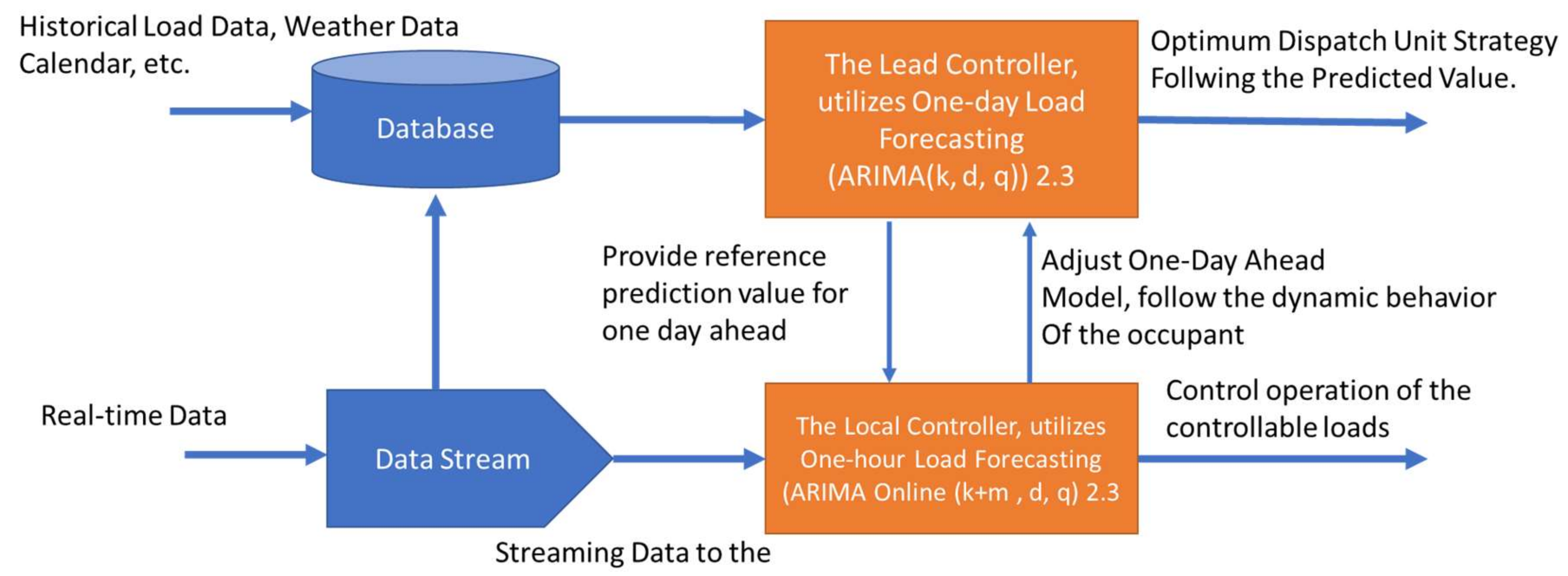
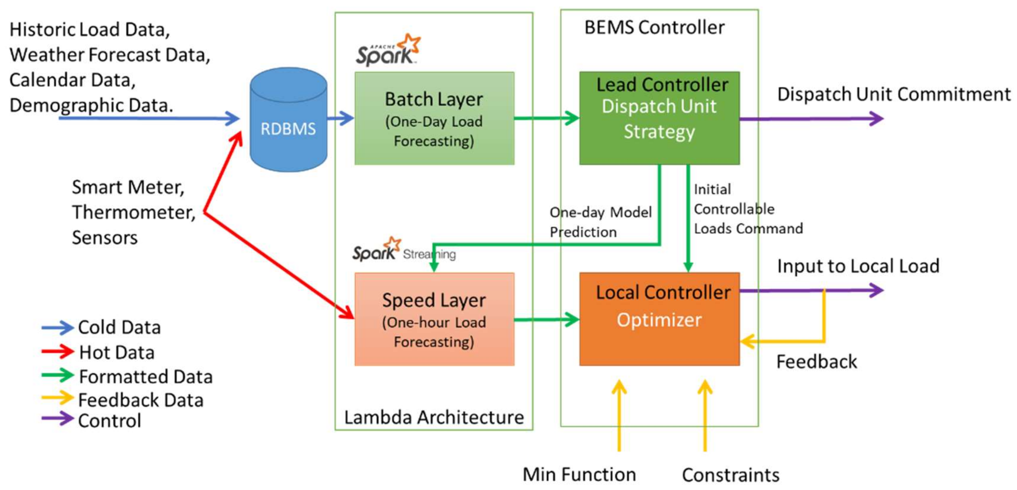
The focus of our study is a data processing architecture that reduces the processing time to produce a high accuracy load forecasting model and adapt to the dynamic behavior of the occupants. Our framework follows the decentralized approach described in Section 2.1 and defines different responsibilities between the lead controller and the local controller. Figure 4 illustrates our proposed framework.

The lead controller, which is located on the building operator side, has access to managing the electricity generation of the residential buildings. Therefore, the lead controller has the responsibility to provide an electricity supply to match the electricity demand of the whole residential building. To fulfil this responsibility, the lead controller implements one-day-ahead load forecasting techniques to predict the electricity demand on a daily basis. The lead controller utilizes the aggregate historical load data to develop one-day-ahead model predictions. One-day-ahead prediction consists of predicted electricity demand for every hour for 24 h ahead. Based on this prediction, the lead controller schedules the electricity dispatch unit for the next day to supply the electricity according to the predicted value. In the end, the lead controller distributes the one-day-ahead model prediction to each local controller as the reference to maintain and control locally controllable loads.

The local controller is located in each residential building in the domain of the building operator. The local controller is responsible for maintaining and controlling locally controllable loads inside the building. The local controller stores the real-time data on the current building state from the sensors and the current electricity consumption from the smart meter. After receiving the one-day-ahead model prediction from the lead controller, the local controller sends out the initial command to the locally controllable loads. For the next hour, the local controller evaluates the one-day-ahead model prediction based on the real-time data collected from the smart meter and the sensors. If the evaluation shows that the predicted value in the one-day-ahead model is similar to the current value, the local controller will follow the strategy of the lead controller as it is. If the evaluation shows that there are significant differences between the predicted value in the one-day-ahead model and the current value, the local controller will compute a one-hour-ahead model prediction to adjust its signal command for the next hour. With this operation, the local controller reduces the computation load of the lead controller and provide fast response to any dynamic change in the local building.

The real-time data is sent from the sensor and smart meter to the local and lead controller. The local controller will process the data as soon as it arrives, while the lead controller will hold the data and aggregate it with other data for the computation of one-day model prediction for next day.

2.3. Load Forecasting Technique

Based on the range of the prediction time, load forecasting can be classified into very short-term load forecasting (VSTLF) for a prediction range from several hours to one day, short-term load forecasting (STLF) for predictions from one day to several weeks, medium-term load forecasting (MTLF) for predictions from several weeks to three years, and long-term load forecasting (LTLF) for a prediction range from three years to many years [26]. VSTLF and STLF are mostly used for the operation and short-term planning for the BEMS, while MTLF and LTLF mostly used for budgeting, maintenance and future provision planning for the BEMS.

In this paper, we proposed two-level load forecasting where the first level will apply the STLF approach to forecast daily model predictions and the second level will apply the VSTLF approach to forecast hourly model predictions. The daily model predictions are implemented by the lead controller to define the optimum dispatch unit for daily operation, while the hourly model predictions are implemented by the local controller to adjust the control following the dynamic behavior of the occupants.

The ARIMA (Auto Regressive Integrated Moving Average) technique is one of the STLF techniques that is popular for daily model predictions for buildings based on time series models [27,28]. In this paper, we adopt the ARIMA approach that is discussed in [29]. The formula for generating model predictions based on the ARIMA is as follows:

$${\nabla }^d{X}_t={\displaystyle \sum }_{i=1}^q{\beta }_i{ϵ}_{t-i}+{\displaystyle \sum }_{i=1}^k{\alpha }_i{\nabla }^d{X}_{t-1}+{ϵ}_t,$$

(1)

where

• $X_t$ denotes the observation at time t,
• ${ϵ}_t$ denotes the zero-mean random noise term at time t,
• ${\alpha }_t$ denotes the coefficient of the autoregression (AR) model,
• ${\beta }_t$ denotes the coefficient of the moving average (MA) model, and
• ${\nabla }^d$ denotes the difference order of the $X_t$, which represents the integrate (I) model.

These parameters represent the ARIMA model, which is used for forecasting the electricity demand for one day ahead. Forecasting with ARIMA(k, d, q) is a reversion of the differential process. Suppose time series sequence $X_t$ satisfies ARIMA(k, d, q), then we can predict the d-th order differential of observation at time t + 1 as ${\nabla }^d{\tilde{X}}_t$ and then predict the observation at time t + 1 as ${\tilde{X}}_t$:

$${\tilde{X}}_t={\nabla }^d{\stackrel{{\displaystyle ˇ}}{X}}_t+{\displaystyle \sum }_{i=0}^{d-1}{\nabla }^i{X}_{t-1},$$

(2)

For the hourly model prediction, we implement the online ARIMA algorithm proposed by [29]. The online ARIMA algorithm is implemented in the local controller, which computes the online ARIMA algorithm using real-time data. The online ARIMA algorithm uses the following formula to compute the hourly model prediction for one hour ahead:

$${\tilde{X}}_t\left({\gamma }^t\right)={\displaystyle \sum }_{i=1}^{k+m}{\gamma }_i{\nabla }^d{X}_{t-1}+{\displaystyle \sum }_{i=0}^{d-1}{\nabla }^i{X}_{t-1},$$

(3)

The local controller will compute the online ARIMA algorithm based on the evaluation of the real-time value of electricity usage and the predicted value electricity usage based on the daily model prediction. If the difference is larger than the threshold, the local controller will compute the online ARIMA algorithm. Otherwise, the local controller will do nothing. This online ARIMA algorithm is needed to compute the prediction demand for one hour ahead only and does not to update the rest of the prediction based on the daily model prediction. This scenario will reduce the processing time in the local controller since it only computes what is needed.

2.4. Data Processing Architecture for the Smart Meter Data

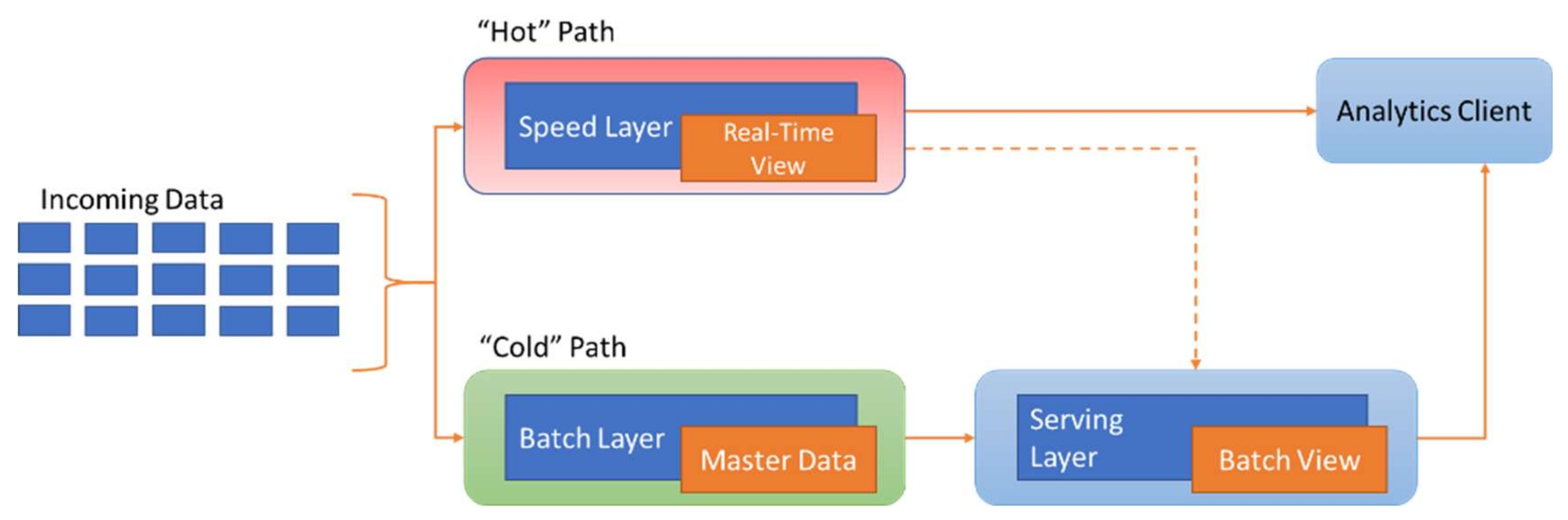
As discussed in Section 2.3, there is two level load forecasting which utilizes the smart meter data. Each level has different requirements regarding the data processing time and the velocity of data. The first level requires smart meter data that is processed one time in one forecasting period, while the second level requires real-time smart meter data that is frequently processed with limited time processing. These two types of data introduce the different requirements for the processing method. To accommodate this requirement, researchers into big data processing have introduced Lambda architecture. The Lambda architecture differentiates the data type into hot data and cold data [30].

The hot data is the data that needs to be processed immediately with a narrow time constraint. The real-time smart meter data that is processed on our second level falls into this category of data, as the data need to be processed as soon as possible to provide an immediate response to the dynamic behavior of the occupants. The cold data is the data that being processed only one time in one batch period. The data which comes after one batch processing is held and processed in the next batch. The cold data can tolerate greater latencies, since the result is not needed as soon as possible. The smart data that was processed on our first level falls into this category of data, since the first level only computes one-day ahead forecasting one time for next one day of operations. With this difference, the Lambda architecture introduces three layers to the data processing, namely the speed layer, batch layer and serving layer. Figure 5 illustrates the three layers of the Lambda architecture.

The speed layer will process the incoming data that falls into the hot data category. The speed layer processes the hot data and continuously updates the results according to the client needs. There are no historical records in the speed layer and it typically requires the fastest storage technology to analyze the hot data. Meanwhile, the incoming data which falls into the cold data category will be processed by the batch layer. The batch layer processes the cold data from the beginning until the last data before the batch job is started. The subsequent incoming data will be held and will be processed by the next batch job. This batch job processes the data at once, so the newest data will replace the predecessor data. With this concept, the batch job does not rely on incremental processing and is robust to any system failures or data loss. Each result from the speed layer and the batch layer is stored in the serving layer. This serving layer will provide the analyzed data to a client who cares about the accuracy of the data and is tolerant regarding the time latency, while for a client who cares about the data speed and is tolerant regarding less accurate data can consume the data directly from the speed layer. The Lambda architecture concept is implemented in practice with different technologies [31].

3. Proposed Data Processing Architecture Based on Lambda Architecture

In this section, we discuss the proposed data processing architecture based on Lambda architecture. We also provide the two-level load forecasting that utilizes the proposed data processing architecture in detail.

3.1. The Proposed Data Processing Architecture

Figure 6 illustrates the proposed data architecture which adopts the concept of Lambda architecture.

As shown in Figure 6, we implemented the RDBMS to store all the historical data needed by the lead controller to compute the one-day-ahead load forecasting. In our architecture, we chose the PostgreSQL as the RDBMS system. The lead controller then triggers the batch layer, which utilizes the spark technology to consume the data from the PostgreSQL and compute the one-day load forecasting using the ARIMA approach described in Section 2.3. The results from the batch layer are used by the lead controller to define the optimum dispatch unit strategy to support the predicted load demand for one day ahead. This dispatch unit strategy is sent to the electricity generator elements to schedule the electricity generation. The lead controller sends the initial controllable load command to each local controller. The local controller utilizes the initial controllable load command to initiate the operation of controllable loads in their respective residential buildings. The lead controller triggers the batch layer with the regular time interval (in this case, a one day time interval), computes and updates the one-day model prediction for next day of operations.

Spark streaming is used to process the incoming data directly from the smart meter and the sensors to evaluate the prediction value produced by the one-day-ahead model. If the evaluation shows a different result to the prediction load value and the real load value, the speed layer will compute the one-hour load forecasting using the ARIMA online approach described in Section 2.3. Otherwise, the speed layer will leave the prediction value from the one-day-ahead model prediction as it is. The local controller will use the result from the speed layer to optimize its control command.

3.2. Two-Level Load Forecasting Implementation

As shown in Figure 6, the first level of our two-level load forecasting technique is used to model the one-day-ahead load forecasting. The batch layer computes this model and it is used by the lead controller to define the optimum strategy for the dispatch unit on the electricity generation side and for the configuration of the global controllable load of the whole residential building. For this paper, we focus on how to compute the one-day-ahead load forecasting using the ARIMA approach [29] with less time computation. Spark is employed in the batch layer, which computes the ARIMA model for each iteration using all the data stored in the PostgreSQL database. The result of this computation is the value of ${\alpha }_t$, ${\beta }_t$, ${\nabla }^d$, and ${ϵ}_t$, which represents the ARIMA model. Algorithm 1 summarizes step-by-step our first-level load forecasting, which is the implementation of the ARIMA function for the historical load data. The values ${\alpha }_t$, ${\beta }_t$, ${\nabla }^d$, and ${ϵ}_t$ will be saved and used by the speed layer.

Algorithm 1. One-day-ahead model prediction for the first level.

1: function FirstLevel(TimeSeriesCollection TS)

2:  M ← {}

3:  Input: parameter k, d, q

4:  co-mpute ${\mathbf{\alpha }}_{\mathit{t}}$, ${\mathbf{\beta }}_{\mathit{t}}$, ${\mathbf{\nabla }}^{\mathit{d}}$, and ${\mathbf{ϵ}}_{\mathit{t}}$ using ARIMA(k,d,q)(TS)

5:  input ${\mathbf{\alpha }}_{\mathit{t}}$, ${\mathbf{\beta }}_{\mathit{t}}$, ${\mathbf{\nabla }}^{\mathit{d}}$, and ${\mathbf{ϵ}}_{\mathit{t}}$ into M

6:  return M

The second level of our two-level load forecasting method is deployed in the speed layer. Algorithm 2 describes the process of the second level, which adjusts the one-day-ahead model and produces a one-hour-ahead model if there is the difference between the actual load usage with the prediction value from the one-day-ahead model forecast.

Algorithm 2. One-hour-ahead model prediction for the second level.

1: N = 24 (h)

2: function SecondLevel(CurrentLoadUsageCollection L, PredictModel M)

3:  predict $\stackrel{{\displaystyle ˇ}}{{\mathit{X}}_{\mathit{t}}}$ using M (from first-level)

4:  compute ${\mathit{X}}_{\mathit{t}}$ as the average of CurrentLoadUsageCollection L at the end of each time unit.

5:  if $\stackrel{{\displaystyle ˇ}}{{\mathit{X}}_{\mathit{t}}}$ = ${\mathit{X}}_{\mathit{t}}$

6:    N = N − 1 and do step 3

7:  else

8:    Compute OnlineARIMA Model for N + 1 to obtain ${\mathit{\alpha }}_{\mathit{t}\mathbf{+}\mathbf{1}}$, ${\mathit{\beta }}_{\mathit{t}\mathbf{+}\mathbf{1}}$, ${\mathbf{\nabla }}^{\mathit{d}}$

9:    Predict $\stackrel{{\displaystyle ˇ}}{{\mathit{X}}_{\mathit{t}\mathbf{+}\mathbf{1}}}$ using parameter from step 8 and do step 4.

10:    Adjust control command

11: Until N = 0

We implemented the algorithm to process real-time data using Spark Streaming. All real-time data was processed directly in Spark Streaming to detect the difference between the real value and the predicted value. The real-time data was also stored in the PostgreSQL for the next batch job in the batch layer.

4. Evaluation

In this section, we will evaluate the performance of our proposed data processing architecture and two-level load forecasting method in terms of cost reduction and computation time. The accuracy of the model prediction can be transformed into the cost if there is a mismatch between the prediction value and the real value. Then we will use this cost parameter to measure the effectiveness of our approach to reduce the cost caused by the accuracy of the model prediction. We deploy the scenario for cost reduction as follows: (1) model prediction without optimization; and (2) model prediction with optimization as in the two-level load forecasting method. Comparing the cost reduction from these two scenarios will show the advantages of the proposed two-level load forecasting method.

The design of the Lambda-like data processing architecture is intended to reduce the computation time for developing the model prediction and provide the control command as soon as possible in order to respond to the dynamic changes of the occupants. The processed data is the historical load data in the Time Series format. We measure the computation time needed to process the variation number of the Time Series data with the scenarios as follows: process all the smart meter data in the lead controller, process smart meter data with different layer processing and the centralized approach, and process smart meter data with different layer processing and the decentralized approach.

For this evaluation, we used the real dataset from [32], which contains the electricity consumption readings for 5567 London households that are part of the UK power network. The data was collected from November 2011 to February 2014. However, we only considered the data set from 2012 and 2013, which has complete data. We divided the dataset into a training set and a test set. The training set was used to develop the model prediction, and the test set was used as the ground truth to compute the accuracy of our model.

4.1. Cost Reduction

The cost that resulted in the accuracy of the model prediction can be calculated using the following formula:

$$Cos{t}_{acc}={\displaystyle {\displaystyle \sum }_{t=1}^T}\left|L{P}_t-L{R}_t\right|\times ElectricityCostper kW{h}_t,$$

(4)

The absolute value of the difference between LP and LR is to define the total cost caused by the load forecasting accuracy. However, in the real situation, the difference between LP and LR at the time may have had a negative or positive value, which must have the following meaning:

• A negative value means that the prediction load was less than the real load. In this case, the building operator needs to supply more electricity, which means additional cost.
• A positive value means that the prediction load was greater than the real load. In this case, the building operator spent more than needed.

We assumed the price of the electricity using the time of use schema illustrated in

Table 2. The price assumption of electricity following the time of use (ToU) schema [33].

Day of the Week	Time of Day	ToU Period	ToU Price
Weekend & Holidays:	All day	Off-peak	$0.065 per kWh
Weekdays:	7:00 a.m. to 11:00 a.m.	On-peak	$0.132 per kWh
	11:00 a.m. to 5:00 p.m.	Mid-peak	$0.095 per kWh
	5:00 p.m. to 7:00 p.m.	On-peak	$0.132 per kWh
	7:00 p.m. to 7:00 a.m.	Off-peak	$0.065 per kWh

.

The two-level load forecasting method can be used to optimize the Cost_acc for each household in a group of residential houses or the whole Cost of the residential buildings. In this evaluation, we calculate the Cost_acc that applied to one household. Scenario 1 is the load forecasting using one-day model prediction without any optimization, and Scenario 2 is the load forecasting using one-day model prediction using optimization in the second level to adapt to the dynamic behavior of the occupant.

4.1.1. Scenario 1: Model Prediction without Optimization

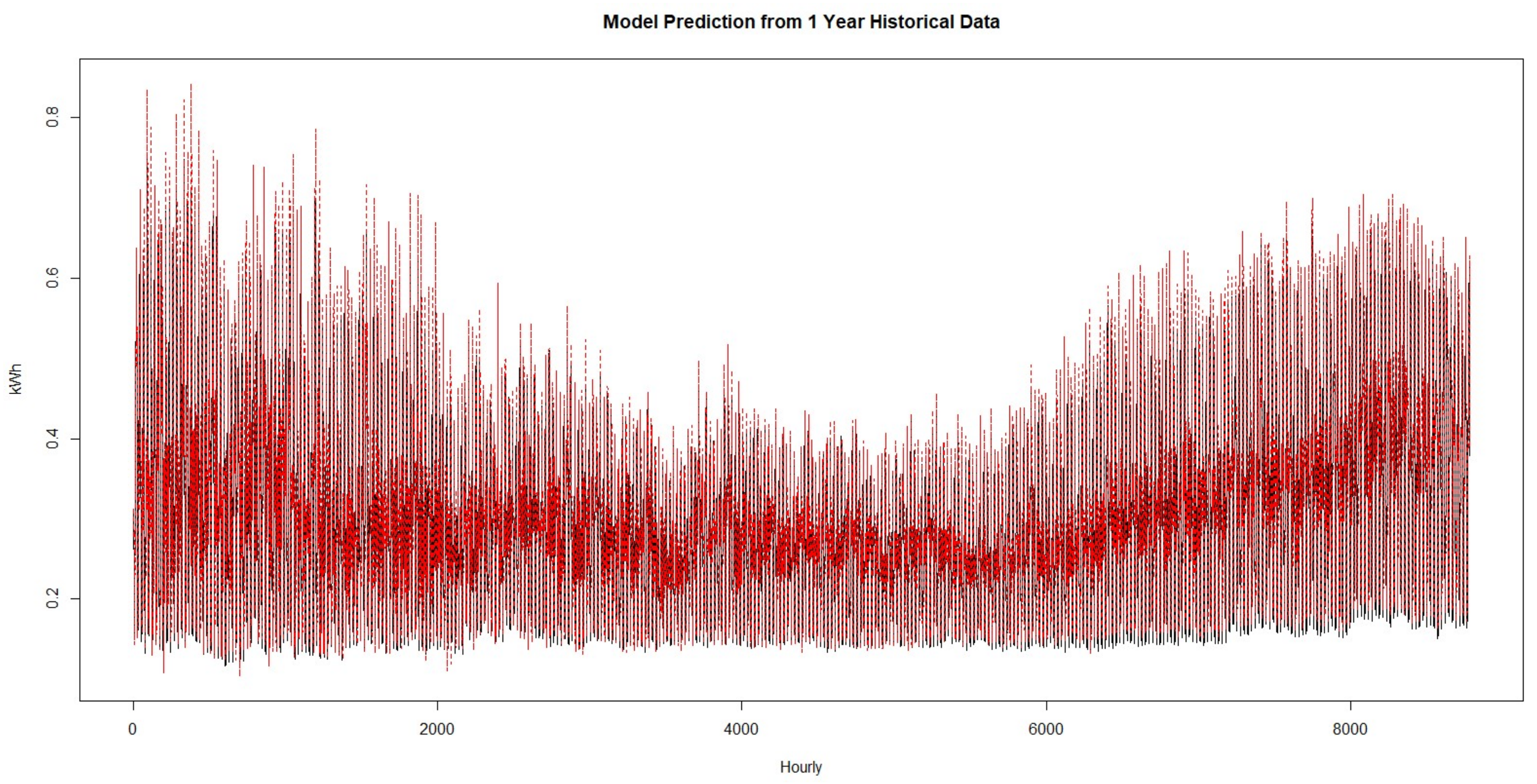
In this scenario, we computed the one-day-ahead model prediction using aggregate data from the previous one year. We used the model directly to predict the one-day-ahead electricity demand. We predicted the one-day-ahead electricity demand for the whole building operation and the individual user. Figure 7 shows the model prediction developed using the previous year’s historical load data.

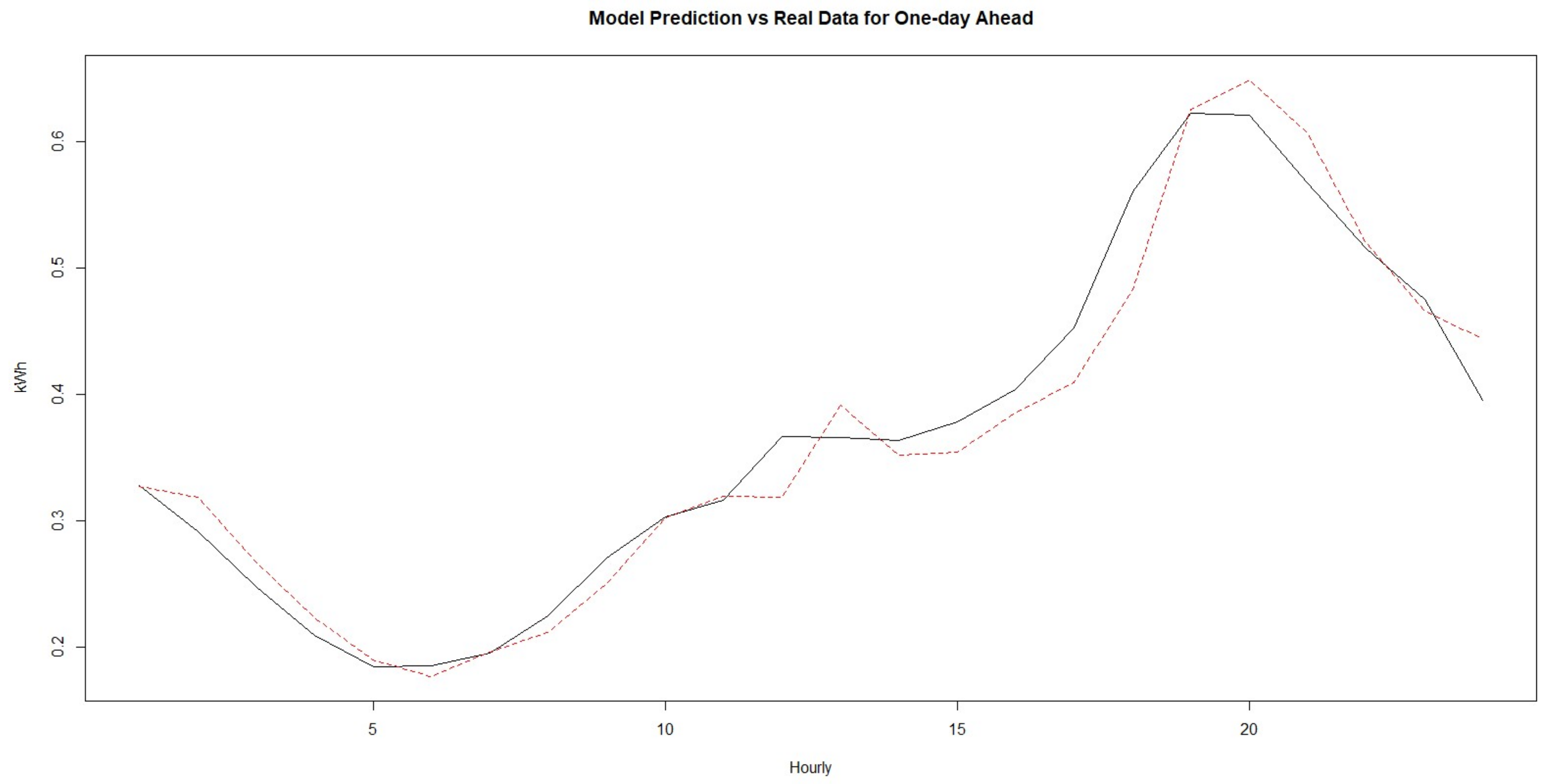
We can see from Figure 7 that the model prediction has a similar value as the real data. The usage of the model prediction directly to predict the one-day-ahead electricity demand will provide the result showed in Figure 8.

We can see from Figure 8 that the prediction value is not quite the same as for the real data. With the price assumption from Table 2, the cost of the prediction seen in Figure 8 was calculated using Equation (4), and the result is

$$Cos{t}_{acc}={\displaystyle \sum }_{t=1}^{24\mathrm{h}}\left|L{P}_t-L{R}_t\right|\times ElectricityCostperkW{h}_t= \$0.246/\mathrm{kWh}$$

(5)

4.1.2. Scenario 2: Model Prediction with Optimization

Following our proposed two-level load forecasting, the one-day-ahead model prediction was being optimized to produce a one-hour ahead model prediction using the real-time data from the smart meter. The result of this optimization is illustrated in Figure 9.

From Figure 9, we can see that the second level of our proposed load forecasting optimized a prediction value similar to the real value. The cost of the optimization accuracy is:

$$Cos{t}_{acc}={\displaystyle \sum }_{t=1}^{24\mathrm{h}}\left|L{P}_t-L{R}_t\right|\times ElectricityCostperkW{h}_t= \$0.228/\mathrm{kWh}$$

(6)

Comparing the Cost_acc value from Scenario 2 and Scenario 1 shows that the two-level load forecasting reduced the Cost by around 7%. If the reduction is accumulated with other occupants in the residential building, the two-level load forecasting will help the building operator to save significantly on the electricity cost.

4.2. Computation Time Analysis

We analyzed the computation time needed to compute the model prediction with the scenarios as follows: process all the smart meter data in the lead controller, process smart meter data with different layer processing and the centralized approach, and process smart meter data with different layer processing and the decentralized approach. The dataset used in this scenario was the hourly smart meter data from 2012 and 2013. This dataset resulted in around 3.6 million Time Series data in form of 24-h data points for every day and every household. The example of the Time Series is shown in Figure 1 for the individual data, which consists of seven Time Series data coming from seven days and one household. 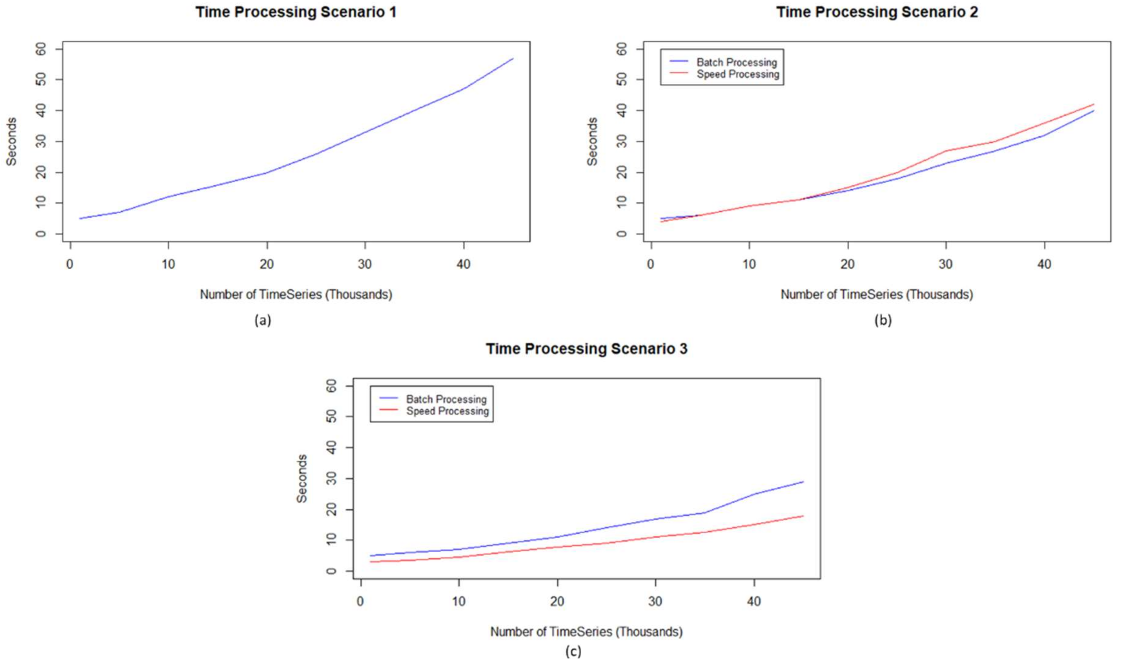Figure 10 illustrates the computation time for each scenario.

Figure 10a shows the computation time for one controller under the centralized approach, which handles the computation for all the smart meter data. The computation time in this scenario depends on the number of time series that are being processed by the central controller. The increasing number of time series, caused by the increasing number of smart data, will increase the computation time of the central controller.

Figure 10b shows the computation time for a controller that implements different layer processing in one machine. In this scenario, the computation time of the speed layer is slightly longer than the batch layer. This is because this type of machine must schedule the speed of processing following the batch layer. The optimum scheduling of processing will improve the performance of this scenario.

In Figure 10c, the batch layer and the speed layer are in a different machine, following the concept of a decentralized approach. In this scenario, the computation time for each layer is independent. The computation time in the batch layer, which is located in the lead controller, will increase following the number of time series data. This is the apparent pattern, but the computation time is lower than for other scenarios. The speed layer has a low computation time since it does not have to wait for batch processing. Also, speed layer processing is not as heavy as batch layer processing, since the time series computation does not request the historic data. This scenario has thus shown that our approach has the best performance compared to the other scenarios.

5. Related Work

Several previous studies have proposed various load forecasting techniques that can be used by the BEMS to address the uncertainty problem. These load forecasting techniques develop the model prediction using smart meter data in the form of the aggregation of data or individual/real-time data. Each form of smart meter data gives different benefit to the BEMS when addressing the uncertainty problem. The aggregation form of smart meter data is utilized by the authors in [3,10]. The authors in [3] apply the combination of stacked autoencoders (SAEs) and an extreme learning machine (ELM) to develop model predictions using aggregation data. The historical load data in this paper was collected every 15 min from one retail building in Fremont, CA, and was pre-processed to aggregate the data into 30 and 60 min data. This historical data was then used by the proposed technique to predict the electricity usage for a certain time ahead. The authors in [10] developed a load forecasting technique using support vector regression (SVR) and applied it to a dataset collected from a multi-family residential building in New York City. This technique was developed to predict the energy consumption of the building with less input data. The proposed technique was developed based on the machine learning technique to infer the complex relationship between consumption and influencing variables (e.g., weather data and previous consumption).

The individual/real-time form of smart meter data was utilized by the authors in [29,34]. The authors in [34] proposed a load forecasting technique based on an artificial neural network (ANN) to develop model predictions using real-time data from a smart meter. In this work, the proposed technique was used to predict the energy consumption of the HVAC system of a hotel building in Madrid, Spain. This work considered the HVAC system as the case study because it consumes a significant amount of energy in the hotel building. Also, the control mechanism of the HVAC system needed to be optimized to the running cycle of the HVAC system. Therefore, a real-time load forecasting technique was needed to address the optimization problem of the HVAC system. The ANN technique was used in this work due to its fault-tolerant, noise-immune and robust nature. With these characteristics, an ANN can easily model noisy data and is appropriate to analyze real-time data from a smart meter. The authors in [29] proposed a load forecasting technique to analyze the real-time data from a smart meter using a modification of the ARIMA (autoregressive integrated moving average) technique. The smart meter data, which was arranged based on the timestamp, was able to form time-series data on the energy consumption. The original ARIMA utilized this time-series data to build a model prediction of electricity consumption. However, the original ARIMA can only be used to analyze historical load data. In this work, the authors modify the formula of ARIMA to adopt real-time, time-series data from a smart meter. The result is the Online ARIMA technique, which can be used to predict very short load forecasting (e.g., one-h ahead) using real-time data.

The load forecasting technique that was described above handles the form of the smart meter data separately. Although each technique showed promising results regarding the model’s prediction accuracy, there are shortcomings when implementing the BEMS. The load forecasting technique that utilizes aggregation data from a smart meter enables the BEMS to know the electricity consumption in advance and design a strategy according to the model prediction. However, this technique is vulnerable to the uncertainty problems of the BEMS, which produce a mismatch of the measured data and the predicted data. Meanwhile, the load forecasting technique that utilizes the individual/real-time data from a smart meter enables the BEMS to adapt with according to the uncertainty problem over time. However, this technique can only be used by the BEMS to be reactive to dynamic changes. The BEMS cannot design a strategy in advance to maintain the balance of the electricity supply and electricity demand of a building. To address this problem, there are studies that try to combine the process of the aggregation form and individual/real-time form of smart meter data [22,35,36,37]. The proposed technique in this study applies two-level load forecasting, where the first level utilizes the aggregation data for short-term load forecasting (e.g., one day ahead) and the second level utilizes the individual/real-time data for very-short-term load forecasting (e.g., one hour ahead).

The authors in [35] proposed a hierarchical control structure based on model predictive control (MPC), where the structure consists of two anticipated layers: a scheduling MPC (S-MPC) with a long-term horizon and a piloting MPC (P-MPC) dealing with a short term-horizon. The authors consider the fluctuation of energy tariffs and the available power that can be supplied by the grid market. The authors in [22] proposed a strategy for the BEMS that consists of prediction, long-term scheduling, and real-time control (RTC). As with the previous study, the authors in this study considered the fluctuation tariff, as well as external data to develop the model prediction for the long-term horizon. This model prediction is used by the long-term scheduling part to define the optimum scheduling dispatch unit. The RTC is used to adapt to the dynamic changes of electricity usage in real-time and adjust the long-term model prediction for (N-1) hours. This study considers the electricity flow in a building where renewable energy sources are involved. The authors in [36] propose a cost-for-deviation (CfD) retail-pricing schema that is designed to reduce the demand uncertainty of individual customers or communities. The authors expand their approach to not only apply to one building, but also to two or more buildings in a community. The approach in this study consists of a day-ahead planning layer and a real-time tracking optimization problem layer. The authors in [37] propose a two-stage energy management system (EMS) that is suitable for small-scale, grid-connected electrical systems. The proposed approach is designed to reduce the demand uncertainty and the electricity cost for the end users, at the same time. The first stage of the proposed approach utilizes the ANN technique to forecast the renewable generation and load demand. The second stage is used to consider user preferences and produce the command for the hardware controller while maintaining the balance of the electricity supply and demand of the building.

The two-level load forecasting discussed above enabled the BEMS to define the optimum strategy for long-term operation and to adapt dynamically to addressing the uncertainty problem. However, these studies have not yet considered the data processing of the smart meter data. Efficient data processing is needed to reduce the processing time of the load forecasting technique while still achieving reasonable accuracy. Our paper addresses this problem by proposing a Lambda-based data processing architecture, which separates the layers to process the aggregation data as cold data and the individual/real-time data as hot data. In

Table 3. Features of the proposed and recent works.

No.	Papers	Aggregation/Individual Data	Centralized/Decentralized	Two-Level Appraoch	Building Type	Methods	Cost Saving	Data Processing
1	[3]	Aggregation	Centralized	NA	Retail building	ExtremeSAE	NA	No
2	[10]	Aggregation	Centralized	NA	Residential Building	SVR	NA	No
3	[34]	Aggregation	Centralized	NA	Hotel Building	ANN	NA	No
4	[29]	Individual	Centralized	NA	Synthetic Data	Online ARIMA	NA	No
5	[35]	Both	Centralized	Yes	Residential Building	NA	NA	No
6	[22]	Both	Centralized	Yes	Commercial Building	ARIMA	10–20%	No
7	[36]	Both	Centralized	Yes	Office Building	ANN	14.3%	No
8	[37]	Both	Centralized	Yes	Residential Building	ANN	10.35%	No
9	Our Proposed System	Both	Decentralized	Yes	Residential Building	ARIMA/Online ARIMA	7%	Lambda-based

, we show the comparison of our approach with that of relevant works on load forecasting techniques for BEMSs.

6. Conclusions

The two-level load forecasting technique promises to address the uncertainty problem in the BEMS. This study aimed to evaluate a data processing architecture that supports the computation requirements and time constraints of the two-level load forecasting technique. This study proposed a data processing architecture based on Lambda architecture that separates the layers to process aggregated and individual/real-time data from a smart meter separately. The first level of the two-level load forecasting technique utilizes the batch layer to process the aggregation data once at the horizon time and to produce a one-day-ahead model prediction. This one-day-ahead model prediction is used by the BEMS to predict the electricity demand for the next day so that the BEMS can formulate an effective dispatch unit strategy for the day’s building operations. The second level of the two-level load forecasting technique utilizes the speed layer to process the individual/real-time data. This speed layer compares the measured value with the predicted value from the first level. If the values do not match, the speed layer will compute the one-hour-ahead model prediction to adjust the electrical element operation and the one-day-ahead model prediction accordingly. With this method, our approach enables the BEMS to address the uncertainty problem more effectively and to reduce the time processing of the two-level load forecasting.

The main difference of our approach compared to previous work is the location of the first and second level of the two-level load forecasting. The previous works locate the first level and second level of the two-level load forecasting method in the same machine. In this study, we adopt the decentralized control approach, where the BEMS separates the lead controller and the local controller. The first level and the batch layer of our Lambda-based data processing is in the lead controller. The second level and the speed layer of our Lambda-based data processing is in the local controller. With this approach, we expect to reduce the computation load of each controller and accelerate the respond of the BEMS to address the dynamic behavior of the occupant.

In this study, we applied the ARIMA technique for the first level and the online ARIMA technique for the second level. We evaluated our approach using a real dataset for residential buildings. The evaluation showed that our approach reduced the cost of the load forecasting by around 7% and had the lowest computation time. This result shows the applicability of our approach for the BEMS. In this study, we considered the electricity data of a BEMS where this data is widely available and used in recent load forecasting research. However, we argue that our approach is applicable to other energy sources for BEMSs. In the future, we plan to evaluate our data processing architecture using other load forecasting techniques such as ANN and SVM. We also plan to deploy our approach to the cloud, moving towards the BEMS as a service.