Article

Calculation of Equivalent Resistance for Ground Wires Twined with Armor Rods in Contact Terminals

1
School of Electric Power, South China University of Technology, Guangzhou 510640, China
2
School of Mechanical & Automotive Engineering, South China University of Technology, Guangzhou 510640, China
*
Author to whom correspondence should be addressed.
Energies 2018, 11(4), 737; https://doi.org/10.3390/en11040737
Submission received: 16 February 2018 / Revised: 19 March 2018 / Accepted: 22 March 2018 / Published: 24 March 2018
(This article belongs to the Section F: Electrical Engineering)

Abstract

:
Ground wire breakage accidents can destroy the stable operation of overhead lines. The excessive temperature increase arising from the contact resistance between the ground wire and armor rod in the contact terminal is one of the main reasons causing the breakage of ground wires. Therefore, it is necessary to calculate the equivalent resistance for ground wires twined with armor rods in contact terminals. According to the actual distribution characteristics of the contact points in the contact terminal, a three-dimensional electromagnetic field simulation model of the contact terminal was established. Based on the model, the current distribution in the contact terminal was obtained. Subsequently, the equivalent resistance of a ground wire twined with the armor rod in the contact terminal was calculated. The effects of the factors influencing the equivalent resistance were also discussed. The corresponding verification experiments were conducted on a real ground wire on a contact terminal. The measurement results of the equivalent resistance for the armor rod segment showed good agreement with the electromagnetic modeling results.

1. Introduction

Usually, overhead ground wires are erected over high-voltage electric transmission lines to protect the lines against direct lightning strikes. Particularly during the thunderstorm season, the presence of ground wires can effectively guarantee the safety and stable operation of the overhead lines [1,2,3,4,5,6]. However, when short circuit accidents occur in the overhead lines, the power frequency short-circuit current may flow through the ground wire. Under the action of the power frequency short-circuit current, the temperature of ground wire may increase drastically within a short time; and as the temperature reaches the fusion point, cases of wire breakage may occur. To ensure the safe operation of the ground wire, it is necessary to accurately calculate the temperature of the ground wire. The majority of previous reports on the temperature field calculation of ground wire have used the ontology of ground wire as the research object [4,5,6]. The authors in [7] pointed out that in the contact terminal, contact resistance existed between the ground wire and armor rod. Thus, the equivalent resistance of the ground wire twined with armor rod in the contact terminal is larger than that of the ontology of the ground wire with the same length, which results in a higher temperature rise in the contact terminal [8]. Therefore, investigation into the calculation of equivalent resistance for ground wires twined with armor rods in contact terminals is significant when evaluating the possibility of ground wire breakage.
In the investigation of electrical contact, the theory at the microscopic level generally accepted by researchers currently is the constriction resistance theory proposed by Holm [9]. Based on [9], Greenwood established the contact resistance calculation formula considering the interaction of multiple contact points subsequently [10], and Kogut proposed a mathematical model for the calculation of the contact resistance based on the rough contact surface [11]. However, the above studies failed to establish contact with the macro level, so they were difficult to use in practical applications. Moreover, with the development of computer technology, finite element analysis (FEA) methods have gradually been used in the research on electric contact. In the application of FEA methods, the equivalent treatment of contact interface has always proved difficult. Several researchers have applied a layer of film with a constant thickness onto the contact interface, and the different contact conditions were simulated by varying the material properties of film [12,13,14]. In addition, several studies established tiny contact points models on the contact interface to simulate the contact conditions [15,16,17,18,19]. The most widely used contact points models were the conductive bridge model and the coupled contact interface model.
Currently, only a few studies have investigated the effects of relevant geometric parameters of the contact points model on the contact resistance [18,19]. In [18], the case of multiple contact points was not considered, and only a conductive bridge was employed to achieve electric connection of the contact interface. The simulation model containing multiple conductive bridges was established in [19]; however, for the model in [19], the distribution characteristic of conductive bridges did not conform to the actual distribution characteristic of contact points. Therefore, the above models could not accurately calculate the actual current distribution on the contact interface.
In this paper, the cylindrical conductive bridges model was adopted to simulate the contact points between the ground wire and the armor rod near the contact surface. Combined with the actual distribution characteristic of the contact points, a three-dimensional electromagnetic field simulation model based on the multiple contact points model (referred to as “3D-EM model”) of the contact terminal was established. Based on the 3D-EM model of the contact terminal, the distribution characteristic of current nearby the contact surface was analyzed, and the equivalent resistance of the ground wire segment twined with the armor rod (referred to as “armor rod segment”) in the contact terminal was calculated. Subsequently, the effects of the relative permeability of steel and the stranding parameters of ground wire and armor rod on the equivalent resistance of the armor rod segment were discussed. The steady-state temperature rise experiments of the contact terminal and the equivalent resistance measuring experiments for the armor rod segment were conducted. According to the coupling of the electromagnetic field and the thermal field, a method for determining the conductive bridge radius r was proposed, which was based on the criterion of the minimum sum of squared error between the simulation and experimental results of contact terminal surface temperature. The experimental results of the equivalent resistance for the armor rod segment verified the accuracy of the 3D-EM model of the contact terminal.
The remainder of the paper is organized as follows: Section 2 presents the equivalent treatment method for the contact points in the FEA model of the contact terminal. Section 3 presents the 3D-EM model of the contact terminal. Section 4 presents the method for the experimental verification of the 3D-EM model. Section 5 presents the analysis of factors affecting the equivalent resistance of the armor rod segment. The conclusions are shown in Section 6.

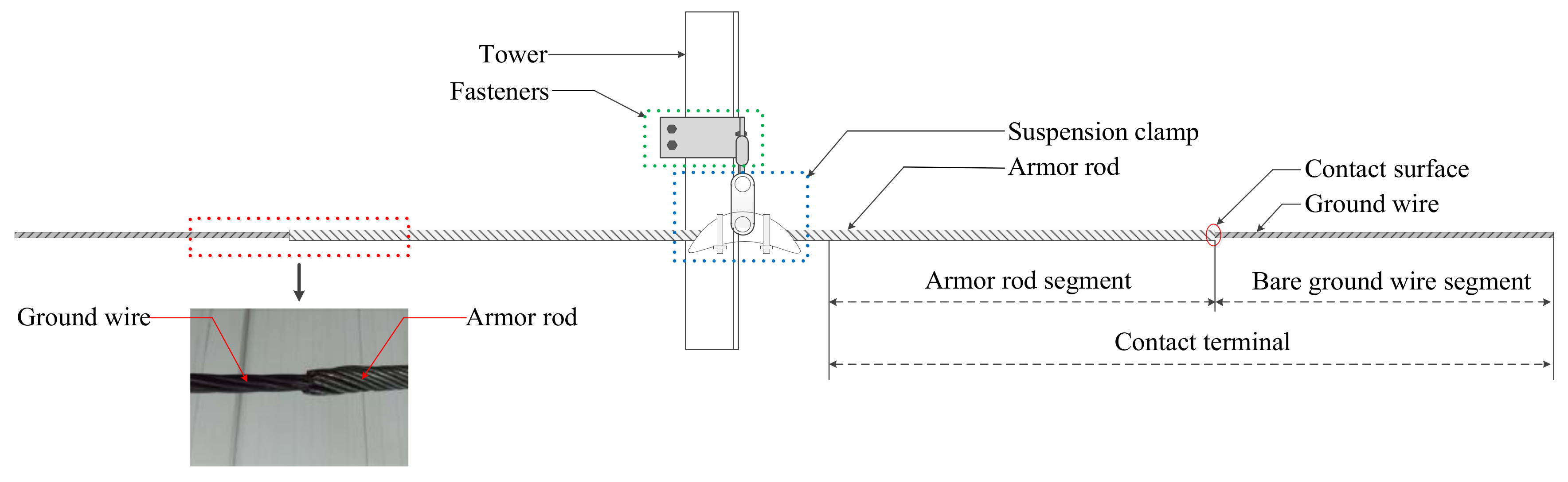
2. Multiple Contact Points Model of the Contact Terminal Consisting of Ground Wire and Armor Rod

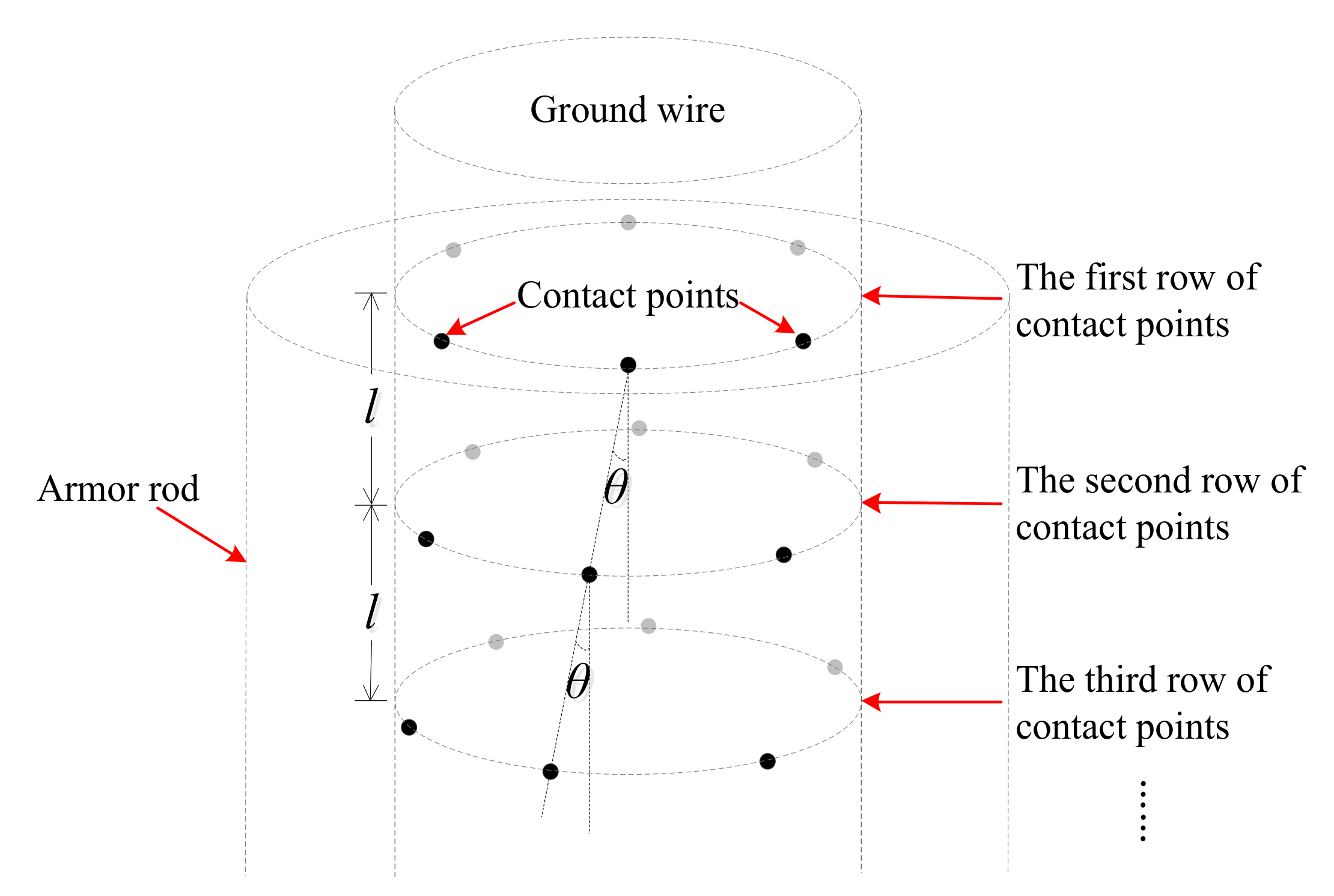
2.1. Spatial Distribution of the Contact Points between the Ground Wire and the Armor Rod

To improve the shock resistance capacity of the steel-stranded overhead ground wire at the site of the suspension clamp, a layer of armor rod stranded by 12 strands of steel wire is usually twined around the ground wire [20], as shown in Figure 1. The authors in [7] pointed out that when alternating current (AC) flowed from the ground wire segment without twined armor rod (referred to as “bare ground wire segment”) into the armor rod segment, current diffusion occurred in the contact terminal consisting of armor rod and ground wire (referred to as “contact terminal”) due to the skin effect. To obtain the current distribution in the contact terminal, it is necessary to investigate the spatial distribution characteristics of the contact points between the ground wire and the armor rod.
For the radial cross section of the armor rod segment, it can be observed that a relative rotation occurs between different layers with changes in axial position. The relative rotation angle between the different layers depends on the stranding directions and the lay lengths of different layers. In the case where the ground wire and the armor rod are stranded in the same direction and the lay length of the ground wire is shorter than that of the armor rod, the variation process of the contact points distribution at the radial cross section of the armor rod segment with a change in the axial position is obtained, as shown in Figure 2.
Based on the structural characteristics of the ground wire and armor rod, the contact points between the ground wire and the armor rod are located at the points of tangency between the armor rod layer and the outermost layer of the ground wire. An example of the radial cross section of the armor rod segment with contact points (i.e. case 1) is shown in Figure 2a. Due to the difference of the lay length between the armor rod layer and the outermost layer of the ground wire, relative displacement occurs between the two layers as the axial position changes. Then, a transitional stage at which there is no contact point between the armor rod layer and the outermost layer of the ground wire (as shown in Figure 2b) exists before the appearance of the next radial cross section of the armor rod segment with contact points (case 2 in Figure 2c).
Combined with the definition of the lay length, for the same parts at different radial cross sections, the relative rotation angle between them is proportional to their axial distance. Thus, the distance from a radial cross section of the armor rod segment with contact points to the next radial cross section of the armor rod segment with contact points is a constant, defined as l in Figure 3. l can be obtained by Equation (1):
{ l 1 = 360 / 12 | 360 / s 1 360 / s 2 | = s 1 s 2 12 | s 1 s 2 | l 2 = 360 / 12 360 / s 1 + 360 / s 2 = s 1 s 2 12 ( s 1 + s 2 )
In Equation (1), l1 and l2 are the axial distances between two adjacent radial cross sections of the armor rod segment with contact points when the stranding directions of the armor rod and the outermost layer of the ground wire are identical and opposite, respectively; s1 and s2 are the lay length of the outermost layer of the ground wire and the lay length of the armor rod, respectively.
To further explain the characteristics of spatial distribution of the contact points between the ground wire and the armor rod, θ is introduced to signify the rotation angle of the adjacent two contact points on the same strand of the one with smaller lay length between the armor rod and the outmost layer of the ground wire, as shown in Figure 3. θ can be computed according to Equation (2):
{ θ 1 = 360 l 2 s min = 30 s 1 s 2 | s 1 s 2 | s min θ 2 = 360 l 1 s min = 30 s 1 s 2 ( s 1 + s 2 ) s min
In Equation (2), θ1 and θ2 are the rotation angles of the adjacent two contact points on the same strand of the armor rod when the stranding directions of the outermost layer of the ground wire and the armor rod are identical and opposite, respectively. smin is the minimum value between s1 and s2, i.e.,:
s min = min ( s 1 , s 2 )

2.2. Equivalent Treatment of the Contact Points between the Ground Wire and the Armor Rod in the FEA Model

When establishing the simulation model of the contact terminal, the geometric models of the ground wire and the armor rod are simplified as follows: the stranded ground wire is substituted with a cylinder of the same outer diameter, whereas the stranded armor rod is substituted with a circular tube with an outer diameter equal to that of the armor rod segment and an inner diameter 2H larger than the outer diameter of the ground wire [21,22]. To ensure that the current distribution in the simulation model is in accordance with the actual current distribution in the contact terminal, a cylindrical conductive bridge model with the height of H is used to simulate the conductive contact points between the external surface of the ground wire and the internal surface of the armor rod. It is assumed that the material of the cylindrical conductive bridge model is the same as the material of the steel, and H is 0.1 mm [17]. Different contact cases between the ground wire and the armor rod can be simulated by changing the cylindrical conductive bridge radius r. The non-contact part between the external surface of the ground wire and the internal surface of the armor rod is filled with a non-conductive air gap. Thus, based on the spatial distribution characteristics of the contact points between the ground wire and the armor rod and the above simplification, a multiple contact points simulation model of the contact terminal can be established. The radial cross section with contact points of the armor rod segment in the model is shown in Figure 4.
As shown in Figure 4, for the multiple contact points simulation model, the external surface of the ground wire and the internal surface of the armor rod are connected by a series of cylindrical conductive bridges with the same distribution characteristics as the actual contact points, whereas the non-contact part does not influence the analysis of the contact interface between the ground wire and the armor rod. Thus, the simplification of the geometric models of the ground wire and the armor rod does not influence the electric contact properties of the contact terminal; moreover, it can even reduce the workload of geometric modeling for the contact terminal.

3. FEA Computation of the Electromagnetic Field for the Contact Terminal Based on the Multiple Contact Points Model

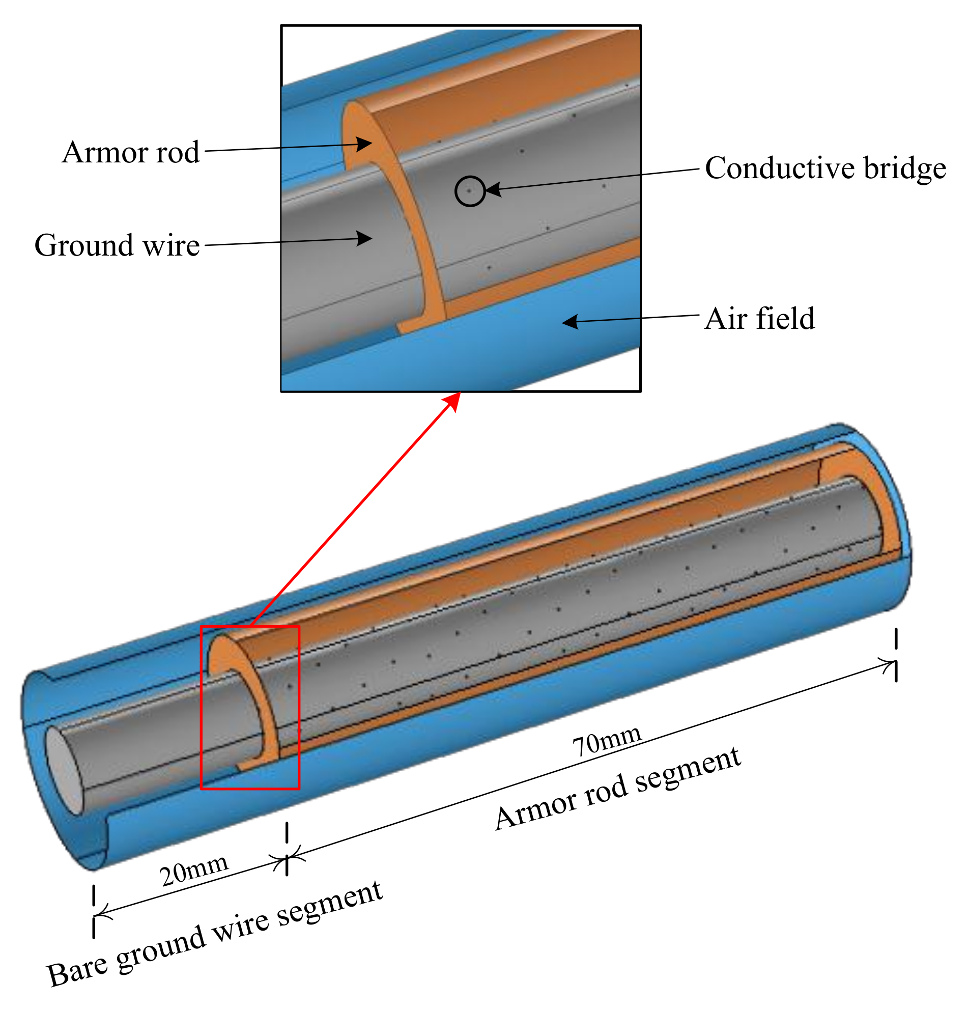
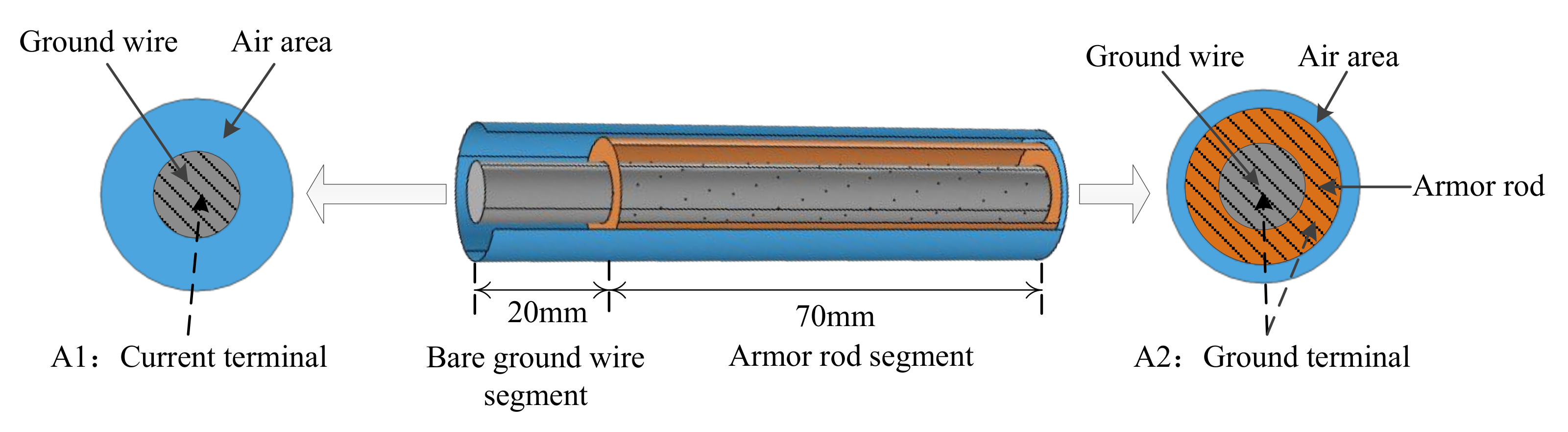
3.1. Geometric Model of the Contact Terminal

A 50 mm2 ground wire and the corresponding armor rod were taken as the example to investigate the electric contact properties of the contact terminal. Based on the equivalent treatment method for the conductive contact points in Section 2.2, the 3D-EM model of the contact terminal was established in COMSOL, and its geometric model is shown in Figure 5.
In Figure 5, the air field wrapped around the ground wire and armor rod is equivalent to a hollow coaxial cylinder with an axial length the same as the ground wire, which facilitates the setting of electromagnetic field boundary conditions in the 3D-EM model. Furthermore, the simulation results show that varying the external diameter of the equivalent cylinder of the air domain has no influence on the current distribution calculation results of the 3D-EM model. Thus, in this paper, the external diameter of the equivalent cylinder of the air field was set to 20 mm. Important geometric parameters of the 3D-EM model of the contact terminal are shown in Table 1.

3.2. The Physical Parameters and the Boundary Conditions of the Model

The material of the ground wire and the armor rod was steel, and some of the physical parameters of the steel are shown in Table 2.
In Table 2, the relative permeability of steel generally ranged from 300 to 4000 due to different carbon content and can be significantly influenced by the manufacturing techniques used [23]. Combined with the computational formula of the ratio of the direct current (DC) resistance to the AC resistance (i.e., Equation (4)) and the computational formula of skin depth (i.e., Equation (5)), the relative permeability of steel can be obtained:
R 2 R 1 = S 1 S 2 = r g 2 r g 2 ( r g d ) 2
In Equation (4), R1 and R2 are the DC resistance and the power frequency AC resistance of the conductor, respectively; S1 and S2 are the equivalent sectional areas of the conductor through by the direct current and the power alternating current, respectively; and rg is the radius of the ground wire; d is the skin depth of steel under the power frequency of 50 Hz, which can be computed according to Equation (5). In Equation (5), ω is the angular frequency; μr and μ0 are the relative permeability of steel and the permeability of vacuum, respectively; and γ is the conductivity of steel:
d = 2 ω μ r μ 0 γ
In the 3D-EM model of the contact terminal, the setting of the electromagnetic field boundary conditions is shown in Figure 6. In Figure 6, Terminal A1 (terminal of the bare ground wire segment) was set as the current terminal, and Terminal A2 (terminal of the armor rod segment) was set as the ground terminal. The current density distribution in the contact terminal under different currents conditions can be obtained by varying the setting value of the current terminal. The simulation results indicated that the current density distribution in the contact terminal had no change when the settings of Terminal A1 and Terminal A2 were swapped.

3.3. Determination of the Axial Length of the Model

For the ground wire in operation, current diffusion occurs in the armor rod segment of the contact terminal when the alternating current passes through the contact terminal. In addition, with the increase in the axial distance from the contact surface, current diffusion gradually weakens and eventually disappears [7]. The axial length of the armor rod segment from the contact surface to the point where current diffusion is completed (i.e., disappeared) is defined as the current diffusion range (L).
To obtain the current density distribution within the whole current diffusion range based on the 3D-EM model of the contact terminal, the axial length of the armor rod segment in the model should be larger than the current diffusion range. Combined with Figure 7, a method for determining the axial length of the armor rod segment in the model was proposed.
In Figure 7, three current density sampling points are set on the surface of the ground wire in the armor rod segment at locations with axial lengths of δ1, δ1 + Δδ, and δ1 + 2Δδ to the contact surface. The sampling results are J1, J2, and J3, respectively. If Δ12 = |(J1J2)/J1| and Δ23 = |(J2J3)/J2| are lower than 5%, then δ1 is the value that enables the axial length of the armor rod segment in the model to exceed the current diffusion range. Otherwise, δ1 should be increased and the above steps should be repeated until the requirements are met.
The current diffusion range is mainly influenced by the skin effect and the distribution characteristics of the contact points. As the actual distribution of the contact points in the contact terminal is significantly influenced by the manufacturing techniques of the ground wires and armor rods, it is difficult to provide a universal reference range for the parameters describing the distribution of the contact points. Thus, in this paper, the stranding parameters of the experimental ground wire and the armor rod were adopted as the reference in the 3D-EM model of the contact terminal. The skin effect is associated with the material conductivity, the relative permeability of the material, and the load frequency. The load frequency and the material conductivity of the contact terminal can be deemed as the constants, whereas the relative permeability of the material varies with the carbon content of the material. In summary, when using the method proposed in Section 3.3 for determining the axial length of the armor rod segment in the 3D-EM model of the contact terminal, the change in the relative permeability of the material is the main factor to be considered.
For the ground wire and the armor rod used in this paper, the current diffusion range under different relative permeability of steel shown in Table 1 will not exceed 70 mm. Therefore, in this section, the axial length of the armor rod segment in the 3D-EM model of the contact terminal was set to 70 mm.

3.4. Simulation Results and Analysis

The 3D-EM model of the contact terminal loading 100 A was taken as an example to investigate the current density distribution characteristics near the contact surface. In the 3D-EM model of the contact terminal, the conductive bridge radius r was set to 0.06 mm, and the relative permeability of steel was set to 1000. Then, the three-dimensional current density distribution of the contact terminal was obtained as shown in Figure 8a. To further show the current density distribution in the contact terminal, the two-dimensional axial section of the current density distribution near the contact surface, as shown in Figure 8b,c, showed the magnification diagram of the current density distribution near the first row of the conductive bridges in Figure 8b.
It can be seen in Figure 8 that the current diffusion occurred in the armor rod segment close to the contact surface, while the axial distribution of the current density in the armor rod segment away from the contact surface tended to be stable. In addition, the severe contraction phenomenon of the current happened in the conductive bridges. The maximum of current density (2.80 × 10⁹ A/m2) in the 3D-EM model occurred at the first row of the conductive bridges (i.e., point S2 in Figure 8c), which was much larger than the maximum of the bare ground wire segment’s current density which occurred at point S1 in Figure 8b (5.81 × 10⁶ A/m2). As a result, the additional resistance (i.e., constriction resistance) was produced due to the constriction of the current.
To further investigate the current density distribution characteristics near the contact surface, some sample paths were set along the radius and the axis, respectively, in the 3D-EM model. The sampling results are shown in Figure 9 and Figure 10. Figure 9a shows the radial sampling paths in the 3D-EM model. In Figure 9a, path A is located at the radial terminal of the armor rod segment away from the contact surface, and path B is located at the radial terminal of the bare ground wire segment away from the contact surface. Figure 9b shows the sampling result curves of the current density in the two radial paths, with Point 0 on the horizontal axis corresponding to the central position of the ground wire. In Figure 9b, both curves of the sampling results exhibited a U-shape variation trend due to the skin effect. The sampling result curve for path A displayed a local concave at about ±4.5 mm, as path A passed through an air gap.
Figure 10b shows the axial sampling path of the current density distribution in the 3D-EM model. To analyze the current diffusion near the contact surface, the axial sampling path was set on the surface of the ground wire, and the path passed through partial conductive bridges. The axial sampling path passing through the first row of the conductive bridges was taken as an example and the sampling result curve is shown in Figure 10a. The sampling result curves of other axial sampling paths were similar to that in Figure 10a. In Figure 10a, the axial positions of the curve peaks corresponded to the axial positions of the conductive bridges passed through by the axial sampling path. To avoid an indistinct curve trend due to excessively large differences of the current density at different locations, a logarithm of the current density was taken in the longitudinal axis.
It was concluded from Figure 10a that the current diffusion arising from the skin effect occurred in the axial length range from 20 mm to 50 mm of the armor rod segment. In this range, with the increase in the axial distance from the contact surface, the current density on the ground wire surface decreased overall. For the sampling result curve, dramatic fluctuations occurred in the axial position of the conductive bridges passed through by the axial sampling path. In addition, the peak of the current density was larger in the conductive bridge, which was closer to the contact surface. In the magnification diagram of the sampling result curve near the first row of conductive bridges in Figure 10a, it could be seen that the U-shape variation trend also occurred due to the skin effect.
For the armor rod segment of which the axial length exceeded 50 mm in Figure 10a, the current density distribution curve tended to be stable. It was indicated that in this part of the armor rod segment, the current of the ground wire did not diffuse to the armor rod via the conductive bridges. This meant that the current diffusion in the 3D-EM model of the contact terminal only appeared in the axial length range from 20 mm to 50 mm of the armor rod segment. Thus, the contact resistance generating heat effect near the contact surface was only determined by the conductive bridges in the axial length range from 20 mm to 50 mm of the armor rod segment.

3.5. Output Quantities of the Model

The total resistance of the 3D-EM model of the contact terminal consisted of three parts: the resistance of the ground wire, the resistance of the armor rod, and the contact resistance between the ground wire and the armor rod. The analysis in Section 3.4 pointed out that the contact resistance was determined by the conductive bridges in the current diffusion range. However, due to the uneven spatial distribution of the current density and voltage arising from the dispersed distribution of conductive bridges near the contact surface, it was difficult to compute the contact resistance. Thus, to facilitate the experimental verification of the 3D-EM model and investigate the influencing factors on the contact resistance, the part of the armor rod segment that included the current diffusion range was chosen as the calculation object, and the total resistance of it Rz1 (including the contact resistance) was taken as an output of the 3D-EM model. The analysis in Section 3.3 noted that for the contact terminal discussed in this paper, the current diffusion range would not exceed 70 mm. Thus, the axial length of the armor rod segment corresponding to Rz1 was set to 70 mm, i.e., the total armor rod segment of the 3D-EM model. The calculation formula of Rz1 was as follows:
R z 1 = R z R 20
where Rz is the total resistance of the 3D-EM model, and R20 is the resistance of the bare ground wire segment in the 3D-EM model.
The electromagnetic loss power of all components in the contact terminal can be computed by the 3D-EM model, which can be used as the heat source for the three-dimensional thermal simulation model of the contact terminal. This was conducive in achieving the coupling between the electromagnetic simulation model and the thermal simulation model. Thus, the electromagnetic loss power of various components in the 3D-EM model was also taken as another output.
In this section, the establishment and setting of the 3D-EM model were presented. The results of 3D-EM model showed that the current diffusion occurred near the contact surface. In the current diffusion range, the current contraction phenomenon happened in the conductive bridges, which resulted in the production of constriction resistance. Outside the current diffusion range, there was no current exchange between the ground wire and armor rod. Thus, the contact resistance generating heat effect near the contact surface was only determined by the conductive bridges within the current diffusion range.

4. Experimental Verification

In this section, the steady-state temperature rise experiments for the contact terminal and the equivalent resistance measurement experiments for the armor rod segment were designed. Subsequently, the three-dimensional thermal simulation model associated with the 3D-EM model of the contact terminal was established. Next, the conductive bridge radius r of the 3D-EM model was determined by the sum of squared error between the thermal simulation results and the measuring results of the steady-state temperature rise experiments. The Rz1 output by the 3D-EM model was computed based on the calculated conductive bridge radius r. Finally, the accuracy of the 3D-EM model was verified by comparing the measurement results of the equivalent resistance of the armor rod segment with Rz1.

4.1. The Steady-State Temperature Rise Experiments of the Contact Terminal

To investigate the characteristics of the steady-state temperature distribution in the contact terminal, a series of steady-state temperature rise experiments were performed on a contact terminal consisting of the 50 mm2 ground wire with a length of 7 m and corresponding armor rod with a length of 1.3 m, as shown in Figure 11. The experimental setup is shown in Figure 11a, where the experimental system consists of three parts: the current generation loop, the feedback control loop, and the experimental load [24,25,26,27]. The current generation loop was comprised of a 380 V power supply, a voltage regulator, a current generator, and a compensation capacitor. The feedback loop was comprised of a current transformer, a PC, and a programmable logic controller (PLC). The PLC adjusted the load current according to the differences between the current values measured by the current transformer and the values preset by the PC. The experimental load was located indoors to avoid the effects of wind and sunshine on the measurement results of the temperature distribution in the contact terminal.
For the experimental contact terminal, eleven temperature measuring points were evenly set along the axial direction on the surface, and the axial distance between two adjacent points was 20 mm. Points 1–5 were located on the surface of the armor rod segment, and points 6–11 were located on the surface of the ground wire, as shown in Figure 11b. In the experiments, the calibrated thermocouples (with an average measuring error less than 0.1 °C) were used to obtain the temperature data of eleven temperature measuring points. To improve the accuracy of the temperature measurements, two thermocouples were installed at each temperature measuring point. The average of the readings of each of the two thermocouples was adopted as the measured temperature. All thermocouples were connected to the data acquisition system for processing and recording the acquired data.
Under the initial condition without loading, step currents of 55 A, 68 A, and 76 A were applied to the experimental contact terminal, respectively, until the steady state was reached, and the steady state axial temperature distribution of the contact terminal under different currents are shown in Figure 12. Ambient temperatures corresponding to the steady state axial temperature distribution curves under the step currents of 55 A, 68 A, and 76 A were 30.4 °C, 25.9 °C, and 26.1 °C, respectively. In Figure 12, the highest surface temperature occurred on the bare ground wire segment at the contact surface. With the increase in the axial distance from the contact surface, both the surface temperature of the ground wire and the armor rod exhibited a decreasing trend. The decreasing rate declined as the axial distance from the contact surface increased. Under the condition of a load current less than 76 A, for the ground wire part of which the distance from the contact surface exceeded 60 mm or the armor rod part of which the distance from the contact surface exceeded 80 mm, the axial distribution of the surface temperature had already tended to be stable.

4.2. The Equivalent Resistance Measuring Experiments for the Armor Rod Segment in the Contact Terminal

To provide data support for the verification of the 3D-EM model of the contact terminal, equivalent resistance measurement experiments for the armor rod segment of the contact terminal were designed. If the widely used DC bridge (i.e., the Wheatstone bridge) was adopted to measure the equivalent resistance of the armor rod segment, the skin effect would not occur in the contact terminal. Thus, the resistance result measured by the DC bridge did not correspond to the Rz1 output by the 3D-EM model of the contact terminal. In this paper, to measure the equivalent resistance of the armor rod segment, the approach that combined the alternating current voltage drop method with the digital DC bridge measuring method was adopted. The system of the measurement experiment is shown in Figure 13c. Figure 13a,b show the actual wiring diagrams of the alternating current voltage drop method and the digital DC bridge measuring method, respectively.
In Figure 13c, two constant-current source leads (i.e., L1 and L2) were connected to the experimental contact terminal via the parallel groove clamp. To guarantee consistency between the armor rod segment measured in the experiment and that corresponding to Rz1 in the 3D-EM model, L1 was connected to the bare ground wire segment in a position adjacent to the contact surface, and L2 was connected to the armor rod segment in a position at an axial distance of 70 mm away from the contact surface. The constant current I for the equivalent resistance measurement loop was provided by the adjustable constant alternating current source and was set to 75 A in the experiment. The measurement method of the equivalent resistance for the armor rod segment shown in Figure 13c was implemented as follows:
1)
The output voltage U of the adjustable constant alternating current source, i.e., total voltage of the constant-current source leads, the parallel groove clamps, and the measurement segment of the experimental contact terminal, was measured. Then, the equivalent output AC resistance of the adjustable constant alternating current source (i.e., R) was computed with Equation (7). In Equation (7), cosφ is the power factor of the measuring loop. R consisted of three parts: the AC resistance of the measurement segment of the experimental contact terminal (i.e., Rd1), the total AC resistance of L1 and the corresponding parallel groove clamp (i.e., Rf1), and the total AC resistance of L2 and the corresponding parallel groove clamp (i.e., Rf2), as shown in Equation (8):
R = U I cos φ
R = R d 1 + R f 1 + R f 2
2)
Under the condition of no load on the equivalent resistance measurement loop, the total DC resistance of L1 (L2) and the corresponding parallel groove clamp, i.e., Rf1′ (Rf2′), was measured by the digital DC bridge PC36C (accuracy of 0.01 μΩ). The materials of the constant-current source leads and the parallel groove clamps were copper and aluminum alloy, respectively, which belonged to the non-ferromagnetic materials. Therefore, the differences between the AC resistance and the DC resistance of the constant-current source leads and the parallel groove clamps were very slight. Rf1′ and Rf2′ were adopted to approximately substitute Rf1 and Rf2.
3)
Rd1 was obtained using Equation (8) on the basis of the measurement results of the alternating current voltage drop method and the digital DC bridge measuring method.
Based on the above procedure, when the ambient temperature was 22.3 °C, the measurement value of Rd1 was 655.9 μΩ.

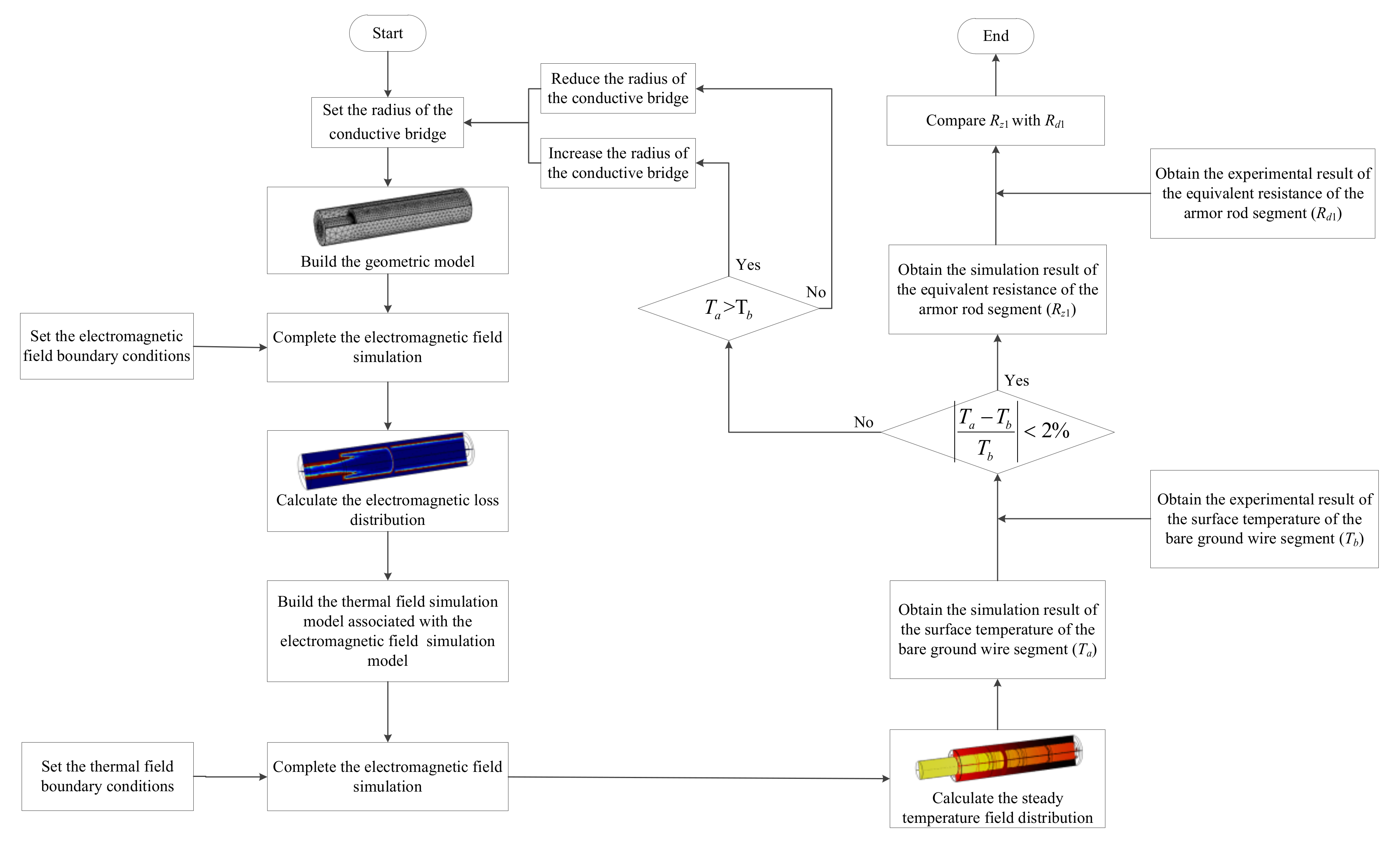
4.3. Determination of the Conductive Bridge Radius r

Based on the analysis in Section 2.2, for the 3D-EM model of the contact terminal, different contact cases between the ground wire and the armor rod can be simulated by changing the conductive bridge radius r. Therefore, determining the value of r in the 3D-EM model of the contact terminal is the premise of using the model for computing Rz1. In this paper, based on the coupling of the thermal field and the electromagnetic field, a method for determining the value of r in the 3D-EM model of the contact terminal was proposed. First, the three-dimensional thermal simulation model associated with the 3D-EM model of the contact terminal was established. Then, the value of r was determined by comparing the computational results of the thermal simulation model and the measurement results of the steady-state temperature rise experiments.
For the three-dimensional thermal simulation model of the contact terminal, part of the geometric parameters are shown in Table 1, and the axial lengths of the armor rod segment and the bare ground wire segment were both set to 100 mm. Then, the established three-dimensional thermal simulation model of the contact terminal is shown in Figure 14a. Combined with the analysis of Figure 12 in Section 4.1, it was inferred that in the case of a load less than 76 A, the radial sections of the ground wire and the armor rod at an axial distance of 100 mm from the contact surface could be considered as the axial adiabatic plane in the three-dimensional thermal simulation model of the contact terminal.
As the surfaces of the bare ground wire segment and the armor rod segment came into contact with air, the third type of thermal boundary condition was applied to the surfaces. The controlling equation of the third type of thermal boundary condition is shown in Equation (9). In Equation (9), TW is the surface temperature of the contact terminal; Tf is the temperature of the surrounding air; h is the natural heat transfer coefficient; n is the outer normal of the heat exchange surface; and W represents the external surface of the contact terminal:
λ ( T n ) W = h ( T W T f )
To visualize the specific settings of the thermal boundary conditions in the thermal simulation model of the contact terminal, the two-dimensional axial section of the contact terminal (Figure 14b) was presented for further explanation:
  • For Boundary I1 and I3, which belong to the horizontal boundaries, their natural heat transfer coefficients, h1 and h3, respectively, were automatically computed by COMSOL after inputting the ambient temperature and the diameters of the ground wire and the armor rod to COMSOL.
  • For Boundary I2, which belongs to the vertical boundaries, the natural heat transfer coefficient h2 was automatically computed by COMSOL after inputting the ambient temperature and the vertical height of Boundary I2 to COMSOL.
  • Boundary I4 was set as the axial adiabatic plane, i.e., the second type of thermal boundary condition.
The electromagnetic loss power of various components computed by the 3D-EM model of the contact terminal was adopted as the heat sources of corresponding components in the thermal simulation model of the contact terminal after processing, which was achieved by MATLAB. When using the above method to load heat source in the thermal simulation model of the contact terminal, it was necessary to note that the electromagnetic loss power output by the 3D-EM model was computed at 20 °C. Therefore, the relationship between the electromagnetic loss power and temperature should be taken into consideration. A conversion relationship between the electromagnetic loss power computed by the 3D-EM model of the contact terminal and the heat source loading in the thermal simulation model of the contact terminal existed, as shown in Equation (10):
P T = i 2 r 20 [ 1 + α ( T 20 ) ] = P 20 [ 1 + α ( T 20 ) ]
In Equation (10), PT is the heat source power at the temperature T; i is the loading current; r20 is the resistance at 20 °C; α is the temperature coefficient of steel; T is the conductor temperature; and P20 is the heat source power at 20 °C, i.e., the electromagnetic loss power output by the 3D-EM model.
In summary, the correlations between the electromagnetic field simulation model and the thermal field simulation model of the contact terminal can be mainly reflected in three points, as shown in Figure 15:
1)
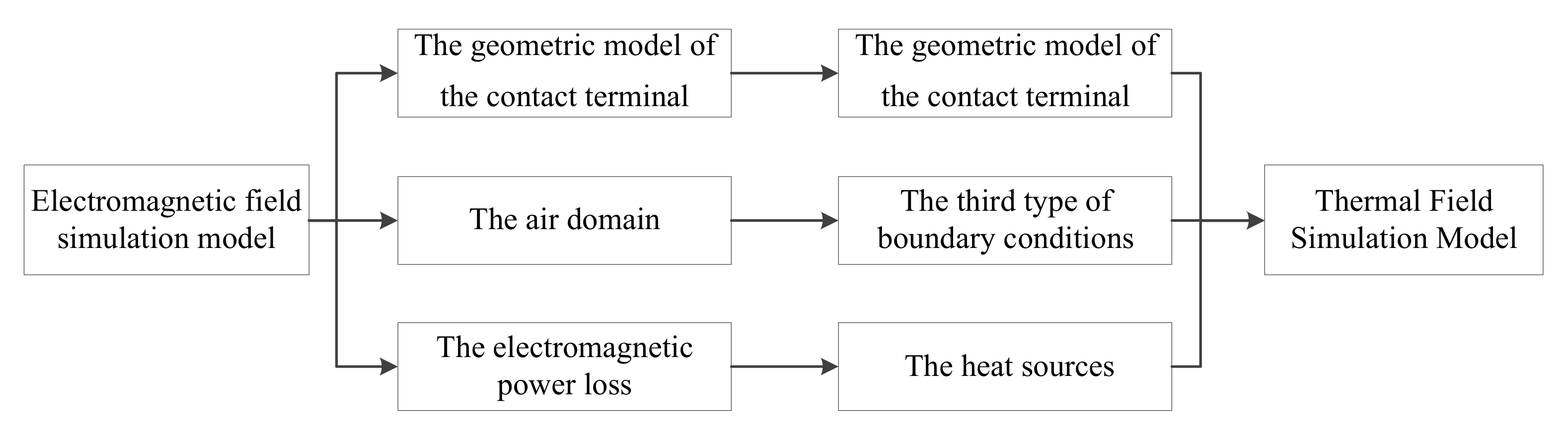
The geometric models of the contact terminal in the electromagnetic field simulation model and the thermal field simulation model were the same.
2)
In the thermal field simulation model, the third type of thermal boundary condition was used to simulate the air domain wrapped around the ground wire and the armor rod in the 3D-EM model.
3)
There was a conversion relationship between the electromagnetic loss power of various components computed by the 3D-EM model and the heat source of corresponding components in the thermal simulation model.
Combined with Figure 15, this indicated that the variation of the conductive bridge radius r led to the variation of the electromagnetic loss power output by the 3D-EM model of the contact terminal, which further led to the variation of the temperature distribution computed by the thermal simulation model of the contact terminal. Thus, the conductive bridge radius r and the temperature distribution of the contact terminal were correlated by the electromagnetic simulation model and the thermal simulation model. Based on the two simulation models of contact terminal, the surface temperature at the eleven temperature measuring points in Figure 11b could be computed under the premise that the conductive bridge radius was r. To evaluate the degree of fit between the surface temperature distribution curve calculated by simulation models and measured surface temperature distribution curve, the sum of square for the simulation result error at various temperature measuring points (i.e., Ssqu) was chosen as the index, which can be calculated by Equation (11). Obviously, the value of Ssqu was associated with r. The minimum value of Ssqu could be found by adjusting the value of r, and for the case of minimum Ssqu occurring, the simulation curve and the measured curve fit well. Thus, r corresponding to minimum Ssqu was regarded as the conductive bridge radius that enabled the temperature distribution in the thermal simulation model of the contact terminal to coincide with the actual distribution:
S s q u = i = 1 11 ( T a i T b i T a i ) 2
where Tai is the simulated surface temperature at temperature measuring point i, and Tbi is the measured surface temperature at temperature measuring point i. For the simulation model in this paper, if the variation of r was less than 0.0005 mm, the changes in temperature field of contact terminal could be negligible. Therefore, the minimum variation of r was set to 0.0005 mm when adjusting the value of r in this paper. Then, the conductive bridge radii under different loads were calculated, as shown in Table 3.
It was inferred from Table 3 that under the condition that the steady-state temperature change of contact terminal was not significant, the conductive bridge radius r hardly varied with the load. This phenomenon can be explained by the following. The deformation of contact terminal arising from the inapparent temperature change of the contact terminal could be ignored. Thus, the load variation had little influence on the contact condition between the ground wire and armor rod, which was reflected by the conductive bridge radius r. In the remaining part of Section 4, the conductive bridge radius r was set to 0.0340 mm for the experimental contact terminal.
To verify whether the conductive bridge radius r determined by the above method could make the temperature distribution in the thermal simulation model of contact terminal coincide with the actual distribution, the simulation results and experimental results of the steady state temperature of contact terminal under different loads were compared in Figure 16a. With reference to the experimental results, an error analysis of the thermal simulation model was conducted in Figure 16b. Based on Figure 16a,b, it was concluded that the axial surface temperature distribution curves of the contact terminal calculated by the thermal simulation model basically matched the actual measured axial surface temperature distribution curves. Moreover, the absolute error in the thermal simulation model of the steady state surface temperature was less than 9%. Thus, the conductive bridge radii determined by Equation (11) had sufficient accuracy to be applied in the 3D-EM model and the thermal simulation model of contact terminal.

4.4. Discussion

Based on the conductive bridge radius r determined in Section 4.3 for the experimental contact terminal, Rz1 output by the 3D-EM model of the experimental contact terminal was computed. With reference to the measured result Rd1 in Section 4.2, an error analysis of the 3D-EM model of the contact terminal was conducted in Table 4.
1)
The value of the Rz1 output by the 3D-EM model of contact terminal was dependent on the value of the conductive bridge radius r, and the value of conductive bridge radius r was dependent on the error between the calculation results of thermal simulation model and the measuring results of the steady-state temperature rise experiments. Therefore, the calculation error of the conductive bridge radius r accumulated in the calculation error of Rz1 inevitably.
2)
Table 4 shows that for the experimental contact terminal, the calculation error of Rz1 in the 3D-EM model was 3.0%. Thus, the 3D-EM model of contact terminal was sufficiently accurate to be practically applied to calculate the value of Rz1.
In conclusion, the reliability of the 3D-EM model of the contact terminal proposed in this paper was verified. The whole experimental verification process is shown in Figure 17. Thus, the 3D-EM model of the contact terminal could provide reliable data for the analysis of influencing factors on Rz1 discussed in the next section.

5. Analysis of Factors Influencing Rz1

Given that the duration of current flowing through the ground wire is short, heat exchange between the ground wire and environment can be negligible and the temperature rise of ground wire is mainly dependent on its heat production. Therefore, Rz1 can be regarded as an indicator to evaluate the temperature rise of the armor rod segment in the contact terminal. The analysis in Section 3 pointed out that the calculation result of the contact terminal’s 3D-EM model mainly depended on the action of the skin effect and the distribution characteristics of the contact points. Thus, the effects of the three factors (μr, θ, and l) on Rz1 are subsequently discussed.
To investigate the effect of μr on Rz1, the values of Rz1 under different relative permeability were calculated with an r of 0.06 mm, l of 4.12 mm, θ of 22°, and load current of 100 A in the 3D-EM model of the contact terminal, as shown in Figure 18. Meanwhile, the change of L with μr is also presented in Figure 18.
It can be seen from Figure 18 that the calculation results of Rz1 and L tend to linearly increase with the increasing μr. With the increase of μr, the degree of the skin effect intensifies, which results in more uneven current distribution in contact terminal. In general, the more uneven the current density distribution in a conductive path is, the larger the corresponding equivalent resistance is. As a result, the trend of curves in Figure 18 is explained.
Calculation results of Rz1 and L under different θ are shown in Figure 19 with r of 0.06 mm, μr of 1000, l of 3.7 mm and load current of 100 A. Figure 19 shows that the value of Rz1 and L hardly varies with θ. This phenomenon is mainly caused by the radial symmetric distribution of the current density and the contact points in the contact terminal. The variation of θ only means that the transverse sections including the contact points rotates along the tangent of the radial, but it has no influence on the axial distance between two transverse sections. Thus, the variation of θ doesn’t affect the current diffusion near the contact surface.
Calculation results of Rz1 and L under different l are shown in Figure 20 with an r of 0.06 mm, μr of 1000, θ of 22 and load current of 100 A. Figure 20 shows that the value of Rz1 and L increased with the increasing l. With the increase of l, the number of conductive bridges within the same current diffusion range decreased, which led to the reduction in contact area between the ground wire and armor rod. As a result, the corresponding contact resistance increased with the increase of l. To further explain the relationship between Rz1 and l, the axial sampling results of current density (the sampling path in Figure 10b) under different l are shown in Figure 21.
In Figure 21a, the axial positions of the first peak of the sampling result curves under different l almost coincide. However, the axial positions of the second peak are associated with l, and the smaller the value of l, the closer the axial position of the second peak is to the contact surface. In Figure 21b, it can be inferred that the current flowing through the first row of conductive bridges increased with the increase of l. This intensified the unevenness of the current distribution in the current diffusion range, which resulted in the increase of Rz1.
Based on the above analysis, Rz1 is only influenced by l for the two parameters (l and θ) describing the distribution characteristics of the contact points between the ground wire and armor rod. Thus, the effects of the stranding directions and lay lengths of ground wire and armor rod on Rz1 can be investigated by l.
In conclusion, for the case of contact terminal with larger μr or l, the value of Rz1 was larger, which means that the temperature rise was higher. As a result, the breakage possibility of the armor rod segment in contact terminal may increase.

6. Conclusions

The main conclusions of this work may be summarized as follows:
1)
This paper adopted the cylindrical conductive bridge model to simulate the conductive contact points between the ground wire and armor rod, and subsequently established a 3D-EM model of the contact terminal based on the actual characteristics of contact points. The 3D-EM model was successfully applied to obtain the current distribution in the contact terminal.
2)
The simulation results of the 3D-EM model showed that the current diffusion occurred near the contact surface and the severe current contraction phenomenon happened in the conductive bridges within the diffusion range. However, outside the current diffusion range, there was no current exchange between the ground wire and armor rod. As a result, the contact resistance generating heat effect near the contact surface was only determined by the conductive bridges within the current diffusion range.
3)
This paper proposed a method for determining the conductive bridge radius r, which was based on the criterion of the minimum sum of squared error between the simulation results and experimental results at the temperature measurement points of contact terminal. The results of the steady state temperature rise experiments for contact terminal verified that the conductive bridge radius r determined by the proposed method could have sufficient accuracy for application in the 3D-EM model and the thermal simulation model of contact terminal.
4)
Rz1 could be regarded as an indicator to evaluate the temperature rise of the armor rod segment in the contact terminal. The results of the equivalent resistance measuring experiments for the armor rod segment verified that the 3D-EM model of contact terminal developed in this paper was sufficiently accurate to be practically applied to calculate the value of Rz1 .This meant that the 3D-EM model could provide reliable data for analyzing breakage accidents of the armor rod segment in contact terminal caused by temperature rise.
5)
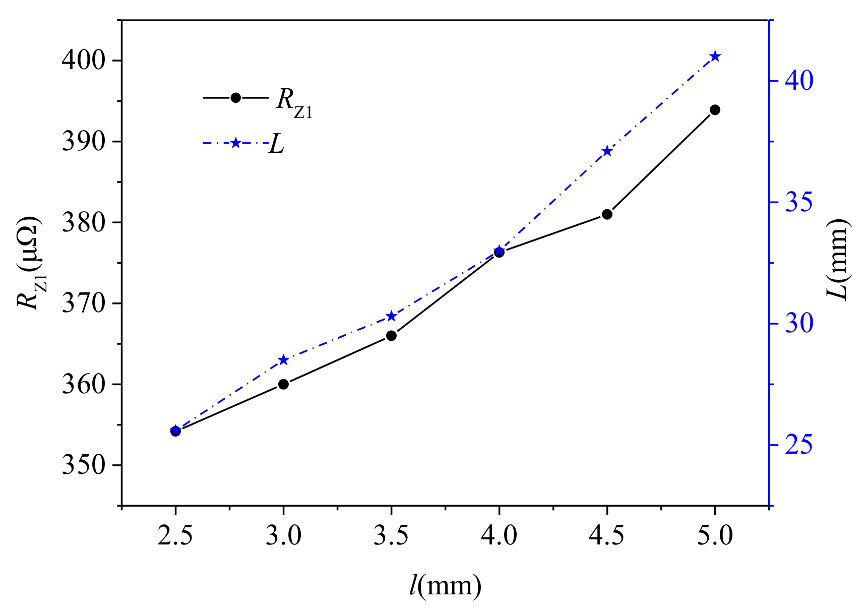
Based on the 3D-EM model of contact terminal, the values of Rz1 under different μr, θ, and l were calculated, respectively. The results showed that the value of Rz1 hardly varied with θ. However, the increasing l and μr resulted in a larger Rz1, which could increase the breakage possibility of the armor rod segment in contact terminal.

Acknowledgments

The authors gratefully acknowledge the Dongguan Power Supply Bureau of the Guangdong Power Grid Co., Ltd. The authors would also like to thank the anonymous reviewers for their instructive comments.

Author Contributions

This paper is a result of the collaboration between all co-authors. Gang Liu conceived and designed the study. Deming Guo established the simulation model. Pengyu Wang wrote the paper. Honglei Deng helped with the corrections. Xiaobin Hong designed and performed the temperature rise experiments. Wenhu Tang designed and performed the measurement experiments of the equivalent resistance for the armor rod segment.

Conflicts of Interest

The authors declare no conflict of interest.

Nomenclature

Variables
lAxial distance between adjacent two radial cross section of the armor rod segment with contact points (mm).
l1Axial distance between adjacent two radial cross section of the armor rod segment with contact points when the stranding directions of the outermost layer of the ground wire and the armor rod are identical (mm).
l2Axial distance between adjacent two radial cross section of the armor rod segment with contact points when the stranding directions of the outermost layer of the ground wire and the armor rod are opposite (mm).
s1Lay length of the outermost layer of the ground wire (mm).
s2Lay length of the outermost layer of the armor rod (mm).
θRotation angle of the adjacent two contact points on the stranded conductor of the outermost layer of the same strand of ground wire.
θ1Rotation angle of the two adjacent contact points on the stranded conductor of the outermost layer of the same strand of ground when the stranding directions of the outermost layer of the ground wire and the armor rod are identical.
θ2Rotation angle of the two adjacent contact points on the stranded conductor of the outermost layer of the same strand of ground when the stranding directions of the outermost layer of the ground wire and the armor rod are opposite.
sminMinimum value between s1 and s2 (mm).
HHeight of cylindrical conductive bridge model (mm).
rRadius of cylindrical conductive bridge model (mm).
R1DC resistance of the ground wire (Ω).
R2Power frequency AC resistance of the ground wire (Ω).
S1Equivalent sectional areas of the ground wire through which direct current pass (m2).
S2Equivalent sectional areas of the ground wire through which power frequency alternating current pass (m2).
rgRadius of the ground wire (m).
dSkin depth of steel under the power frequency of 50 Hz (m).
ωAngular frequency (rad/s).
μrRelative permeability of steel.
μ0Vacuum magnetic conductivity (N/A2).
γConductivity of steel (S/m).
LAxial length of the current diffusion range of the armor rod segment (mm).
Rz1Equivalent resistance of the armor rod segment (Ω).
RzTotal resistance of the simulation model (Ω).
R20Resistance of the bare ground wire segment in the simulation model (Ω).
UOutput voltage of the adjustable constant alternating current source (V).
cosφPower factor of measuring loop.
IOutput current of the adjustable constant alternating current source (A).
RTotal resistance of the constant-current source lead, parallel groove clamp, and the measurement segment of the experimental ground wire (Ω).
Rd1Resistance of the measurement segment of the experimental ground wire (Ω).
Rf1Total AC resistance of the constant-current source lead L1 and the corresponding parallel groove clamp (Ω).
Rf2Total AC resistance of the constant-current source lead L2 and the corresponding parallel groove clamp (Ω).
Rf1′Total measured DC resistance of the constant-current source lead L1 and the corresponding parallel groove clamp (Ω).
Rf2′Total measured DC resistance of the constant-current source lead L2 and the corresponding parallel groove clamp (Ω).
TWSurface temperature of the contact terminal (°C).
TfTemperature of the surrounding air (°C).
hNatural heat transfer coefficient (W/(m2·K)).
PTHeat source power at the temperature T (W).
TConductor temperature (°C).
iLoad current (A).
r20Resistance at 20 °C (Ω).
αTemperature coefficient of steel (°C−1).
P20Heat source power at 20 °C, i.e., the electromagnetic loss power output by the 3D-EM model (W).
SsquSum of square for the simulation result error at various temperature measuring points.
TaiSimulated surface temperature at temperature measuring point i (°C).
TbiMeasured surface temperature at temperature measuring point i (°C).
Parameters and Constants
FEAFinite element analysis.
3D-EM modelThree-dimensional electromagnetic field simulation model based on the multiple contact points model.
A1Terminal of the bare ground wire segment.
A2Terminal of the armor rod segment.
ACurrent density sampling path at the radial terminal of the armor rod segment away from the contact surface.
BCurrent density sampling path at the radial terminal of the bare ground wire segment away from the contact surface.
L1A constant-current source Lead.
L2The other constant-current source Lead.
nOuter normal of the heat exchange surface.
WExternal surface of the contact terminal.
I1Horizontal surface boundary of the bare ground wire segment in the thermal model.
I2Vertical surface boundary of the armor rod segment at the contact surface in the thermal model.
I3Horizontal surface boundary of the armor rod segment in the thermal model.
I4Both of the two radial cross sections at the ends of the thermal model.

References

  1. Jiang, X.; Meng, Z.; Zhang, Z.; Hu, J.; Lei, Y. DC ice-melting and temperature variation of optical fiber for ice-covered overhead ground wire. IET Gener. Transm. Distrib. 2016, 10, 352–358. [Google Scholar] [CrossRef]
  2. Li, J.; Sun, D. Analysis on Lightning Strike Damages to Optical Fiber Composite Overhead Ground Wire. In Proceedings of the 2009 International Conference on Industrial and Information Systems, Haikou, China, 24–25 April 2009; pp. 39–44. [Google Scholar]
  3. Du, T.; Zhang, Y.; Xia, W. Study on the Problem of Lightning Strike OPGW. In Proceedings of the 2006 International Conference on Power System Technology, Chongqing, China, 22–26 October 2006; pp. 1–4. [Google Scholar]
  4. Karabay, S.; Guven, E.A.; Erturk, A.T. Enhancement on Al–Mg–Si alloys against failure due to lightning arc occurred in energy transmission lines. Eng. Fail. Anal. 2013, 31, 153–160. [Google Scholar] [CrossRef]
  5. Karabay, S. Modification of Conductive Material AA6101 of OPGW Conductors against Lightning Strikes. Strojniski Vestnik J. Mech. Eng. 2013, 59, 451–461. [Google Scholar] [CrossRef]
  6. Iwata, M.; Ohtaka, T.; Goda, Y. Melting and Breaking of 80 mm2 OPGWs by DC Arc Discharge Simulating Lightning Strike. In Proceedings of the 2016 33rd International Conference on Lightning Protection (ICLP), Estoril, Portugal, 25–30 September 2016; pp. 1–4. [Google Scholar]
  7. Liu, G.; Li, Y.; Guo, D.; Qi, H.; Zhang, Y.; Ma, H. Experimental Investigation on the Breakage in Earth Wire Suspension String with Winding Preformed Armor Rods. In Proceedings of the 2017 IEEE International Conference on Environment and Electrical Engineering and 2017 IEEE Industrial and Commercial Power Systems Europe (EEEIC/I&CPS Europe), Milan, Italy, 6–9 June 2017; pp. 1–5. [Google Scholar]
  8. Andrusca, M.; Adam, M.; Burlica, R.; Munteanu, A.; Dragomir, A. Considerations regarding the Influence of Contact Resistance on the Contacts of Low Voltage Electrical Equipment. In Proceedings of the 9th International Conference and Exposition on Electrical and Power Engineering (EPE), Iasi, Romania, 20–22 October 2016; pp. 123–128. [Google Scholar]
  9. Holm, R. Electrical Contacts, 4th ed.; Springer: New York, NY, USA, 1979. [Google Scholar]
  10. Greenwood, J.A. Constriction Resistance and the Real Area of Contact. Br. J. Appl. Phys. 1966, 17, 1621–1632. [Google Scholar] [CrossRef]
  11. Kogut, L.; Komvopoulos, K. Electrical contact resistance theory for conductive rough surfaces. J. Appl. Phys. 2003, 94, 3153–3162. [Google Scholar] [CrossRef]
  12. Laor, A.; Herrell, P.J.; Mayer, M. A Study on Measuring Contact Resistance of Ball Bonds on Thin Metallization. IEEE Trans. Compon. Packag. Manuf. Technol. 2015, 5, 704–708. [Google Scholar] [CrossRef]
  13. Dhotre, M.T.; Korbel, J.; Ye, X.; Ostrowski, J.; Kotilainen, S.; Kriegel, M. CFD Simulation of Temperature Rise in High-Voltage Circuit Breakers. IEEE Trans. Power Deliv. 2017, 32, 2530–2536. [Google Scholar] [CrossRef]
  14. Zeng, R.; Zhou, P.; Wang, S.; Li, Z.; Zhang, B. Modeling of Contact Resistance in Ground System and Analysis on Its Influencing Factors. High Volt. Eng. 2010, 36, 2393–2397. [Google Scholar] [CrossRef]
  15. Ito, S.; Kawase, Y.; Mori, H. 3-D finite element analysis of repulsion forces on contact systems in low voltage circuit breakers. IEEE Trans. Magn. 1996, 32, 1677–1680. [Google Scholar] [CrossRef]
  16. Qiang, R.; Rong, M. Simulation of the contact resistance of high voltage apparatus with the method of coupling contact surface. In Proceedings of the 2013 2nd International Conference on Electric Power Equipment—Switching Technology (ICEPE-ST), Matsue, Japan, 20–23 October 2013; pp. 1–4. [Google Scholar]
  17. Li, X.; Qu, J.; Wang, Q.; Zhao, H.; Chen, D. Numerical and Experimental Study of the Short-Time Withstand Current Capability for Air Circuit Breaker. Trans. Power Deliv. 2013, 28, 2610–2615. [Google Scholar] [CrossRef]
  18. Li, X.; Chen, D. 3-D Finite Element Analysis and Experimental Investigation of Electrodynamic Repulsion Force in Molded Case Circuit Breakers. IEEE Trans. Compon. Packag. Manuf. Technol. 2005, 28, 877–883. [Google Scholar] [CrossRef]
  19. Kawase, Y.; Mori, H.; Ito, S. 3-D finite element analysis of electrodynamic repulsion forces in stationary electric contacts taking into account asymmetric shape (invited). IEEE Trans. Magn. 1997, 33, 1994–1999. [Google Scholar] [CrossRef]
  20. Kong, W.; Cheng, Y. Measures of Introduction and Look Forward to Prevent Breeze Vibration of Overhead Power Transmission Lines. In Proceedings of the 2011 Second International Conference on Mechanic Automation and Control Engineering, Hohhot, China, 15–17 July 2011; pp. 2299–2301. [Google Scholar]
  21. Dai, D.; Zhang, X.; Wang, J. Calculation of AC Resistance for Stranded Single-Core Power Cable Conductors. IEEE Trans. Magn. 2014, 50, 1–4. [Google Scholar] [CrossRef]
  22. De Paulis, F.; Olivieri, C.; Orlandi, A.; Giannuzzi, G.; Bassi, F.; Morandini, C.; Fiorucci, E.; Bucci, G. Exploring Remote Monitoring of Degraded Compression and Bolted Joints in HV Power Transmission Lines. IEEE Trans. Power Deliv. 2016, 31, 2179–2187. [Google Scholar] [CrossRef]
  23. Hao, X.; Yin, W.; Strangwood, M.; Peyton, A.; Morris, P.; Davis, C. Characterization of Decarburization of Steels Using a Multifrequency Electromagnetic Sensor: Experiment and Modeling. Metall. Mater. Trans. A 2009, 40, 745–756. [Google Scholar] [CrossRef]
  24. Guo, D.; Liu, G.; Qi, H.; Zhang, Y. Experimental analysis on temperature distribution of ground wire suspension string with winding preformed armor rod. Guangdong Electr. Power 2017, 30, 1–5. [Google Scholar] [CrossRef]
  25. Wang, P.; Liu, G.; Ma, H.; Liu, Y.; Xu, T. Investigation of the Ampacity of a Prefabricated Straight-Through Joint of High Voltage Cable. Energies 2017, 10, 2050. [Google Scholar] [CrossRef]
  26. Liu, G.; Lei, M.; Ruan, B.; Zhou, F.; Li, Y.; Liu, Y. Model research of real-time calculation for single-core cable temperature considering axial heat transfer. High Volt. Eng. 2012, 38, 1877–1883. [Google Scholar] [CrossRef]
  27. You, L.; Wang, J.; Liu, G.; Ma, H.; Zheng, M. Thermal rating of offshore wind farm cables installed in ventilated J-tubes. Energies 2018, 11, 545. [Google Scholar] [CrossRef]
Figure 1. Schematic of the contact terminal consisted of ground wire and armor rod.
Energies 11 00737 g001
Figure 2. Radial section of the armor rod segment. (a) case 1 with contact points; (b) the transitional stage without contact points; (c) case 2 with contact points.
Energies 11 00737 g002
Figure 3. Spatial distribution of the contact points between ground wire and armor rod.
Energies 11 00737 g003
Figure 4. Radial section with contact points of the armor rod segment in the multiple contact points simulation model.
Energies 11 00737 g004
Figure 5. 3D geometric model of the contact terminal.
Energies 11 00737 g005
Figure 6. Electromagnetic field boundary conditions of the 3D-EM model of the contact terminal.
Energies 11 00737 g006
Figure 7. Determination of the axial length of the 3D-EM model.
Energies 11 00737 g007
Figure 8. Current density distribution of the contact terminal: (a) 3D current density distribution of the contact terminal; (b) 2D axial section of the current density distribution near the contact surface; and (c) 2D magnification diagram of the current density distribution near the first row of conductive bridges in Figure 8b.
Energies 11 00737 g008
Figure 9. Radial sampling results of current density distribution in the 3D-EM model: (a) sampling path; and (b) sampling results.
Energies 11 00737 g009
Figure 10. Axial sampling results of current density distribution in the 3D-EM model: (a) sampling path; and (b) sampling results.
Energies 11 00737 g010
Figure 11. System of the temperature rise experiments: (a) schematic of the experimental setup; and (b) schematic of the temperature measurement system.
Energies 11 00737 g011
Figure 12. Steady-state axial temperature distribution of the contact terminal under different loads.
Energies 11 00737 g012
Figure 13. System of the equivalent resistance measurement experiment for the armor rod segment: (a) actual wiring diagram of the alternating current voltage drop method; (b) actual wiring diagram of the digital DC bridge measuring method; and (c) schematic of the experimental setup.
Energies 11 00737 g013
Figure 14. 3D thermal simulation model of the contact terminal: (a) 3D geometric model; and (b) 2D axial section of the contact terminal.
Energies 11 00737 g014
Figure 15. Correlations between the electromagnetic field simulation model and the thermal field simulation model of the contact terminal.
Energies 11 00737 g015
Figure 16. Comparisons between experimental and simulation results under different currents: (a) comparison of the steady state temperature distribution in the contact terminal; and (b) modeling error analysis.
Energies 11 00737 g016
Figure 17. Flow diagram of the experimental verification process.
Energies 11 00737 g017
Figure 18. Result curves of Rz1 and L under different μr.
Energies 11 00737 g018
Figure 19. Result curves of Rz1 and L under different θ.
Energies 11 00737 g019
Figure 20. Result curves of Rz1 and L under different l.
Energies 11 00737 g020
Figure 21. Axial sampling results of current density distribution (the sampling path in Figure 10b) under different l: (a) sampling results of the whole contact terminal; and (b) magnification diagram near the first peak in Figure 21a.
Energies 11 00737 g021
Table 1. Relevant geometric parameters of the 3D-EM model of the contact terminal.
Model ComponentsGeometric Parameters (mm)
Radius of the ground wire4.5
Thickness of the armor rod3.6
Height of the conductive bridge/air gap0.1
Radius of the air field10
Table 2. Physical parameters of the steel.
Physical PropertiesValue
Conductivity (S/m)6 × 106
Relative permeability300~4000
Relative permittivity1
Thermal conductivity (W/(m·K))420
Table 3. Calculation results of the conductive bridge radii under different currents.
Current (A)SsquConductive Bridge Radii (mm)
550.03070.0340
680.03580.0335
760.03670.0340
Table 4. Comparisons between experimental and calculated results of the equivalent resistance.
Conductive Bridge Radius r (mm)Rd1 (μΩ)Rz1 (μΩ)Relative Error
0.0340655.9675.33.0%

