Abstract
To improve our capacity to use available wind speed data, it is necessary to develop a new statistical temporal downscaling method that uses one or a few input variables of any temporal scale for mean wind speed data to obtain wind statistics at finer temporal resolution. In the present study, a novel statistical temporal downscaling method for wind speed statistics and probability distribution is proposed. The proposed method uses the temporal structure to downscale the wind speed statistics to a fine temporal scale without the use of additional variables. The Weibull distribution of the hourly and 10-min mean wind speed data is obtained by the downscaled wind speed statistics. The proposed method provides the downscaled Weibull distribution of fine temporal wind speed data using coarse temporal wind statistics. Particularly, the use of sub-daily mean wind speed data in the downscaling of the wind speed Weibull distribution leads to good estimation precision. The Weibull distribution downscaled by the proposed method successfully reproduces the wind power density based on the wind potential energy estimation.
1. Introduction
When planning wind farms, many regions that are expected to have a large wind power potential do not have weather stations that can measure wind speed. For example, many offshore regions do not have weather stations or wind speed measuring instruments. To assess the wind power potential in a region that does not have wind speed observations, the development of advanced climate models and remote sensing techniques allow for the use of various wind speed observations or estimates for investigations of the characteristics of wind speed data and wind power potential assessments in many regions [1,2,3]. Gadad and Deka [4] assessed the wind power potential of offshore regions along the west coast of India using Oceansat-2 scatterometer (OSCAT) wind speed data. The OSCAT wind speed data can be used for wind power potential assessments in this region, where there is a scarcity of in situ wind speed data. These data improve our capacity to model wind speed and assess the wind power potential in these regions. However, the temporal and spatial scales of these wind observations and estimates are relatively coarse for investigating the detailed characteristics of the wind potential energy. Wind speed observations and estimates at a finer scale are required for an accurate wind power potential assessment.
To obtain fine-scale meteorological data from coarse-scale data, downscaling methods have been widely employed [5,6,7,8,9]. Two categories are used in the downscaling methods: (1) dynamical downscaling and (2) statistical downscaling [10,11]. The dynamical downscaling method uses regional climate models (RCMs) to simulate various climatic variables at fine temporal and spatial scales. Because dynamical downscaling can respond in physically consistent ways to external conditions, the dynamical downscaling method is theoretically preferable. The statistical downscaling method, which is considered an empirical downscaling method, uses empirical relationships between a variable of interest and predictors to obtain the variable at fine temporal or spatial scales. In certain cases, the statistical downscaling method can reproduce the statistical characteristics of variables improperly simulated by the dynamical downscaling methods. The statistical downscaling method also needs a smaller number of predictors than the dynamical downscaling method and is computationally more efficient.
Both downscaling methods have been widely applied in many studies focused on downscaling wind speed data to fine spatial or temporal resolution [12,13,14,15,16,17,18,19,20,21]. As mentioned above, wind speed data at a fine spatial resolution are required to design the wind farm. Many spatial wind observations or estimates have a coarse spatial resolution. Additionally, certain wind speed simulations from dynamical models improperly reproduce wind speed statistics. To resolve these drawbacks, many spatial downscaling methods have been developed and studied.
Pryor et al. [22] employed a dynamical downscaling method to examine the impact of climate change on the near-surface flow and wind energy density across northern Europe. In their study, a RCM was employed to downscale wind speed as well as other meteorological variables. This study showed that the simulated wind fields present reasonable and realistic results. Pryor et al. [23] proposed an empirical spatial downscaling method for wind speed probability distributions and used parameters of the Weibull distribution as predictands of the downscaling method. Predicting the Weibull parameters led to a more accurate wind power estimate compared with the results of the dynamical downscaling method, which produces wind speed series. Horvath et al. [20] applied the dynamical downscaling method for wind speed in complex terrain, and they compared the performance of three dynamical downscaling methods for wind speed downscaling based on the spatial distribution, wind statistics and spectral analysis. These authors found that the dynamical adaptation method provides the best performance among the investigated methods. Devis et al. [24] proposed a new statistical method for downscaling wind speed probability distributions. In their study, the parameters of the wind speed probability distributions for mean wind speed data and climatic variables were used as the predictands and predictors of the downscaling method, respectively.
Although a number of studies have focused on developing statistical and dynamical spatial downscaling methods for variables related to wind speed characteristics, a limited number of studies have attempted to develop a statistical temporal downscaling method for the variables related to wind speed characteristics. Kumar et al. [25] used a neural network with global climate model outputs and meteorological observations to obtain the downscaled meteorological variables. In their study, they used monthly data to calculate 6-hour meteorological variables, and their method successfully reproduced a number of meteorological variables. The temporal downscaling method proposed by Kumar et al. [25] requires a considerable number of input variables, such as climatic variables, from climate models for the downscaling method. However, such a large number of climatic data are often unavailable in many regions.
Guo et al. [26] proposed a temporal downscaling method using the diurnal pattern of hourly wind speed data. In their method, daily mean wind speed data were downscaled to hourly wind speed data. The method proposed by Guo et al. [26] used daily mean wind speed data or daily mean and max wind speed data in the downscaling method. Because the diurnal pattern of wind speed data was used to downscale, the wind speed data of different temporal scales, e.g., 7-h, 2-day and 3-day, cannot be used in this method.
The temporal downscaling methods proposed in the previous studies have certain limitations for application in the wind power potential assessment. To use a downscaling method for wind power potential assessment, the method can only use wind speed data that successfully reproduces the statistics of wind speed data at a fine resolution. When few data are available, such as for in situ observations and other meteorological variables, the temporal downscaling method often needs to be employed. Additionally, estimating precise wind statistics at a fine temporal scale is important in the wind power potential assessment because the statistics represent the probability distribution of the data. Thus, a new temporal downscaling method that simultaneously satisfies two conditions must be developed for temporally downscaling wind speed data in wind power potential assessments.
The aim of the present study is to propose a novel temporal downscaling method for wind speed statistics and probability distributions. Because the method proposed in the current study uses the temporal structure to downscale the wind speed statistics to a fine temporal scale, wind statistics can be downscaled by the proposed method without any other information and variables. Furthermore, because the proposed method uses wind statistics instead of wind speed data, the downscaled wind statistics from the proposed method may preserve the original wind statistics well. The wind speed probability distribution at the fine temporal scale can be obtained by the downscaled wind speed statistics. To the best of our knowledge, the scaling property has not been employed in downscaling wind speed distribution yet. This method is also simple and computationally efficient. The results of current study contribute to improve our understanding of wind power potential assessments in regions where wind speed data at a fine temporal resolution are scarce. Additionally, the proposed method promotes the use of wind speed data at a coarse temporal scale for wind power potential assessment of these regions.
This paper is organized as follows: in Section 2, the proposed temporal downscaling method is described. In Section 3, detailed information is provided on the methodology for the temporal downscaling method proposed in the current study. In Section 4, the data description and cases used in the applications are presented. In Section 5, the evaluation criteria results are provided and the applicability and performance of the proposed method for Weibull parameter and wind potential energy estimations are discussed. Finally, in Section 6, the conclusions are presented.
2. A Novel Method to Downscale Wind Speed Probability Distribution
To investigate the statistical characteristics of various hydro-meteorological variables, their scaling properties have been examined [27,28,29,30,31,32,33,34,35,36,37]. In wind speed analyses, the scaling (fractal) property has been employed to investigate the temporal structure of wind speed data [38,39,40,41,42,43]. In these studies, the relationship between the fluctuation function of wind speed data and their temporal scales have been employed to examine the temporal structure of the wind speed data. The current study uses a different and simple method of investigating the statistical behavior of the mean wind speed data versus temporal scales. Additionally, a temporal downscaling method is developed based on the temporal structure of the statistical characteristics for mean wind speed data.
In the current study, we use the relationship between sample cumulative raw moments (CRMs) of wind speed and their temporal scales. The sample CRM is expressed by Equation (1):
where and n are the i-th wind speed data and the number of wind speed data, respectively. Figure 1 presents the CRM log of the wind speed data at 10 m height corresponding to the log of temporal scales at six stations in South Korea.
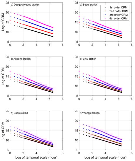
Figure 1.
Plot of the log of the CRMs of wind speed and log of the temporal scales for the 1st- to 4th-order CRMs of six stations: (a) Daegwallyeong, (b) Seoul, (c) Andong, (d) Jinju, (e) Buan, (f) Yeongju stations.
Strong linear relationships are observed between the log of the CRMs and the log of the temporal scales. The linear relationships can be used to obtain the linear models, which represent the temporal structure of wind speed statistics. The wind speed statistics at a fine temporal scale are obtained from the linear models. The procedure of the proposed temporal downscaling method is described as follows:
- (1)
- Calculate the CRMs (1st to 4th orders) of the wind speed data corresponding to coarse temporal scales. For example, when daily mean wind speed data are available, the mean wind speeds of coarser temporal scales, i.e., 2-day, 3-day, and 4-day, are calculated by aggregating the daily mean wind speed data. The CRMs of the daily, 2-, 3-, and 4-day mean wind speed data are calculated.
- (2)
- Build a linear model between the log of the CRMs and the log of the temporal scales.
- (3)
- Estimate the CRMs corresponding to the fine temporal scale of interest, e.g., 1-h from the linear model built in step (2). For simplicity, the target temporal scale of wind speed statistics is 1-h in this study.
- (4)
- Convert the CRM estimates in step (3) to central moments. Because the CRMs cannot be directly applied to fit the probability distribution, they must be converted to central moments that are usually used in the method of moments.
- (5)
- Estimate the parameters of the selected probability distribution by the method of moments with central moment estimates in step (4). The proposed method can be employed for any probability distribution that can be fitted by the method of moments. For simplicity, the current study focuses on the Weibull distribution.
- (6)
- Calculate the wind potential energy using the probability distribution with the parameter estimates in step (5).
3. Methods
3.1. Fitting Methods of a Linear Regression Model
In the current study, the ordinary least square (OLS) and weight least square (WLS) methods are employed for the fitting of a linear model for the relation between the log of the CRM and the log of the temporal scale of the mean wind speed data. The OLS method is frequently employed to fit a linear model. The linear model is written as follows:
where Y is the log of the CRM ( matrix), with m representing the number of temporal scales used; X is the log of the temporal scale ( matrix); and b is the regression coefficient ( matrix). To take into account the intercept, X has two columns: one is the log of the temporal scale and the other is one. For the given linear model, the OLS estimator is expressed as follows:
The moments at fine temporal scales are considered more similar to the moments of hourly mean wind speed data than to the moments of coarse temporal scales. In the OLS method, all the independent variables (X) have the same weight in fitting the linear model. To improve the performance of predicting the moment of hourly mean wind speed, the information on moments at fine temporal scales (e.g., 2-h or 3-h mean wind speed data) should be considered to fit the linear model better. To take into consideration the temporal scales of the wind speed data, the WLS method is used in the current study. In the WLS, because the weight matrix used to assign different weights to each independent variable is added to fit the linear model, the fitted linear model may lead to a better predictive performance of the moments of the hourly mean wind speed. The WLS estimator is expressed as follows:
where W is weight matrix ( diagonal matrix). Setting the weight in the weight matrix plays a key role in the WLS method. In the current study, the weight matrix is employed in Equation (5):
where is log of the j-th temporal scale. The weight matrix used in the current study assigns a larger weight to the CRM when the temporal scale of the CRM is finer.
3.2. Moment Conversion
Because the CRMs cannot be directly used to fit a Weibull distribution, they have to be converted to central moments, which are commonly used in the method of moments. For the Weibull distribution, the raw moments can be used to obtain the moment estimates. However, for convenience and consistency with other studies, the central moments are used in the current study [44,45,46]. Thus, the moment conversion way is presented in this section. First, the CRM should be converted to a raw moment. The sample raw moment is calculated via Equation (6):
When the CRM and the number of data corresponding to the temporal scale of interest have been determined, the raw moment () can be obtained by Equation (6). Second, the raw moment is converted to the central moment. The sample central moment is expressed as follows:
where is the mean of . The raw moments that have an order higher than one can be converted to the central moment by Equations (9)–(11):
3.3. Method of Moment for Weibull Distribution
The method of moments is a traditional method for fitting probability models and was broadly applied to fit the probability distribution models [44,45,46]. The idea of the method of moments is to find the parameters of the probability distribution model such that the sample and theoretical central moments from the fitted probability distribution are the same. The central moments required in the method of moments differ depending on the probability distribution model. In the current study, the Weibull distribution is considered as the probability distribution of the mean wind speed data. An extensive body of literature reported that the application of the Weibull distribution in modeling wind speed data well reproduces the wind speed regime [47,48,49,50,51,52,53,54,55]. The probability density function of the Weibull distribution is expressed as follows:
where v, c, and k are the mean wind speed, scale parameter, and shape parameter, respectively. The theoretical 1st- and 2nd-order central moments of the Weibull distribution are expressed as follows:
where is the gamma function. The method of moments for the Weibull distribution identify the parameters that produce 1st and 2nd theoretical moments equivalent to the 1st and 2nd sample moments. This problem in the method of moments is solved by a numerical optimization method.
3.4. Evaluation Criteria
In the current study, bias, absolute bias (ABias), relative bias (RBias), and absolute relative bias (ARBias), root mean square error (RMSE) are employed for evaluating the performance of the proposed method. The equations of the evaluation criteria are expressed in Equations (15)–(19):
where Ei and Oi are the ith estimate and ith observation, respectively. l is the number of data points. Bias measures a difference between estimates and observations, i.e., the original parameter estimates. RBias measures a dimensionless difference between estimates and observations. ABias provides the distance between estimates and observations, and this criterion provides similar results to the RMSE. ARBias provides a dimensionless distance and is similar to the relative RMSE. RMSE is broadly used to evaluate the performance of the model due to the characteristic that the mean square error can represent the variance of prediction and its bias. The RMSE can provide more robust evaluation than the bias. The evaluation criteria are calculated based on Weibull parameter estimates and wind potential energy estimates. The theoretical wind potential energy can be obtained by Equation (20):
where is a probability density function for mean wind speed data. In the current study, the wind potential energy of the Weibull distribution is used to assess the performance of the proposed model. For the Weibull distribution, the theoretical wind potential energy is given as follows:
4. Case Study for Evaluating Performance of the Proposed Method
Evaluations of the performance of the proposed temporal downscaling method for real observations should be conducted to assess the applicability and suitability of this method. Hence, we design a case study for evaluating the performance of the proposed method through different temporal resolutions of in situ wind speed data. In the current study, 10-min and hourly mean wind speed data sets are used to assess the performance of the proposed method. Although the use of 10-min mean wind speed data leads to a more realistic case than hourly mean wind speed data, collecting 10-min mean wind speed data for a large number of stations is difficult. To obtain the generality of evaluation results, the hourly mean wind speed data sets are also used in the performance evaluation because they are available for a large number of stations. The detailed information of the data and test cases are described in the following subsections.
4.1. Data
4.1.1. Hourly Mean Wind Speed Data
To assess the applicability and performance of the proposed method for the mean wind speed data, the hourly mean wind speed data at a 10-m height above the ground are collected from weather stations operated by the Korean Meteorological Administration (KMA). A total of 53 stations are employed, and their geographical locations are illustrated in Figure 2. Table 1 presents detailed information from these stations, such as the station number, name, altitude, and record length. The hourly mean wind speed data used in the current study can be downloaded from the database website of the KMA (https://data.kma.go.kr/).
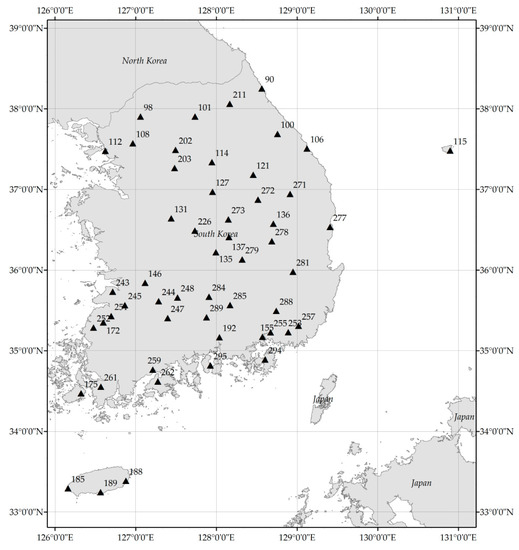
Figure 2.
Geographical location of the weather stations used for hourly mean wind speed data.

Table 1.
Information on the weather stations.
4.1.2. Ten-Minute Mean Wind Speed Data
In the present study, 10-min mean wind speed at a height of 10 m is used. These wind speed data are recorded at 3 meteorological stations located in the United Arab Emirates. Information such as the altitude and the recording period are presented in Table 2. The geographical location of the employed stations is presented in Figure 3. The Al Mirfa and Masdar wind stations are located near the coastline, and the Al Aradh station is located in the foothills. The recording periods of the stations are not long compared with the recording lengths of the hourly mean wind speed data sets. Although the evaluation results for the 10-min mean wind speed data lose generality because of a shortage of observations, the case study for the 10-min mean wind speed data may illustrate the performance of the proposed method at a very fine wind speed temporal resolution.
Table 2.
Information on the stations used to obtain 10-min mean wind speed data.
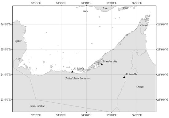
Figure 3.
Geographical location of the weather stations used for 10-min mean wind speed data.
4.2. Test Case Descriptions
4.2.1. Test Cases for Hourly Mean Wind Speed Data
The proposed method temporally downscales the statistical characteristics of the mean wind speed data. Thus, the performance of the proposed method may be different based on the temporal scale used. The performance of the proposed model must be assessed based on the use of wind speed data for different temporal scales. In the current study, two references and ten test cases are used. The target temporal scale of all reference and test cases is hourly. The differences between the test and reference cases are the temporal scales of the mean wind speed data and linear model fitting methods. All reference and test cases are described in Table 3. The goals for all the cases are to obtain the Weibull distribution of hourly mean wind speed data without the use of hourly mean wind speed data. Cases 0–O and 0–W are the reference cases. Because the CRM estimates are obtained by the proposed method using the hourly mean wind speed data, these cases present the best performance of the proposed method. Thus, from the results of cases 0–O and 0–W, we can investigate the maximum performance of the proposed method. The temporal scales of many meteorological observations and estimates are daily to weekly [56,57,58,59]. To assess the applicability of the proposed method for these coarse temporal scales (longer than and equal to daily), cases 1 (weekly) and 2 (daily) are tested. Recently, various wind speed data are provided for sub-daily temporal scales, such as 3-h, 6-h, and 12-h [2,4,60,61,62]. For the sub-daily temporal scales, cases 3 (12-h), 4 (6-h), and 5 (3-h) are tested. The OLS and WLS methods are applied for all the cases to investigate the suitability of the linear model fitting method. The selected cases may well represent various temporal scales of the mean wind speed data.
Table 3.
Description of the test cases for the hourly mean wind speed data.
In the proposed method, four weeks is used as the maximum temporal scale. For example, in the weekly case, the CRMs of one-week, two-week, three-week, and four-week mean wind speed data that are aggregated from the weekly mean wind speed data are used to fit the linear model. In the case of daily mean wind speed data, the CRMs of 1- to 28-day mean wind speed data are used in the linear model fitting. The statistical characteristics of the mean wind speed data for too coarse temporal scales, e.g., one month and two months, may be different from the statistical characteristics of the mean wind speed for fine temporal scales. The use of coarse temporal scale data may lead to worse results when modeling the wind statistics at a fine temporal scale data. Hence, we set four weeks as the maximum temporal scale in the proposed method.
4.2.2. Test Cases for 10-min Mean Wind Speed Data
The target temporal resolution of the test cases in this subsection is 10-min. Hence, these test cases should vary from the test cases for the hourly mean wind speed data. The minimum and maximum temporal resolution of the test cases are hourly and daily (24-h), respectively. Temporal resolutions of 1-, 3-, 6-, 12-, and 24-h are used for the test cases for the 10-min mean wind speed data. Mean wind speed data for the temporal resolution used in the test cases are obtained by aggregating 10-min mean wind speed data for three stations. Because 168-h (weekly case) represents a very coarse resolution compared with 10-min, the 168-h mean wind speed data are not employed as the test case.
5. Results
5.1. Case Study for Hourly Mean Wind Speed Data
5.1.1. Parameter Estimation of the Downscaled Weibull Distribution
The parameters of the downscaled Weibull distributions are obtained by the proposed method for all the stations and cases. The biases between the parameter estimates by the proposed method and original parameter estimates are calculated. The original estimates indicate the parameters obtained by the method of moments from hourly mean wind speed observations. Figure 4 presents boxplots of the biases of the proposed method for estimating parameters of the downscaled Weibull distribution for all the cases. Overall, the proposed method overestimates the scale and shape parameters of the Weibull distribution. The WLS method leads to a better fit than the OLS method for all the cases. The biases of the scale and shape parameters are reduced when the wind speed data temporal scale becomes finer. For the sub-daily cases, i.e., cases 3, 4, and 5, the performance of the proposed method slightly improves when the temporal scale becomes finer. For the scale parameter estimates, the proposed method provides good parameter estimation precision. Additionally, the precision of the shape parameter estimation is good when case 1 is excluded.
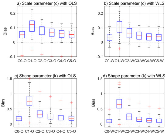
Figure 4.
Boxplots of the Bias of scale (c) and shape (k) parameters of the downscaled Weibull distiribtuion with OLS and WLS methods based on the parameter estimates from the observed Weibull distribution. Note that (a–d) presents boxplots of scale parameter estimates with OLS, scale parameter estiamtes with WLS, shape parameter estimates with OLS, and shape parameter with WLS, respectively.
The ABias values of the proposed method for estimating the Weibull parameters for all the cases are presented in Figure 5. Overall, the ABias results are similar to the Bias results. For the scale parameters, the proposed method with the WLS method provides good estimation performance. Particularly, the medians of the absolute biases for the sub-daily cases are smaller than 0.05. The proposed method provides good performance when estimating the shape parameter for sub-daily cases. When the number of the data point is one, the values of ABias and RMSE are the same. Since each station has one scale parameter and one shape parameter, values of the ABias and RMSEs for each parameter are the same. Because boxplots of RMSE are equivalent to boxplots of the ABias, the boxplots of the RMSE are not illustrated.
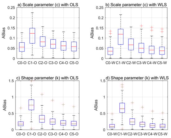
Figure 5.
Boxplots of ABias of scale (c) and shape (k) of the downscaled Weibull distribtuion with the OLS and WLS methods based on the parameter estimates from the observed Weibull distribution. Note that (a), (b), (c) and (d) presents boxplots of scale parameter estimates with OLS, scale parameter estiamtes with WLS, shape parameter estimates with OLS, and shape parameter with WLS, respectively.
The RBiases of the proposed method based on observed parameters for all the cases are presented in Figure 6. The proposed method provides good performance in the scale parameter estimation based on the RBiases. The worst case is case 1, and its RBiases are from −3% to 15% in the scale parameter estimation. The medians of the RBiases for other cases are smaller than 5%. The proposed method overestimates the shape parameter for cases 1 and 2 based on the RBias values. The cases of sub-daily temporal scales (cases 3, 4, and 5) provide relatively good performance for shape parameter estimations. The medians of the RBiases for these cases are smaller than 20%.
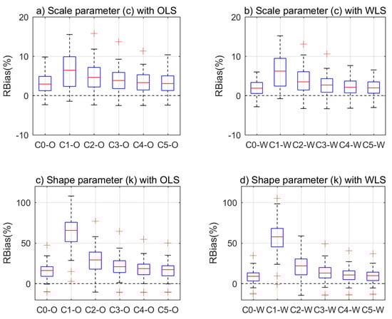
Figure 6.
Boxplots of the RBias(%) of scale (c) and shape (k) parameters of the downscaled Weibull distribution with the OLS and WLS methods based on the parameter estimates from the observed Weibull distribution. Note that (a–d) presents boxplots of scale parameter estimates with OLS, scale parameter estiamtes with WLS, shape parameter estimates with OLS, and shape parameter with WLS, respectively.
Figure 7 presents the ARBias values of the proposed method when downscaling the Weibull parameters for all the cases. Overall, the ARBias results are similar to the RBias results. All ARBias values for the scale parameter estimates are smaller than 15%, and their medians are below 10%. In the case of shape parameter estimation, the use of sub-daily mean wind speed data in the proposed method leads to good precision. The ARBiases of the shape parameter for the sub-daily temporal scales with the WLS method are from 1% to 30%. The weekly and daily cases provide relatively large ARBiases. The ARBias medians for these two cases with the WLS are 60% and 20%.
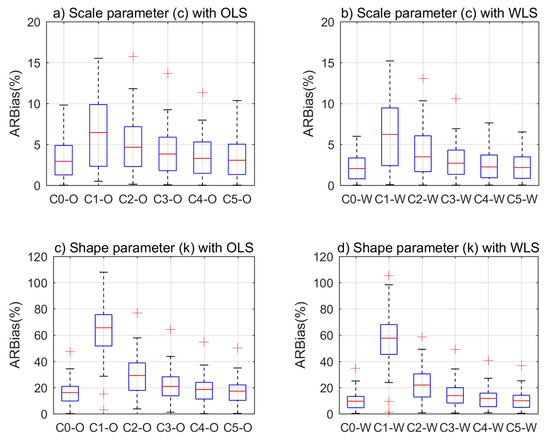
Figure 7.
Boxplots of the ARBias (%) of scale (c) and shape (k) parameters of the downscaled Weibull distribution with the OLS and WLS methods based on the parameter estimates from the observed Weibull distribution. Note that (a–d) presents boxplots of scale parameter estimates with OLS, scale parameter estiamtes with WLS, shape parameter estimates with OLS, and shape parameter with WLS, respectively.
The means for the bias, ABias, RBias, and ARBias of the proposed method for all the cases are presented in Table 4. The WLS method leads to better performance fitting of the linear model than the OLS method based on all employed criteria. The proposed method successfully estimates the scale parameters of the downscaled Weibull distribution. The mean ARBias of the case of daily mean wind speed data for the scale parameter is 5%. The ARBias values of the sub-daily cases with the WLS method are below 15% for the shape parameters. For the weekly and daily cases, the proposed method leads to poor precision when estimating the shape parameter. The mean ARBiases of cases 1 and 2 with the WLS method are approximately 60% and 20%, respectively. Results of RMSE are very similar to the results of ABias.
Table 4.
Means of the evaluation criteria for the downscaled Weibull parameter estimates based on parameter estimates of the observed Weibull distribution of all the stations.
The probability density functions (PDFs) of the downscaled Weibull distributions for all the cases using the WLS method are illustrated in Figure 8 to investigate the differences between the Weibull distribution of the mean wind speed observations and the downscaled Weibull distributions. The downscaled Weibull PDFs successfully reproduced the Weibull PDFs of the hourly mean wind speed observations. When finer temporal scales are used, the downscaled Weibull PDF becomes more similar to the Weibull PDF of the observations. In stations #135, #137, and #252, the downscaled Weibull PDFs of the daily and sub-daily cases are similar to the Weibull PDF of the observations.
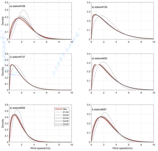
Figure 8.
Probability density functions of the downscaled Weibull distributions with the WLS method for all the cases of stations (a) #108, (b) #135, (c) #137, (d) #252, (e) #255, and (f) #257. The red line indicates the Weibull PDF fitted by the method of moments for the hourly mean wind speed data. The observed distribution (red solid line) indicates the Weibull distribution of hourly wind speed data fitted using the method of moment.
5.1.2. Wind Potential Energy Estimation of the Downscaled Weibull Distribution
The wind speed probability distribution is used to estimate the wind potential energy in regions of interest in the wind energy field. The precision of the parameter estimation as well as the wind potential energy estimation from the downscaled Weibull distribution are important. Thus, in this subsection, the precision of the wind potential energy of the downscaled Weibull distribution is examined.
Figure 9 presents the biases, ABiases, RBiases, and ARBiases of the wind potential energy from the Weibull distribution downscaled by the proposed method for all stations. The downscaled Weibull distribution underestimates the wind potential energy for all the cases based on the wind potential energy from hourly mean wind speed observations. At smaller temporal scales of the wind speed data, the estimation precision of the wind potential energy increases. The precision of the wind potential energy estimation by the proposed method for the weekly and daily cases (cases 1 and 2) is poor based on the RBias and ARBias values. Because boxplots of RMSE are equivalent to boxplots of the ABias, the boxplots of the RMSE are not illustrated in Figure 9.
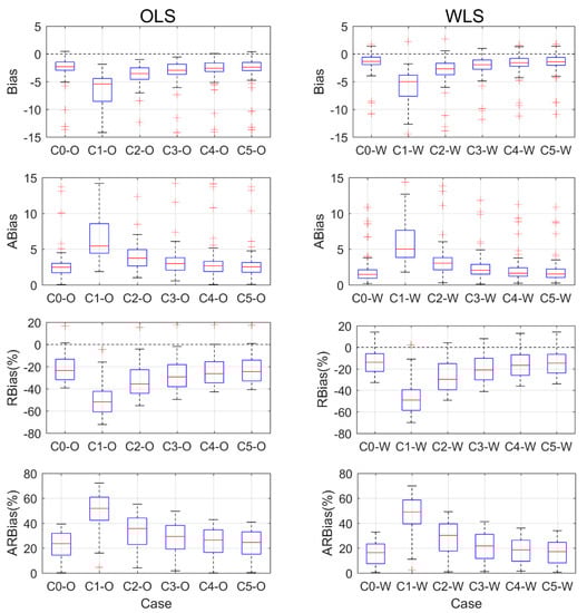
Figure 9.
Boxplots of the bias, ABias, RBias (%), and ARBias (%) of wind potential energy estimates from the downscaled Weibull distribution with the OLS and WLS methods based on the wind potential energy from the observed Weibull distributions. Note that the wind potential energy of station #185 is not presented in bias and ABias. Because the magnitude of the wind potential energy for station #185 is approximately one hundred times the magnitude of the other stations, the boxplot does not properly represent the overall characteristics when the bias and ABias of station #185 are included.
The means of the Bias, ABias, RBias, and ARBias of the wind potential energy estimates by the proposed method for all the cases are presented in Table 5. Based on the means of the Bias and RBias, the Weibull distribution downscaled by the proposed method underestimates the wind potential energy. Overall, the proposed method successfully reproduces the wind potential energy for sub-daily temporal scales such as 3-h, 6-h, and 12-h. The evaluation criteria indicate that 3-h and 6-h mean wind speed data (case 3) can provide a good performance that is nearly equivalent to the reference cases. Results of RMSE for the WPE are different of the results from ABias for the WPE. The OLS method leads to the lower RMSEs than the WLS method. In the case excluding to the station #185, the RMSE of the WPE by OLS and WLS are almost same. From the results, it can be inferred that the WLS is more sensitive to the data having the large variability, e.g., outlier, than the OLS.
Table 5.
Means of the evaluation criteria for the wind potential energy of the downscaled Weibull distributions based on the wind potential energy of the observed Weibull distributions of all the stations. Note that the biases of C3-W, C4-W, and C5-W are positive because the value of the wind potential energy for station #185 is a large positive number. Because the magnitude of the wind potential energy for station #185 is approximately one hundred times the magnitude of the other stations, the mean biases of these cases are shifted. The numbers in brackets indicate the means of the biases without station #185.
5.2. Case Study for 10-min Mean Wind Speed Data
The means of the Bias, ABias, RBias, and ARBias of the proposed method for downscaling the Weibull parameters for all the cases with the 10-min mean wind speed data are presented in Table 6.
Table 6.
Bias, absolute bias, relative bias, and absolute relative bias of the parameter estimates and wind potential energy for the different cases. The presented Bias, ABias, RBias and ARBias values are the mean values for three employed stations. The case indicates the temporal scale of the wind speed data used to obtain the parameters of the Weibull distribution for the 10-min mean wind speed data.
The proposed method underestimates the scale (c) and shape (k) parameters of the downscaled Weibull distribution, which is inconsistent with the results of the case study for the hourly mean wind speed data, where the method leads to overestimations when estimating the parameters of the downscaled Weibull distribution. The proposed method provides very high precision when estimating the scale parameters of the downscaled Weibull distribution. The precision of the shape parameter estimation is worse than the precision of the scale parameter estimation. Overall, the ARBiases for the scale and shape parameters are 1% and 10%, respectively. The proposed method leads to an underestimation in the wind potential estimation. For the sub-daily cases (1-, 3-, 6-, and 12-h cases), the ARBiases of the wind potential energy are smaller than 14%. Very large ARBiases are observed for the 24-h case. Results of RMSE are very similar to the results of ABias. The use of the OLS method leads to a better performance than the WLS method for the case study with 10-min mean wind speed data. The best results are observed in the 12-h case. According to the results of the case study for the hourly mean wind speed data, the 1-h case may provide the best performance because the mean wind speed data with finer temporal resolution leads to better performance in parameter and wind potential energy estimation. However, these results are not observed in the results of the case study with 10-min mean wind speed data. These discrepancies may be related to the small number of stations used.
Figure 10 presents the observed and downscaled Weibull PDFs with the OLS and WLS methods for six stations. The proposed method successfully reproduces the Weibull PDF of the 10-min mean wind speed observations for the Al Aradh and Al Mirfa stations. For the Al Aradh station, the Weibull PDFs downscaled by 1-, 3-, 6-, and 12-h mean wind speed data successfully reproduce the Weibull PDF of the 10-min mean wind speed observations.
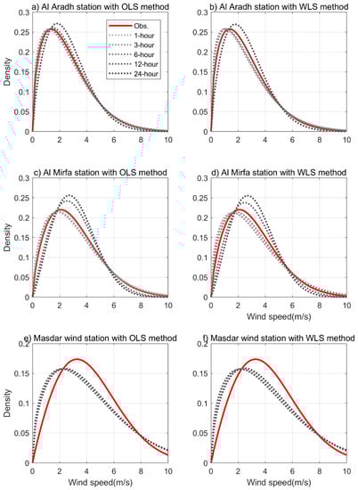
Figure 10.
Observed and downscaled Weibull PDFs with the OLS and WLS methods for six stations with Weibull PDF observations. Note that the target temporal resolution of the downscaling method is 10 min. The red line indicates the Weibull PDF that is fitted by the method of moments for 10-min mean wind speed data. The observed distribution (red solid line) indicates the Weibull distribution of 10-min wind speed data fitted using the method of moment. Note that (a), (b), (c), (d), (e), and (f) present the pdfs of Al Aradh with OLS, Al Aradh with WLS, Al Mirfa with OLS, Al Mirfa with WLS, Masdar wind station with OLS, and Masdar wind station with WLS, respectively.
The 1-, 3-, and 6-h cases successfully reproduce the observed Weibull PDF of the 10-min mean wind speed data. For the Masdar wind station, the proposed method does not present a good performance when downscaling the wind speed distribution. The downscaling results of the OLS and WLS methods are similar. The performance of the proposed method with the OLS method is better than that with the WLS method for the 10-min mean wind speed data.
6. Discussion
The Weibull parameter estimation precision of the proposed method in the current study varies depending on the temporal scale of the mean wind speed data. In the scale parameter estimation of the downscaled Weibull distribution, the proposed method leads to good precision for most of the cases except for case 1 (weekly case). Thus, the proposed method can be used to estimate the scale parameter of the hourly wind speed Weibull distribution when the daily mean wind speed data are available. However, the estimation precision of the shape parameter for the downscaled Weibull distribution is good for the sub-daily cases (3-h, 6-h, and 12-h cases) based on the employed evaluation criteria. These results indicate that at least daily mean wind speed data are required to obtain reliable parameter estimates of the downscaled Weibull distribution from the proposed method.
Additionally, the evaluation criteria results show that the performance of the proposed method worsens when the temporal scales of the mean wind speed data become coarser. These results indicate that the mean wind speed data with a temporal scale close to fine scale can provide considerable information for downscaling the Weibull distribution. Additionally, although linear correlations between the log of the CRM and the log of the temporal scale are very high, the fine temporal scale data may be more similar to hourly mean wind speed data because their relationships are not perfectly linear.
A validation of the proposed method is carried out to investigate the performance of the proposed method in an unused data set. In the validation, the original dataset is divided into two data sets: training and test datasets. Half of the data points in the original dataset are randomly selected as the training dataset. The remaining of data points become the test datasets. The proposed method is applied to the training data set to estimate parameters of the downscaled Weibull distribution for the hourly wind speed data. The parameter estimates of the downscaled Weibull distribution are compared to the Weibull parameter estimates of the hourly wind speed observations in the test dataset. The validation results are presented in Table 7. The results of the validation are very similar to the results of the evaluation presented in Table 4. This result supports the conclusion that the proposed method provides consistent performances in evaluation and validation for downscaling wind speed distribution. It can be inferred that the proposed method will produce consistent results for an unused dataset such as future wind speed data.
Table 7.
Means of the evaluation criteria for the downscaled Weibull parameter estimates based on parameter estimates of the observed Weibull distribution of all the stations from the test period.
The parameters of the Weibull distribution using raw wind speed data with different temporal scales are estimated and compared with the Weibull parameter estimates using the proposed downscaling method. Table 8 presents the results for the Weibull parameter estimates using the raw wind speed data with different temporal resolutions based on the parameter estimates of the Weibull distribution for hourly wind speed data at all the stations. The Weibull parameter estimates using the proposed downscaling method are closer to the Weibull parameters of hourly wind speed data than those of raw wind speed data except for 3-h wind speed data. For the case of 3-h wind speed data, the downscaling method does not include large values in estimating the Weibull parameters of the hourly wind speed data. This is natural outcome. Because finer temporal wind speed data is definitely more similar to the hourly wind speed data, the downscaling method may not provide a large improvement in parameter estimation of the Weibull distribution. Overall, the proposed method leads to an improvement in parameter estimation. Based on the results presented in Table 7, wind speed data with coarse temporal resolution, i.e., is longer than 3-h, should be used with the proposed downscaling method for parameter estimation of Weibull distribution. Hence, the proposed method in the current study is a good option for estimating the parameters of the Weibull distribution and conducting a preliminary wind power potential assessment in areas where the mean wind speed observations of high temporal resolution are not available.
Table 8.
Means of the evaluation criteria for the Weibull parameter estimates by the raw wind speed data with different temporal scale based on the parameter estimates of the Weibull distribution for hourly wind speed data at all the stations. Note that the underline indicates that the accuracy of Weibull parameter estimates from the raw data is superior to the Weibull parameter estimates by the downscaling method.
The Weibull PDFs downscaled by the coarse temporal scales are less skewed than those of the cases at fine temporal scales. The mean wind speed data at a coarse temporal scale are averaged from the mean wind speed data at a fine temporal scale. The very large and small mean wind speed data that introduce skewness in the distribution shape may be removed because of the averaging process. Thus, mean wind speed data with a coarse temporal resolution shows a less skewed distribution shape than the data at a fine temporal scale. The temporal downscaling of the mean wind speed data is a method of reproducing the skewness and variance of fine temporal scale wind speed data. The results of the Weibull PDF comparisons indicate that the Weibull PDFs downscaled by the proposed method using the daily wind speed data successfully reproduce the distributional characteristics of the Weibull distribution from 10-min and hourly mean wind speed observations for the stations presented in Figure 8 and Figure 10.
The proposed method can provide the downscaled Weibull distribution that is much more similar to the 10-min or hourly Weibull distribution than the use of raw data when temporal scale of raw wind speed data is longer than 3-h. The use of the proposed method has to be considered in the wind potential energy assessment using wind speed data of the coarse temporal scale (longer than 6-h). However, the estimation precision of the method proposed in the current study for wind potential energy varies depending on the temporal scale and is worse than the precision of the Weibull parameter estimation because the errors in the Weibull parameter estimation propagate to the wind potential energy estimation. Additionally, the errors may be introduced via inaccurate shape parameter estimations because of the relatively worse performance of the shape parameter estimation. Six hours may represent a threshold in the proposed model for the temporal scale to obtain relatively accurate wind potential energy because the performance of the proposed method for cases 4 and 5 is close to the performance for the reference cases. The proposed method is recommended to improve accurary
The results of the wind potential energy estimation indicate that precise parameter estimations are required to obtain precise wind potential energy estimations from the Weibull distribution. Although the parameter estimates are relatively precise, such as for the daily case, the wind potential estimation precision may be poor. Additionally, the performance of the reference cases represents the maximum capacity of the proposed method to downscale the Weibull distribution of the mean wind speed data, and the mean ARBias of the reference case (case 0–W) is 15%, which is not small enough to be neglected in the wind potential energy estimation. Thus, the proposed method should be used only for approximate estimations of wind potential energy.
Many regions do not have fine temporal resolution wind speed data, e.g., offshore area, and developing countries areas. Recent advanced climate models allow the simulation of wind speed data for regions where the resolution of observation is poor or there is no observation. Therefore, to obtain the wind speed data with fine temporal resolution, climate models are often used [2,3,9,20]. However, the climate models require very large computation resources to simulate the wind speed data at fine temporal and spatial resolutions (for example, minute and 10-min resolutions). Due to a requirement of large computation resources, hourly or daily resolution is usually used as the temporal resolution [16,18,24,63]. The statistical downscaling method can be an alternative to the climate model. The proposed method in the current study is to downscale the wind speed distribution instead of downscaling the wind speed data. Because the proposed temporal downscaling method can provide a more accurate estimation of the wind speed distribution using coarse temporal wind speed data, wind power potential estimation from the proposed method in these regions may be more accurate than the use of raw wind speed data with coarse temporal resolution. For example, outputs of the climate model can be downscaled again using the proposed method. Applying the statistical downscaling method to the outputs of the climate models is a popular approach to obtain data with fine temporal and spatial resolutions in the climate change field [5,64,65,66,67]. Additionally, the proposed method can be employed to remote wind speed observations such as QuikSCAT and OSCAT. Due to the orbit of satellites, the observing frequency of remote sensing data is weekly or daily [58,68]. The proposed method allows us to obtain a more accurate estimation of the wind speed distribution from the remote sensing data. Therefore, the proposed method can enhance our capacity to estimate the wind speed distribution and increase the availability and usage of wind speed data with a coarse temporal scale in an assessment of wind power potential.
The scaling property is generally used as an index representing the structure of data for the different scales. In the current study, the distribution of wind speed data was temporally downscaled by the scaling property representing the temporal structure of the wind speed data. The characteristics of the scaling property can be expressed by a scaling exponent. The scaling exponent was not explained in the current study because this value was not necessary to downscale the distribution of wind speed data. More detailed information and a definition of the scaling exponent can be found in [69,70,71]. The spatial distribution of the scaling exponents for the stations used in South Korea is analyzed to investigate the locality of the scaling property in wind speed data (the spatial distribution of the scaling exponents is not shown). The spatial distribution of the scaling exponents shows that they vary depending on the location of the stations. Because the characteristics of wind speed data may vary based on local atmospheric characteristics, this result is natural. However, the scaling exponents for certain stations are very different from those of nearby stations. For example, the scaling exponents of certain stations in urban areas and islands are different from those of nearby stations, which supports the strong effect of wind shear or roughness on the scaling exponents of the wind speed data. The drastic difference between two nearby stations may come from the terrain complexity. The terrain shape and complexity can influence the wind shear [72,73,74]. The scaling exponent can also be affected by the terrain complexity. Hence, characteristics of the terrain complexity at an area of the interest affect the spatial interpolation of the scaling exponent for wind speed data.
In the scaling property, the distribution of the data at different scales may be equivalent based on a power law relationship with the scaling exponent [75,76,77]. This concept of the scaling property is similar to a power law relationship for a wind profile, although it is not exactly the same because the distributions are the same while the data are not. The power law relationship for the wind profile has been widely used to estimate the wind speed at different heights [78,79,80,81,82,83]. When the wind profile is assumed to follow the power law, the proposed method can be employed for downscaling the distribution of wind speeds near the ground. In other words, the proposed method may not be appropriate for wind speeds at different heights when the wind profile follows other laws, such as log-linear and logarithmic laws. Additionally, because the power law and scaling property laws were derived based on empirical relationships, the applicability of the proposed method for the wind speed at different heights should be evaluated.
7. Conclusions and Recommendations
A novel temporal downscaling method for wind speed Weibull distributions is proposed in the current study. The performance and applicability of the proposed method are assessed for the mean wind speed data of several temporal scales in South Korea based on the employed evaluation criteria. In the current study, the following conclusions are reached.
- The novel method provides the downscaled Weibull distribution of hourly mean wind speed data using wind statistics at coarse temporal scales, such as 3-h, 6-h, 12-h, and daily scales. Particularly, the use of sub-daily mean wind speed data in the downscaling of the wind speed Weibull distribution leads to good estimation precision. The proposed method provides a good approximation of the hourly mean wind speed Weibull distribution for wind power potential estimations in regions where hourly wind speed data are unavailable.
- The proposed method successfully estimates the scale parameters of the downscaled Weibull distribution for hourly mean wind speed. The precision of the shape parameter estimation by the proposed method is relatively worse than that of the scale parameter estimation. The proposed method presents a good performance when estimating the shape parameter in the cases of sub-daily temporal scales. The proposed method can be used to obtain the downscaled Weibull distribution in the case of a daily temporal scale based on the Weibull parameter estimation, although the performance of the proposed method for this case is poor. However, because the proposed method leads to a poor performance in the weekly case, at least a daily wind speed temporal scale should be used to estimate the parameters of the Weibull distribution for hourly mean wind speed.
- The Weibull distribution downscaled by the proposed method successfully reproduces the wind power density based on the wind potential energy estimation. For the cases of sub-daily temporal scales, the proposed method provides a good approximate wind potential energy of hourly mean wind speed data without using the hourly mean wind speed data. The proposed method presents poor precision in the cases of weekly and daily temporal scales, which is similar to the results of the parameter estimation. Thus, for estimating the downscaled wind potential energy, the mean wind speed data of sub-daily temporal scales should be used in the proposed method. In addition, the results of the proposed method may be used to assess the approximate wind potential energy in regions that do not have mean wind speed observations at a fine temporal scale.
- The proposed downscaling method gives an improvement in estimating parameters of Weibull distribution for wind speed data. The precision of Weibull parameter estimation by the proposed method is superior to the precision of the parameter estimation for raw wind speed data without use of the downscaling method when the temporal scale of the used wind speed data is longer than 3-h. For the case of 3-h mean wind speed data, the proposed method shows comparable performance to parameter estimation for the raw wind speed data.
- The WLS method leads to a better performance than the OLS method. Based on all employed evaluation criteria, the WLS method is superior to the OLS method for precisely fitting a linear model via the proposed method, especially for the CRM of the hourly mean wind speed data. The WLS method is recommended for fitting a linear model via the proposed method.
The proposed downscaling method in the present study has considerable potential to be extended and improved. Because the proposed method temporally downscales statistical characteristics (moments) of the mean wind speed data, it can be employed for any frequency distribution models for which the method of moments can be used, and these features may represent good topics for further research on the proposed method. Additionally, because this method can be applied for time series data for other renewable sources, e.g., solar radiation and wave heights, investigating its applicability to other renewable sources that use time data would represent a good further research topic [84,85,86,87,88,89].
Acknowledgments
This work was supported by the National Research Foundation of Korea (NRF) grant funded by the Korea government (Ministry of Science, ICT & Future Planning) (No. 2017R1A2B4009338).
Author Contributions
Ju-Young Shin, Changsam Jeong, and Jun-Haeng Heo conceived and designed the experiments; Ju-Young Shin and Changsam Jeong performed the experiments; Ju-Young Shin and Changsam Jeong analyzed the data; Ju-Young Shin contributed reagents/materials/analysis tools; Ju-Young Shin and Jun-Haeng Heo wrote the paper.
Conflicts of Interest
The authors declare no conflict of interest. The founding sponsors had no role in the design of the study; in the collection, analyses, or interpretation of data; in the writing of the manuscript, and in the decision to publish the results.
References
- Kent, E.C.; Fangohr, S.; Berry, D.I. A comparative assessment of monthly mean wind speed products over the global ocean. Int. J. Climatol. 2012, 33, 2520–2541. [Google Scholar] [CrossRef]
- Chadee, X.T.; Clarke, R.M. Large-scale wind energy potential of the caribbean region using near-surface reanalysis data. Renew. Sustain. Energy Rev. 2014, 30, 45–58. [Google Scholar] [CrossRef]
- Cannon, D.J.; Brayshaw, D.J.; Methven, J.; Coker, P.J.; Lenaghan, D. Using reanalysis data to quantify extreme wind power generation statistics: A 33 year case study in great britain. Renew. Energy 2015, 75, 767–778. [Google Scholar] [CrossRef]
- Gadad, S.; Deka, P.C. Offshore wind power resource assessment using oceansat-2 scatterometer data at a regional scale. Appl. Energy 2016, 176, 157–170. [Google Scholar] [CrossRef]
- Lee, T.; Park, T. Nonparametric temporal downscaling with event-based population generating algorithm for rcm daily precipitation to hourly: Model development and performance evaluation. J. Hydrol. 2017, 547, 498–516. [Google Scholar] [CrossRef]
- Ben Alaya, M.A.; Chebana, F.; Ouarda, T.B.M.J. Multisite and multivariable statistical downscaling using a gaussian copula quantile regression model. Clim. Dyn. 2016, 47, 1383–1397. [Google Scholar] [CrossRef]
- Olsson, J.; Willén, U.; Kawamura, A. Downscaling extreme short-term regional climate model precipitation for urban hydrological applications. Hydrol. Res. 2012, 43, 341–351. [Google Scholar] [CrossRef]
- Fujihara, Y.; Tanaka, K.; Watanabe, T.; Nagano, T.; Kojiri, T. Assessing the impacts of climate change on the water resources of the seyhan river basin in turkey: Use of dynamically downscaled data for hydrologic simulations. J. Hydrol. 2008, 353, 33–48. [Google Scholar] [CrossRef]
- Lorenz, T.; Barstad, I. A dynamical downscaling of era-interim in the north sea using wrf with a 3 km grid-for wind resource applications. Wind Energy 2016, 19, 1945–1959. [Google Scholar] [CrossRef]
- Wilks, D.S.; Wilby, R.L. The weather generation game: A review of stochastic weather models. Prog. Phys. Geogr. 1999, 23, 329–357. [Google Scholar] [CrossRef]
- Hewitson, B.C.; Crane, R.G. Climate downscaling: Techniques and application. Clim. Res. 1996, 7, 85–95. [Google Scholar] [CrossRef]
- Salameh, T.; Drobinski, P.; Vrac, M.; Naveau, P. Statistical downscaling of near-surface wind over complex terrain in southern france. Meteorol. Atmos. Phys. 2008, 103, 253–265. [Google Scholar] [CrossRef]
- Howard, T.; Clark, P. Correction and downscaling of nwp wind speed forecasts. Meteorol. Appl. 2007, 14, 105–116. [Google Scholar] [CrossRef]
- Monahan, A.H. Can we see the wind? Statistical downscaling of historical sea surface winds in the subarctic northeast pacific. J. Clim. 2012, 25, 1511–1528. [Google Scholar] [CrossRef]
- Gaitan, C.F.; Cannon, A.J. Validation of historical and future statistically downscaled pseudo-observed surface wind speeds in terms of annual climate indices and daily variability. Renew. Energy 2013, 51, 489–496. [Google Scholar] [CrossRef]
- Winstral, A.; Jonas, T.; Helbig, N. Statistical downscaling of gridded wind speed data using local topography. J. Hydrometeorol. 2017, 18, 335–348. [Google Scholar] [CrossRef]
- Kirchmeier, M.C.; Lorenz, D.J.; Vimont, D.J. Statistical downscaling of daily wind speed variations. J. Appl. Meteorol. Climatol. 2014, 53, 660–675. [Google Scholar] [CrossRef]
- Manor, A.; Berkovic, S. Bayesian inference aided analog downscaling for near-surface winds in complex terrain. Atmos. Res. 2015, 164, 27–36. [Google Scholar] [CrossRef]
- Huang, H.-Y.; Capps, S.B.; Huang, S.-C.; Hall, A. Downscaling near-surface wind over complex terrain using a physically-based statistical modeling approach. Clim. Dyn. 2014, 44, 529–542. [Google Scholar] [CrossRef]
- Horvath, K.; Bajić, A.; Ivatek-Šahdan, S. Dynamical downscaling of wind speed in complex terrain prone to bora-type flows. J. Appl. Meteorol. Climatol. 2011, 50, 1676–1691. [Google Scholar] [CrossRef]
- Michelangeli, P.A.; Vrac, M.; Loukos, H. Probabilistic downscaling approaches: Application to wind cumulative distribution functions. Geophys. Res. Lett. 2009, 36. [Google Scholar] [CrossRef]
- Pryor, S.C.; Barthelmie, R.J.; Kjellström, E. Potential climate change impact on wind energy resources in northern europe: Analyses using a regional climate model. Clim. Dyn. 2005, 25, 815–835. [Google Scholar] [CrossRef]
- Pryor, S.C.; Schoof, J.T.; Barthelmie, R.J. Empirical downscaling of wind speed probability distributions. J. Geophys. Res. Atmos. 2005, 110. [Google Scholar] [CrossRef]
- Devis, A.; van Lipzig, N.P.M.; Demuzere, M. A new statistical approach to downscale wind speed distributions at a site in northern europe. J. Geophys. Res. Atmos. 2013, 118, 2272–2283. [Google Scholar] [CrossRef]
- Kumar, J.; Brooks, B.-G.J.; Thornton, P.E.; Dietze, M.C. Sub-daily statistical downscaling of meteorological variables using neural networks. Procedia Comput. Sci. 2012, 9, 887–896. [Google Scholar] [CrossRef]
- Guo, Z.; Chang, C.; Wang, R. A novel method to downscale daily wind statistics to hourly wind data for wind erosion modelling. In Geo-Informatics in Resource Management and Sustainable Ecosystem, Proceedings of the Third International Conference, Grmse 2015, Wuhan, China, 16–18 October 2015; revised selected papers; Bian, F., Xie, Y., Eds.; Springer: Berlin/Heidelberg, Germany, 2016; pp. 611–619. [Google Scholar]
- Gupta, V.K.; Waymire, E. Multiscaling properties of spatial rainfall and river flow distributions. J. Geophys. Res. Atmos. 1990, 95, 1999–2009. [Google Scholar] [CrossRef]
- Gupta, V.K.; Mesa, O.J.; Dawdy, D.R. Multiscaling theory of flood peaks: Regional quantile analysis. Water Resour. Res. 1994, 30, 3405–3421. [Google Scholar] [CrossRef]
- Basu, B.; Srinivas, V.V. A recursive multi-scaling approach to regional flood frequency analysis. J. Hydrol. 2015, 529, 373–383. [Google Scholar] [CrossRef]
- Yonghe, L.; Kexin, Z.; Wanchang, Z.; Yuehong, S.; Hongqin, P.; Jinming, F. Multifractal analysis of 1-min summer rainfall time series from a monsoonal watershed in eastern china. Theor. Appl. Climatol. 2013, 111, 37–50. [Google Scholar] [CrossRef]
- Langousis, A.; Veneziano, D.; Furcolo, P.; Lepore, C. Multifractal rainfall extremes: Theoretical analysis and practical estimation. Chaos Solitons Fractals 2009, 39, 1182–1194. [Google Scholar] [CrossRef]
- Veneziano, D.; Lepore, C. The scaling of temporal rainfall. Water Resour. Res. 2012, 48, W08516. [Google Scholar] [CrossRef]
- Fac-Beneda, J. Fractal structure of the kashubian hydrographic system. J. Hydrol. 2013, 488, 48–54. [Google Scholar] [CrossRef]
- Huang, H.-H.; Puente, C.E.; Cortis, A.; Fernández Martínez, J.L. An effective inversion strategy for fractal–multifractal encoding of a storm in boston. J. Hydrol. 2013, 496, 205–216. [Google Scholar] [CrossRef]
- Langousis, A.; Carsteanu, A.; Deidda, R. A simple approximation to multifractal rainfall maxima using a generalized extreme value distribution model. Stoch. Environ. Res. Risk Assess. 2013, 27, 1525–1531. [Google Scholar] [CrossRef]
- Kim, J.-C.; Jung, K. Fractal tree analysis of drainage patterns. Water Resour. Manag. 2015, 29, 1217–1230. [Google Scholar] [CrossRef]
- Alipour, M.H.; Rezakhani, A.T.; Shamsai, A. Seasonal fractal-scaling of floods in two u.S. Water resources regions. J. Hydrol. 2016, 540, 232–239. [Google Scholar] [CrossRef]
- Kavasseri, R.G.; Nagarajan, R. A multifractal description of wind speed records. Chaos Solitons Fractals 2005, 24, 165–173. [Google Scholar] [CrossRef]
- Chang, T.-P.; Ko, H.-H.; Liu, F.-J.; Chen, P.-H.; Chang, Y.-P.; Liang, Y.-H.; Jang, H.-Y.; Lin, T.-C.; Chen, Y.-H. Fractal dimension of wind speed time series. Appl. Energy 2012, 93, 742–749. [Google Scholar] [CrossRef]
- Telesca, L.; Lovallo, M.; Kanevski, M. Power spectrum and multifractal detrended fluctuation analysis of high-frequency wind measurements in mountainous regions. Appl. Energy 2016, 162, 1052–1061. [Google Scholar] [CrossRef]
- Piacquadio, M.; de la Barra, A. Multifractal analysis of wind velocity data. Energy Sustain. Dev. 2014, 22, 48–56. [Google Scholar] [CrossRef]
- Koçak, K. Examination of persistence properties of wind speed records using detrended fluctuation analysis. Energy 2009, 34, 1980–1985. [Google Scholar] [CrossRef]
- Telesca, L.; Lovallo, M. Analysis of the time dynamics in wind records by means of multifractal detrended fluctuation analysis and the fisher–shannon information plane. J. Stat. Mech. Theory Exp. 2011, 2011, P07001. [Google Scholar] [CrossRef]
- Costa Rocha, P.A.; de Sousa, R.C.; de Andrade, C.F.; da Silva, M.E.V. Comparison of seven numerical methods for determining weibull parameters for wind energy generation in the northeast region of brazil. Appl. Energy 2012, 89, 395–400. [Google Scholar] [CrossRef]
- Carta, J.A.; Ramírez, P.; Velázquez, S. A review of wind speed probability distributions used in wind energy analysis: Case studies in the canary islands. Renew. Sustain. Energy Rev. 2009, 13, 933–955. [Google Scholar] [CrossRef]
- Chang, T.P. Performance comparison of six numerical methods in estimating weibull parameters for wind energy application. Appl. Energy 2011, 88, 272–282. [Google Scholar] [CrossRef]
- Akdağ, S.A.; Dinler, A. A new method to estimate weibull parameters for wind energy applications. Energy Convers. Manag. 2009, 50, 1761–1766. [Google Scholar] [CrossRef]
- Akdağ, S.A.; Güler, Ö. A novel energy pattern factor method for wind speed distribution parameter estimation. Energy Convers. Manag. 2015, 106, 1124–1133. [Google Scholar] [CrossRef]
- Celik, A.N. A statistical analysis of wind power density based on the weibull and rayleigh models at the southern region of turkey. Renew. Energy 2004, 29, 593–604. [Google Scholar] [CrossRef]
- Sulaiman, M.Y.; Akaak, A.M.; Wahab, M.A.; Zakaria, A.; Sulaiman, Z.A.; Suradi, J. Wind characteristics of oman. Energy 2002, 27, 35–46. [Google Scholar] [CrossRef]
- Wais, P. A review of weibull functions in wind sector. Renew. Sustain. Energy Rev. 2017, 70, 1099–1107. [Google Scholar] [CrossRef]
- Zhou, Y.; Smith, S.J. Spatial and temporal patterns of global onshore wind speed distribution. Environ. Res. Lett. 2013, 8, 034029. [Google Scholar] [CrossRef]
- Fyrippis, I.; Axaopoulos, P.J.; Panayiotou, G. Wind energy potential assessment in naxos island, greece. Appl. Energy 2010, 87, 577–586. [Google Scholar] [CrossRef]
- Shin, J.-Y.; Ouarda, T.B.M.J.; Lee, T. Heterogeneous mixture distributions for modeling wind speed, application to the uae. Renew. Energy 2016, 91, 40–52. [Google Scholar] [CrossRef]
- Ouarda, T.B.M.J.; Charron, C.; Shin, J.-Y.; Marpu, P.R.; Al-Mandoos, A.H.; Al-Tamimi, M.H.; Ghedira, H.; Al Hosary, T.N. Probability distributions of wind speed in the uae. Energy Convers. Manag. 2015, 93, 414–434. [Google Scholar] [CrossRef]
- Celik, A.N. Energy output estimation for small-scale wind power generators using weibull-representative wind data. J. Wind Eng. Ind. Aerodyn. 2003, 91, 693–707. [Google Scholar] [CrossRef]
- Archer, C.L.; Jacobson, M.Z. Evaluation of global wind power. J. Geophys. Res. Atmos. 2005, 110, D12110. [Google Scholar] [CrossRef]
- Nagababu, G.; Simha, R.R.; Naidu, N.K.; Kachhwaha, S.S.; Savsani, V. Application of oscat satellite data for offshore wind power potential assessment of india. Energy Procedia 2016, 90, 89–98. [Google Scholar] [CrossRef]
- Chandel, S.S.; Ramasamy, P.; Murthy, K.S.R. Wind power potential assessment of 12 locations in western himalayan region of india. Renew. Sustain. Energy Rev. 2014, 39, 530–545. [Google Scholar] [CrossRef]
- Naizghi, M.S.; Ouarda, T.B.M.J. Teleconnections and analysis of long-term wind speed variability in the uae. Int. J. Climatol. 2017, 37, 230–248. [Google Scholar] [CrossRef]
- Waewsak, J.; Landry, M.; Gagnon, Y. Offshore wind power potential of the gulf of thailand. Renew. Energy 2015, 81, 609–626. [Google Scholar] [CrossRef]
- Langodan, S.; Viswanadhapalli, Y.; Dasari, H.P.; Knio, O.; Hoteit, I. A high-resolution assessment of wind and wave energy potentials in the red sea. Appl. Energy 2016, 181, 244–255. [Google Scholar] [CrossRef]
- González-Aparicio, I.; Monforti, F.; Volker, P.; Zucker, A.; Careri, F.; Huld, T.; Badger, J. Simulating european wind power generation applying statistical downscaling to reanalysis data. Appl. Energy 2017, 199, 155–168. [Google Scholar] [CrossRef]
- Sunyer, M.A.; Madsen, H.; Ang, P.H. A comparison of different regional climate models and statistical downscaling methods for extreme rainfall estimation under climate change. Atmos. Res. 2012, 103, 119–128. [Google Scholar] [CrossRef]
- Onyutha, C.; Tabari, H.; Rutkowska, A.; Nyeko-Ogiramoi, P.; Willems, P. Comparison of different statistical downscaling methods for climate change rainfall projections over the lake victoria basin considering cmip3 and cmip5. J. Hydro-Environ. Res. 2016, 12, 31–45. [Google Scholar] [CrossRef]
- Mamalakis, A.; Langousis, A.; Deidda, R.; Marrocu, M. A parametric approach for simultaneous bias correction and high-resolution downscaling of climate model rainfall. Water Resour. Res. 2017, 53, 2149–2170. [Google Scholar] [CrossRef]
- Zhu, X.; Qiu, X.; Zeng, Y.; Ren, W.; Tao, B.; Pan, H.; Gao, T.; Gao, J. High-resolution precipitation downscaling in mountainous areas over china: Development and application of a statistical mapping approach. Int. J. Climatol. 2018, 38, 77–93. [Google Scholar] [CrossRef]
- Jiang, D.; Zhuang, D.; Huang, Y.; Wang, J.; Fu, J. Evaluating the spatio-temporal variation of china’s offshore wind resources based on remotely sensed wind field data. Renew. Sustain. Energy Rev. 2013, 24, 142–148. [Google Scholar] [CrossRef]
- Soltani, S.; Helfi, R.; Almasi, P.; Modarres, R. Regionalization of rainfall intensity-duration-frequency using a simple scaling model. Water Resour. Manag. 2017, 31, 4253–4273. [Google Scholar] [CrossRef]
- Menabde, M.; Seed, A.; Pegram, G. A simple scaling model for extreme rainfall. Water Resour. Res. 1999, 35, 335–339. [Google Scholar] [CrossRef]
- Burlando, P.; Rosso, R. Scaling and muitiscaling models of depth-duration-frequency curves for storm precipitation. J. Hydrol. 1996, 187, 45–64. [Google Scholar] [CrossRef]
- Irwin, J.S. A theoretical variation of the wind profile power-law exponent as a function of surface roughness and stability. Atmos. Environ. 1979, 13, 191–194. [Google Scholar] [CrossRef]
- Gualtieri, G.; Secci, S. Wind shear coefficients, roughness length and energy yield over coastal locations in southern italy. Renew. Energy 2011, 36, 1081–1094. [Google Scholar] [CrossRef]
- Ray, M.; Rogers, A.; McGowan, J. Analysis of Wind Shear Models and Trends in Different Terrains; Renewable Energy Research Laboratory, Department of Mechanical & Industrial Engineering, University of Massachusetts: Amherst, MA, USA, 2006; Volume 1003. [Google Scholar]
- Galmarini, S.; Steyn, D.G.; Ainslie, B. The scaling law relating world point-precipitation records to duration. Int. J. Climatol. 2004, 24, 533–546. [Google Scholar] [CrossRef]
- Jung, Y.; Shin, J.-Y.; Ahn, H.; Heo, J.-H. The spatial and temporal structure of extreme rainfall trends in south korea. Water 2017, 9, 809. [Google Scholar] [CrossRef]
- Zhang, H.; Fraedrich, K.; Zhu, X.; Blender, R.; Zhang, L. World’s greatest observed point rainfalls: Jennings (1950) scaling law. J. Hydrometeorol. 2013, 14, 1952–1957. [Google Scholar] [CrossRef]
- Wagner, R.; Courtney, M.; Gottschall, J.; Lindelöw-Marsden, P. Accounting for the speed shear in wind turbine power performance measurement. Wind Energy 2011, 14, 993–1004. [Google Scholar] [CrossRef]
- Sonia, W.; Julie, K.L. Atmospheric stability affects wind turbine power collection. Environ. Res. Lett. 2012, 7, 014005. [Google Scholar]
- Holtslag, M.C.; Bierbooms, W.A.A.M.; van Bussel, G.J.W. Extending the diabatic surface layer wind shear profile for offshore wind energy. Renew. Energy 2017, 101, 96–110. [Google Scholar] [CrossRef]
- Gualtieri, G.; Secci, S. Comparing methods to calculate atmospheric stability-dependent wind speed profiles: A case study on coastal location. Renew. Energy 2011, 36, 2189–2204. [Google Scholar] [CrossRef]
- Liu, Y.; Chen, D.; Yi, Q.; Li, S. Wind profiles and wave spectra for potential wind farms in south china sea. Part i: Wind speed profile model. Energies 2017, 10, 125. [Google Scholar] [CrossRef]
- Şen, Z.; Altunkaynak, A.; Erdik, T. Wind velocity vertical extrapolation by extended power law. Adv. Meteorol. 2012, 2012, 178623. [Google Scholar] [CrossRef]
- Alobaidi, M.H.; Marpu, P.R.; Ouarda, T.B.M.J.; Ghedira, H. Mapping of the solar irradiance in the uae using advanced artificial neural network ensemble. IEEE J. Sel. Top. Appl. Earth Obs. Remote Sens. 2014, 7, 3668–3680. [Google Scholar] [CrossRef]
- Ouarda, T.B.M.J.; Charron, C.; Marpu, P.R.; Chebana, F. The generalized additive model for the assessment of the direct, diffuse and global solar irradiances using seviri images, with application to the uae. J. Sel. Top. Appl. Earth Obs. Remote Sens. 2016, in press. [Google Scholar] [CrossRef]
- Fortuna, L.; Nunnari, G.; Nunnari, S. A new fine-grained classification strategy for solar daily radiation patterns. Pattern Recognit. Lett. 2016, 81, 110–117. [Google Scholar] [CrossRef]
- Wu, Y.; Randell, D.; Christou, M.; Ewans, K.; Jonathan, P. On the distribution of wave height in shallow water. Coast. Eng. 2016, 111, 39–49. [Google Scholar] [CrossRef]
- Jane, R.; Dalla Valle, L.; Simmonds, D.; Raby, A. A copula-based approach for the estimation of wave height records through spatial correlation. Coast. Eng. 2016, 117, 1–18. [Google Scholar] [CrossRef]
- Gallagher, S.; Tiron, R.; Whelan, E.; Gleeson, E.; Dias, F.; McGrath, R. The nearshore wind and wave energy potential of ireland: A high resolution assessment of availability and accessibility. Renew. Energy 2016, 88, 494–516. [Google Scholar] [CrossRef]
© 2018 by the authors. Licensee MDPI, Basel, Switzerland. This article is an open access article distributed under the terms and conditions of the Creative Commons Attribution (CC BY) license (http://creativecommons.org/licenses/by/4.0/).