A Reduced Order Model to Predict Transient Flows around Straight Bladed Vertical Axis Wind Turbines


Abstract
1. Introduction
2. Methodology
2.1. High Order Numerical Solver
2.2. A Reduced Order Model for Data Prediction
2.2.1. The Algorithm of HODMD
- Dimension reduction via SVD. At this step, the spatial dimension J of the data collected is reduced to N linearly independent vectors using a singular value decomposition (SVD) [28]. By doing so, it is possible to clean the noise from the signal and to remove spatial redundancies. SVD is applied to the snapshots matrix (2):where the unit matrix and the diagonal of matrix contains the singular values .Then, the reduced snapshots matrix of dimension can be written asThe standard SVD-error, which determines the number of N SVD modes retained, is estimated for a certain tolerance (set by the user) as
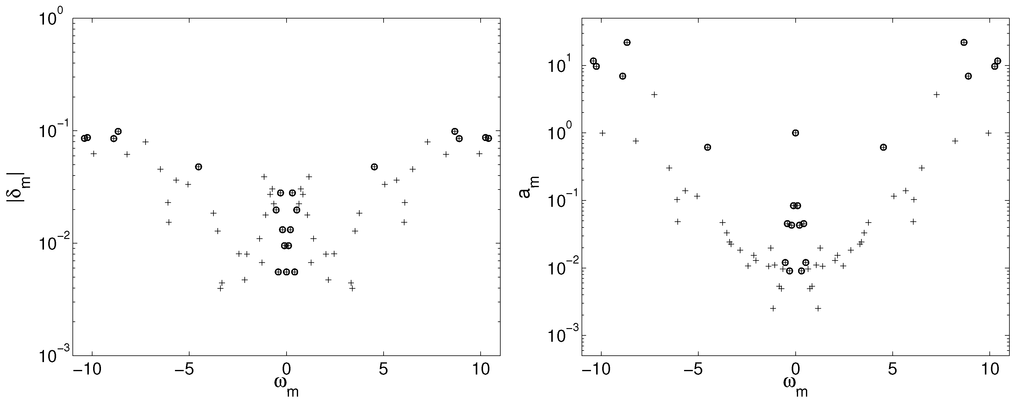
- The DMD-d approximation. The reduced snapshot matrix is used to construct the following matrix according to the higher order Koopman assumptionwhere the reduced Koopman operators contain the dynamics of the system. These are collected into a single matrix , called the modified Koopman matrix. The eigenvalues of the modified Koopman matrix represent the frequencies and growth/damping rates of equation (1), while the eigenvectors, combined with the SVD modes , are used to calculate the DMD modes (normalized to exhibit unit norm). Finally, the amplitudes related to each mode are calculated by least squares fitting of the expansion (1). In HODMD, the most relevant M DMD modes are retained as function of their amplitudes, depending on a second tolerance (set by the user), where
2.2.2. Criterion Selection Method
3. Numerical Results
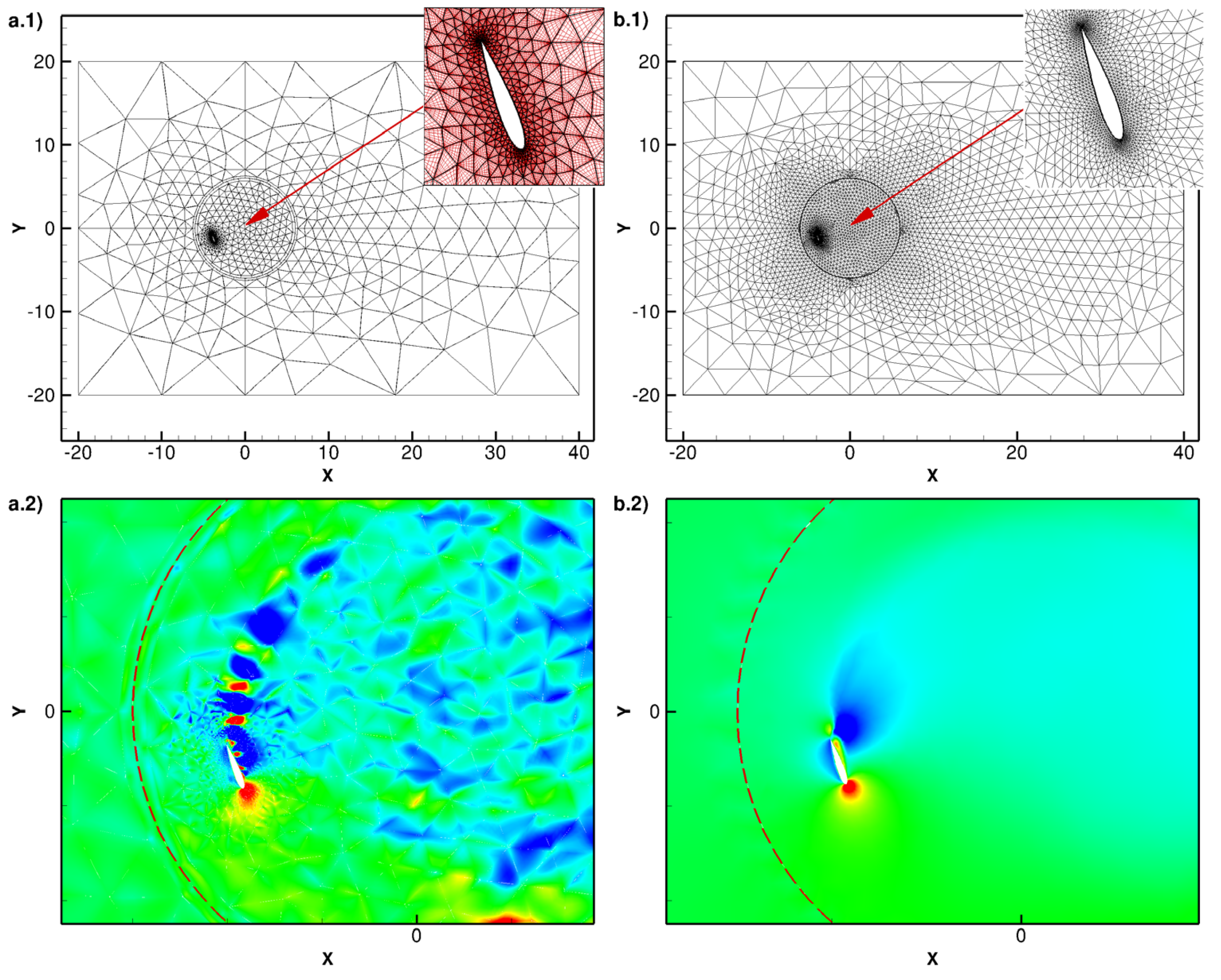
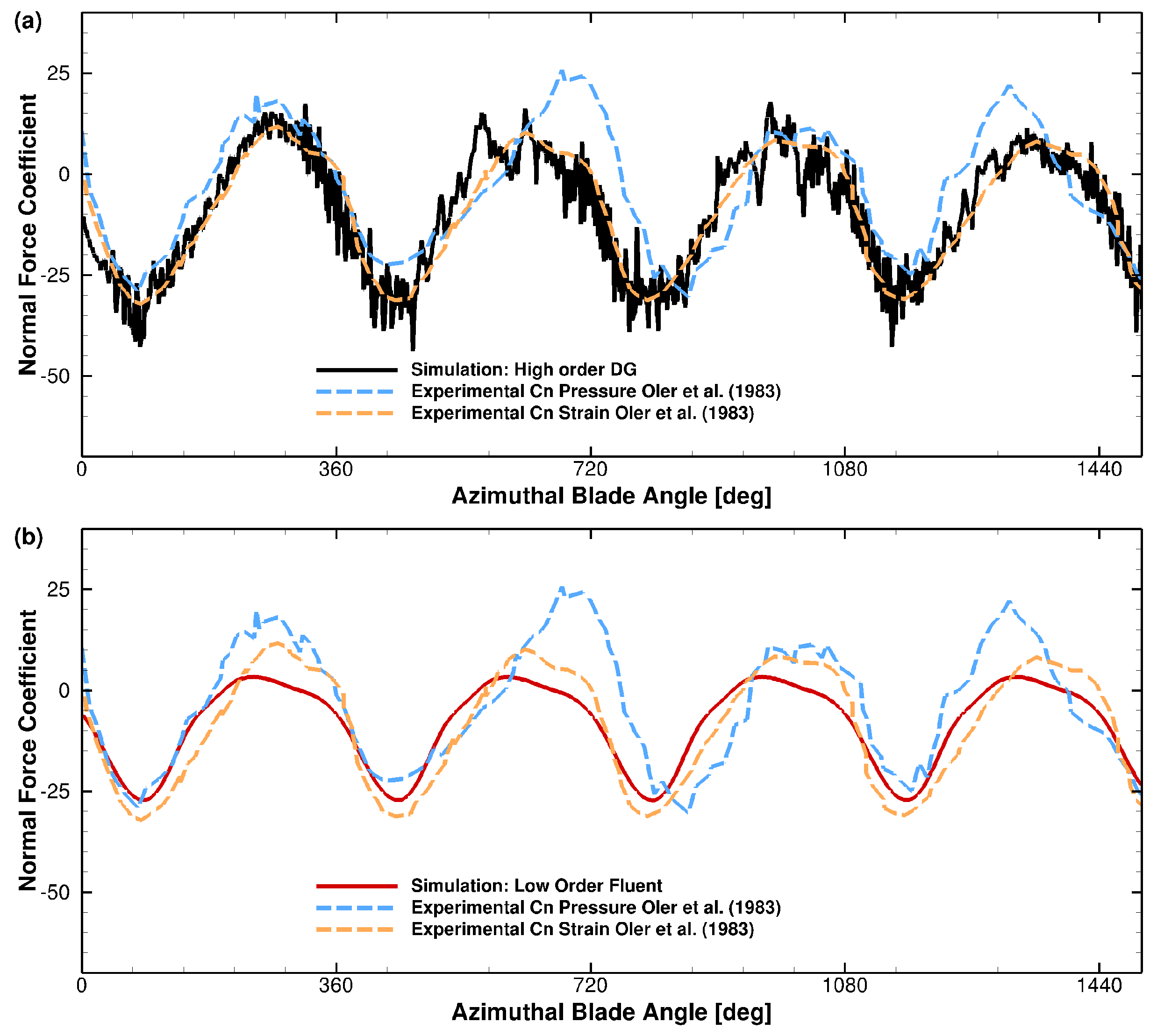
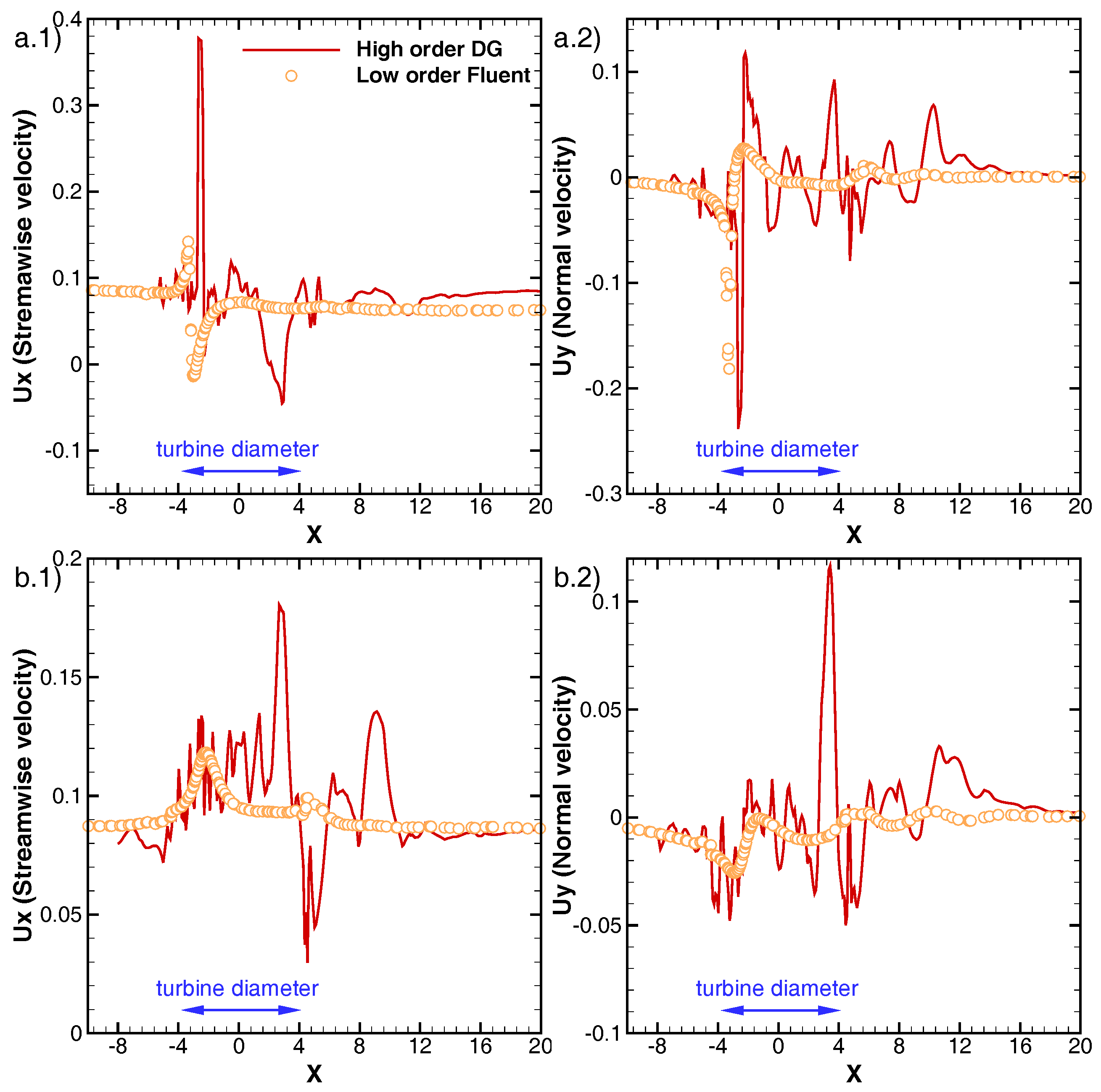
3.1. Numerical Simulations for a One Bladed Vertical Axis Turbines
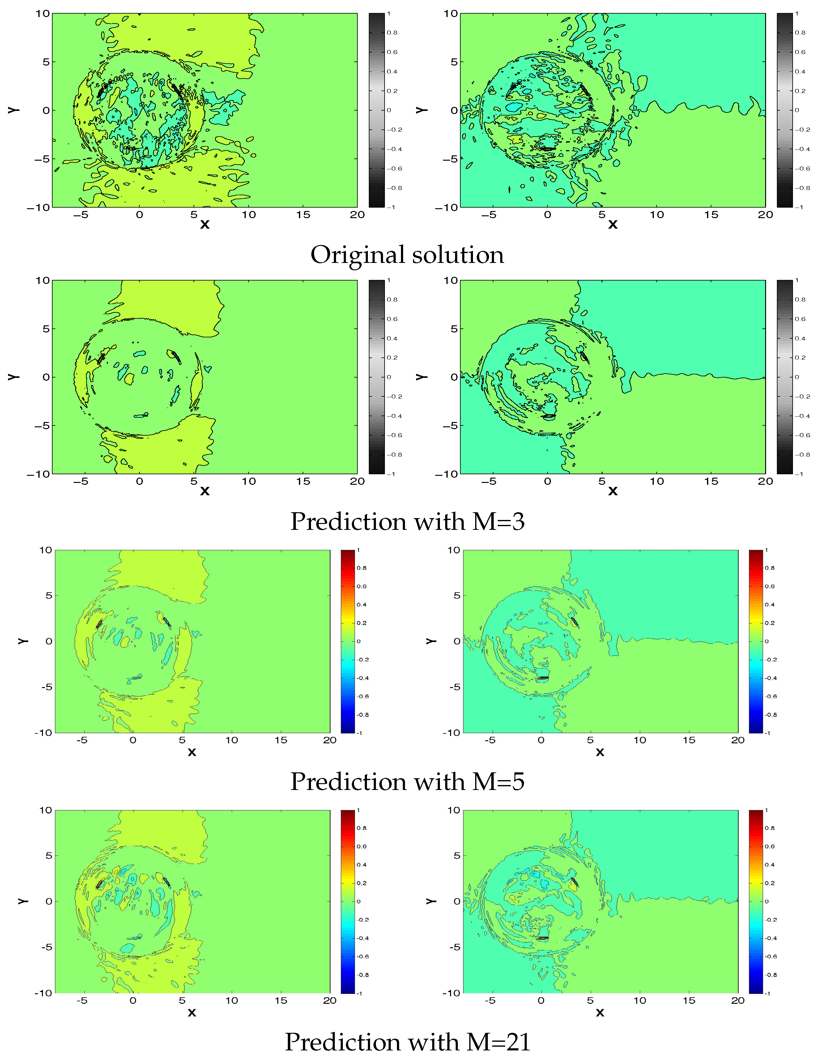
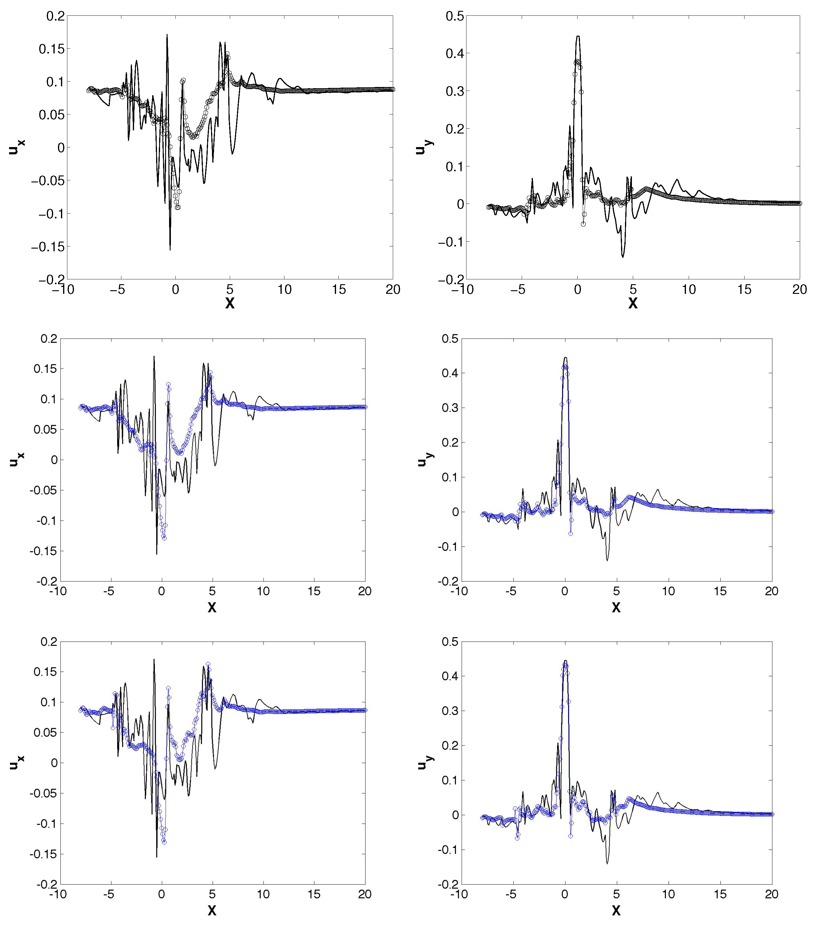
3.2. Reduced Order Model for a One Bladed Vertical Axis Turbine
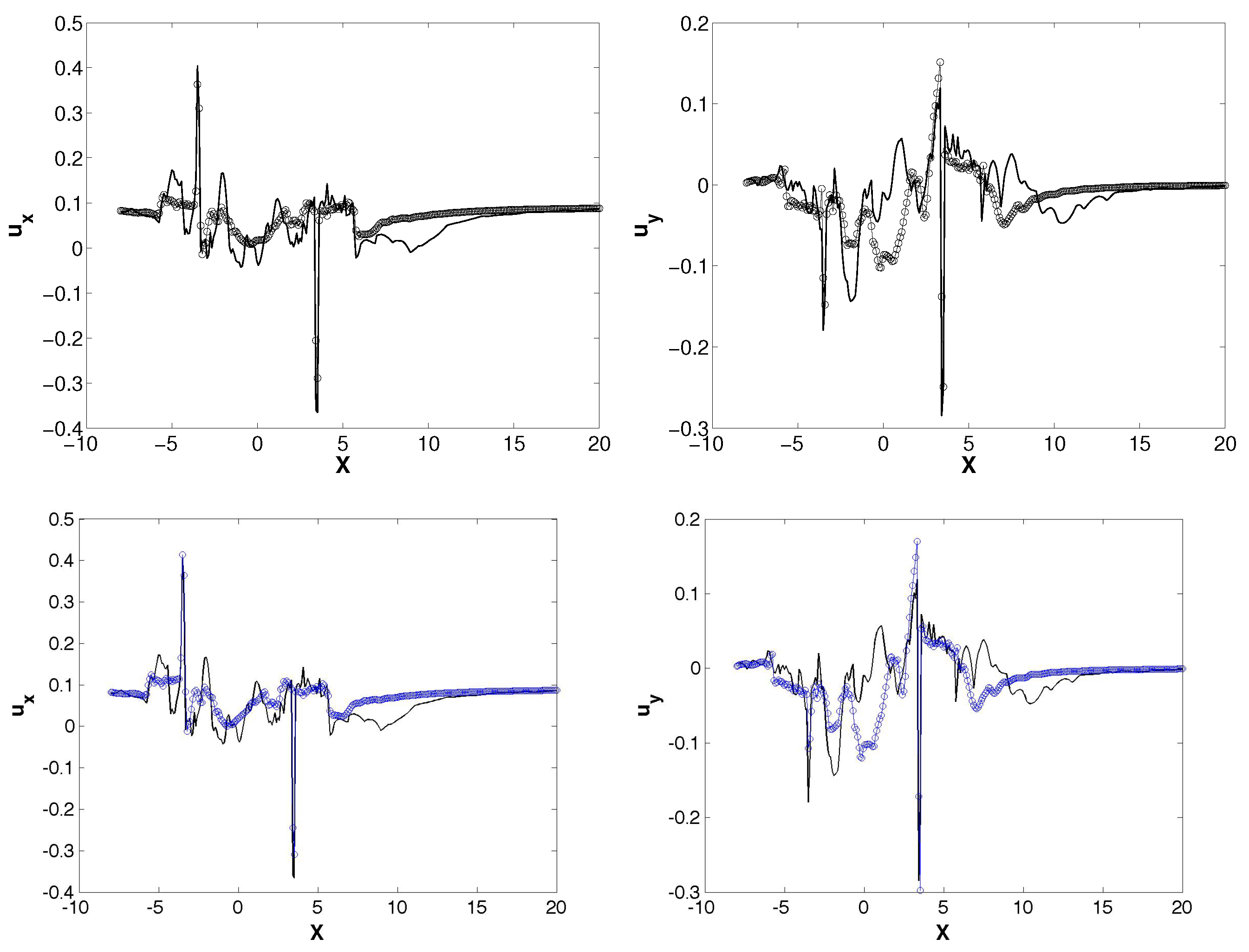
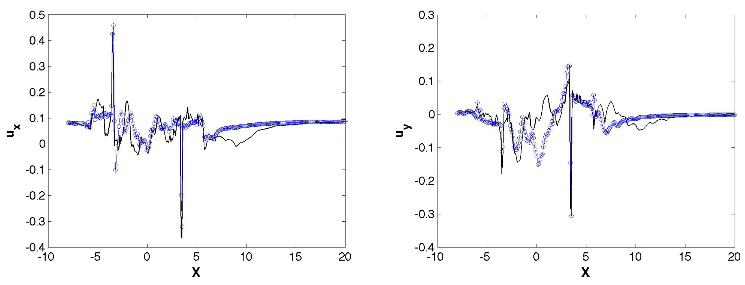
3.3. Extensions for Three Bladed Vertical Axis Turbine
4. Conclusions
Author Contributions
Conflicts of Interest
Abbreviations
| ROM | Reduced Order Model |
| DMD | Dynamic Mode Decomposition |
| HODMD | High Order Dynamic Mode Decomposition |
| DG | Discontinuous Galerkin |
| LES | Large Eddy Simulation |
| uRANS | unsteady Reynolds Averaged Navier–Stokes |
References
- Ferrer, E.; Willden, R.H.J. Blade-wake interactions in cross-flow turbines. Int. J. Mar. Energy 2015, 11, 71–83. [Google Scholar] [CrossRef]
- Eriksson, S.; Bernhoff, H.; Leijon, M. Evaluation of different turbine concepts for wind power. Renew. Sustain. Energy Rev. 2008, 12, 1419–1434. [Google Scholar] [CrossRef]
- Islam, M.; Ting, D.S.K.; Fartaj, A. Aerodynamic models for Darrieus-type straight-bladed vertical axis wind turbines. Renew. Sustain. Energy Rev. 2008, 12, 1087–1109. [Google Scholar] [CrossRef]
- Tjiu, W.; Marnoto, T.; Mat, S.; Ruslan, M.H.; Sopian, K. Darrieus vertical axis wind turbine for power generation I: Assessment of darrieus VAWT configurations. Renew. Energy 2015, 75, 50–67. [Google Scholar] [CrossRef]
- Muller, G.; Jentsch, M.F.; Stoddart, E. Vertical axis resistance type wind turbines for use in buildings. Renew. Energy 2009, 34, 1407–1412. [Google Scholar]
- Newman, B.G. Actuator-disc theory for vertical-axis wind turbines. J. Wind Eng. Ind. Aerodyn. 1983, 15, 347–355. [Google Scholar] [CrossRef]
- Sagaut, P. Large Eddy Simulation for Incompressible Flows: An Introduction; Scientific Computation; Springer: Berlin, Germany, 2001. [Google Scholar]
- Rowley, C.W.; Dawson, S.T.M. Model Reduction for Flow Analysis and Control. Annu. Rev. Fluid Mech. 2017, 49, 387–417. [Google Scholar] [CrossRef]
- Debnath, M.; Santoni, C.; Leonardi, S.; Iungo, G.V. Towards reduced order modelling for predicting the dynamics of coherent vorticity structures within wind turbine wakes. Philos. Trans. R. Soc. A Math. Phys. Eng. Sci. 2017, 375, 20160108. [Google Scholar] [CrossRef] [PubMed]
- Iungo, G.V.; Santoni-Ortiz, C.; Abkar, M.; Porte-Agel, F.; Rotea, M.A.; Leonardi, S. Data-driven Reduced Order Model for prediction of wind turbine wakes. J. Phys. Conf. Ser. 2015, 625, 012009. [Google Scholar] [CrossRef]
- Le Clainche, S.; Vega, J.M. Higher Order Dynamic Mode Decomposition. SIAM J. Appl. Dyn. Syst. 2017, 16, 882–925. [Google Scholar] [CrossRef]
- Kou, J.; Le Clainche, S.; Zhang, W. A reduced-order model for compressible flows with buffeting condition using higher order dynamic mode decomposition with a mode selection criterion. Phys. Fluids 2018, 30, 016103. [Google Scholar]
- Le Clainche, S.; Vega, J.M. Higher order dynamic mode decomposition to identify and extrapolate flow patterns. Phys. Fluids 2017, 29, 084102. [Google Scholar] [CrossRef]
- Wang, Z.J.; Fidkowski, R.; Abgrall, K.; Bassi, F.; Caraeni, D.; Cary, A.; Deconinck, H.; Hartmann, R.; Hillewaert, K.; Huynh, H.T.; et al. High-order CFD methods: Current status and perspective. Int. J. Numer. Methods Fluids 2013, 72, 811–845. [Google Scholar] [CrossRef]
- Ferrer, E.; Willden, R.H.J. A high order Discontinuous Galerkin Finite Element solver for the incompressible Navier-Stokes equations. Comput. Fluids 2011, 46, 224–230. [Google Scholar] [CrossRef]
- Ferrer, E.; Willden, R.H.J. A high order discontinuous Galerkin—Fourier incompressible 3D Navier-Stokes solver with rotating sliding meshes. J. Comput. Phys. 2012, 231, 7037–7056. [Google Scholar] [CrossRef]
- Ferrer, E. A high Order Discontinuous Galerkin—Fourier Incompressible 3D Navier-Stokes Solver with Rotating Sliding Meshes for Simulating Cross-Flow Turbines. Ph.D. Thesis, University of Oxford, Oxford, UK, 2012. [Google Scholar]
- Ferrer, E.; Moxey, D.; Willden, R.H.J.; Sherwin, S. Stability of projection methods for incompressible flows using high order pressure-velocity pairs of same degree: Continuous and discontinuous Galerkin formulations. Commun. Comput. Phys. 2014, 16, 817–840. [Google Scholar] [CrossRef]
- Ferrer, E. An interior penalty stabilised incompressible discontinuous Galerkin-Fourier solver for implicit Large Eddy Simulations. J. Comput. Phys. 2017, 348, 754–775. [Google Scholar] [CrossRef]
- Ferrer, E.; de Vicente, J.; Valero, E. Low cost 3d global instability analysis and flow sensitivity based on dynamic mode decomposition and high-order numerical tools. Int. J. Numer. Methods Fluids 2014, 76, 169–184. [Google Scholar] [CrossRef]
- González, L.; Ferrer, E.; Diaz-Ojeda, H.R. Onset of three dimensional flow instabilities in lid-driven circular cavities. Wind Eng. 2017, 29, 0641022. [Google Scholar] [CrossRef]
- Ferrer, E.; Le Clainche, S. Flow scales in cross-flow turbines. In CFD for Wind and Tidal Offshore Turbines; Springer International Publishing: Basel, Switzerland, 2015; pp. 1–11. [Google Scholar]
- Schmid, P.J. Dynamic mode decomposition of numerical and experimental data. J. Fluid Mech. 2010, 656, 5–28. [Google Scholar] [CrossRef]
- Le Clainche, S.; Vega, J.M.; Soria, J. Higher Order Dynamic Mode Decomposition for noisy experimental data: Flow structures on a Zero-Net-Mass-Flux jet. Exp. Therm. Fluid Sci. 2017, 88, 336–353. [Google Scholar] [CrossRef]
- Le Clainche, S.; Moreno-Ramos, R.; Taylor, P.; Vega, J.M. A new robust method to study flight flutter testing. J. Aircr. Submitted.
- Berkooz, G.; Holmes, P.; Lumley, J. The proper orthogonal decomposition in the analysis of turbulent flows. Annu. Rev. Fluid Mech. 1993, 25, 539–575. [Google Scholar] [CrossRef]
- Kou, J.; Zhang, W. An improved criterion to select dominant modes of dynamic mode decomposition. Eur. J. Mech. B Fluids 2017, 62, 109–129. [Google Scholar] [CrossRef]
- Sirovich, L. Turbulence and the dynamic of coherent structures, parts I–III. Q. Appl. Math. 1987, 45, 561–571. [Google Scholar] [CrossRef]
- Le Clainche, S.; Sastre, F.; Vega, J.M.; Velázquez, A. Higher order dynamic mode decomposition applied to postproces a limited amount of PIV data. In Proceedings of the 47th AIAA Fluid Dynamics Conference, AIAA Aviation Forum (AIAA paper 2017-3304), Denver, CO, USA, 5–9 June 2017. [Google Scholar]
- Le Clainche, S.; Pérez, J.M.; Vega, J.M. Spatio-temporal flow structures in the three-dimensional wake of a circular cylinder. Fluid Dyn. Res. 2018. [Google Scholar] [CrossRef]
- Sayadi, T.; Schmid, P.J.; Richecoeur, F.; Durox, D. Parametrized datadriven decomposition for bifurcation analysis, with application to thermoacoustically unstable systems. Phys. Fluids 2015, 27, 037102. [Google Scholar] [CrossRef]
- Bazilevs, Y.; Korobenko, A.; Deng, X.; Yan, J.; Kinzel, M.; Dabiri, J.O. Fluid-structure interaction modeling of vertical-axis wind turbines. J. Appl. Mech. 2014, 81, 081006. [Google Scholar] [CrossRef]
- Consul, C.A.; Willden, R.H.; McIntosh, S.C. Blockage effects on the hydrodynamic performance of a marine cross-flow turbine. Philos. Trans. R. Soc. A Math. Phys. Eng. Sci. 2013, 371, 20120299. [Google Scholar] [CrossRef] [PubMed]
- Howell, R.; Qin, N.; Edwards, J.; Durrani, N. Wind tunnel and numerical study of a small vertical axis wind turbine. Wind Eng. 2010, 35, 412–422. [Google Scholar] [CrossRef]
- Hsu, M.C.; Akkerman, I.; Bazilevs, Y. High-performance computing of wind turbine aerodynamics using isogeometric analysis. Comput. Fluids 2011, 49, 93–100. [Google Scholar] [CrossRef]
- McLaren, K.; Tullis, S.; Ziada, S. Computational fluid dynamics simulation of the aerodynamics of a high solidity, small-scale vertical axis wind turbine. Wind Energy 2011, 15, 349–361. [Google Scholar] [CrossRef]
- Qin, N.; Howell, R.; Durrani, N.; Hamada, K.; Smith, T. Unsteady flow simulation and dynamic stall behaviour of vertical axis wind turbine blades. Wind Eng. 2011, 35, 511–527. [Google Scholar] [CrossRef]
- Fluent Manual—ANSYS Academic Research, Release 16.2; ANSYS, Inc.: Canonsburg, PA, USA, 2015.
- Oler, J.W.; Strickland, J.H.; Im, B.J.; Graham, G.H. Dynamic Stall Regulation of Thedarrieus Turbine; Technical Report, SANDIA REPORT SAND83-7029 UC-261; Sandia National Laboratories: Albuquerque, NM, USA, 1983. [Google Scholar]
- Bremseth, J.; Duraisamy, K. Computational analysis of vertical axis wind turbine arrays. Theor. Comput. Fluid Dyn. 2016, 30, 387–401. [Google Scholar] [CrossRef]
- Chen, Y.; Lian, Y. Numerical investigation of vortex dynamics in an H-rotor vertical axis wind turbine. Eng. Appl. Comput. Fluid Mech. 2015, 1, 21–32. [Google Scholar] [CrossRef]
- Deglaire, P.; Engblom, S.; Ågren, O.; Bernhoff, H. Analytical solutions for a single blade in vertical axis turbine motion in two-dimensions. Eur. J. Mech. B Fluids 2009, 28, 506–520. [Google Scholar] [CrossRef]
- Osterberg, D. Multi-Body Unsteady Aerodynamics in 2D Applied to a Vertical-Axis Wind Turbine Using a Vortex Method; Technical Report; Uppsala University: Uppsala, Sweden, 2010. [Google Scholar]


| High Order Solver | Low Order Fluent | |
|---|---|---|
| Blade/Mesh movement | Sliding mesh | Sliding mesh |
| Numerical scheme | 3D DG-Fourier | 2D Finite Volume |
| Out-of-plane length | 0.5 m * | 0 m |
| Turbulence model | Large Eddy Simulation | k-omega SST (uRANS) |
| Numerical details | polynomial order P = 3 | Second order Upwind |
| Order of accuracy | 3 | 2 |
| Mesh size | 1.1 millions ** | 7896 *** |
| Time advancement | 2nd order semi-implicit | 1st order implicit |
| Time step | 0.001 s | 0.2 s |
| Blade | Turb. | Length | Stream | Rot. | Tip Speed | Kin. | Reynolds | ||
|---|---|---|---|---|---|---|---|---|---|
| Chord | Diameter | Ratio | Vel. | Speed | Ratio | Visc | |||
| Symbol | c | D | U | ||||||
| Units | m | m | - | m/s | rad/s | - | m2/s | - | - |
| Oler et al. [39] | 0.1524 | 1.22 | 0.125 | 0.091 | 0.749 | 5 | |||
| Simulations | 1.0 | 8.0 | 0.125 | 0.088 | 0.11 | 5 | |||
| m | M | |||
|---|---|---|---|---|
| 1 | −9.5158 × | 1.0418 × | 8.3676 × | 3 |
| 2 | −1.3190 × | 2.0196 × | 4.3080 × | 5 |
| 3 | −5.5556 × | 4.2243 × | 4.5354 × | 7 |
| 4 | 8.5601 × | 1.0403 × 10 | 1.1669 × 10 | 9 |
| 5 | 9.8704 × | 8.6673 | 2.1948 × 10 | 11 |
| 6 | 8.7053 × | 1.0250 × 10 | 9.6744 | 13 |
| 7 | −2.8024 × | 3.0565 × | 9.0310 × | 15 |
| 8 | 4.7800 × | 4.5260 | 6.1397 × | 17 |
| 9 | −1.9750 × | 5.2824 × | 1.2018 × | 19 |
| 10 | 8.5236 × | 8.8956 | 6.9477 | 21 |
| m | M | |||
|---|---|---|---|---|
| 1 | −2.4974 × | 1.0372 × | 1.4785 × | 3 |
| 2 | −5.6401 × | 2.1195 × | 9.5278 × | 5 |
| 3 | −2.6524 × | 3.3103 × | 2.9438 × | 7 |
| 4 | −2.9580 × | 4.3577 × | 2.2503 × | 9 |
| 5 | −3.2188 × | 5.4754 × | 1.8342 × | 11 |
| 6 | −2.8720 × | 6.5329 × | 1.7896 × | 13 |
| 7 | −2.7517 × | 7.8174 × | 1.3842 × | 15 |
| 8 | −2.8857 × | 1.0277 | 1.2363 × | 17 |
| 9 | −4.0700 × | 1.1119 | 1.1227 × | 19 |
| 10 | −4.2714 × | 1.2517 | 8.6121 × | 21 |
| m | M | |||
|---|---|---|---|---|
| 1 | −3.0199 × | 1.3516 × | 8.5508 × | 3 |
| 2 | −4.0940 × | 2.6042 × | 4.9633 × | 5 |
| 3 | −3.0227 × | 4.2156 × | 4.3403 × | 7 |
| 4 | −4.0559 × | 5.9441 × | 3.7762 × | 9 |
| 5 | −5.0647 × | 8.5848 × | 3.0700 × | 11 |
| 6 | −9.1483 × | 1.4785 | 2.2538 × | 13 |
| 7 | −3.8967 × | 1.1690 | 3.1258 × | 15 |
| 8 | −1.0826 × | 1.5864 | 1.8197 × | 17 |
| 9 | −6.2864 × | 1.3355 | 2.3832 × | 19 |
| 10 | −7.8737 × | 7.2259 × | 2.0244 × | 21 |
© 2018 by the authors. Licensee MDPI, Basel, Switzerland. This article is an open access article distributed under the terms and conditions of the Creative Commons Attribution (CC BY) license (http://creativecommons.org/licenses/by/4.0/).
Share and Cite
Le Clainche, S.; Ferrer, E. A Reduced Order Model to Predict Transient Flows around Straight Bladed Vertical Axis Wind Turbines. Energies 2018, 11, 566. https://doi.org/10.3390/en11030566
Le Clainche S, Ferrer E. A Reduced Order Model to Predict Transient Flows around Straight Bladed Vertical Axis Wind Turbines. Energies. 2018; 11(3):566. https://doi.org/10.3390/en11030566
Chicago/Turabian StyleLe Clainche, Soledad, and Esteban Ferrer. 2018. "A Reduced Order Model to Predict Transient Flows around Straight Bladed Vertical Axis Wind Turbines" Energies 11, no. 3: 566. https://doi.org/10.3390/en11030566
APA StyleLe Clainche, S., & Ferrer, E. (2018). A Reduced Order Model to Predict Transient Flows around Straight Bladed Vertical Axis Wind Turbines. Energies, 11(3), 566. https://doi.org/10.3390/en11030566