Spatiotemporal Patterns of Carbon Emissions and Taxi Travel Using GPS Data in Beijing


Abstract
:1. Introduction
2. Methodology
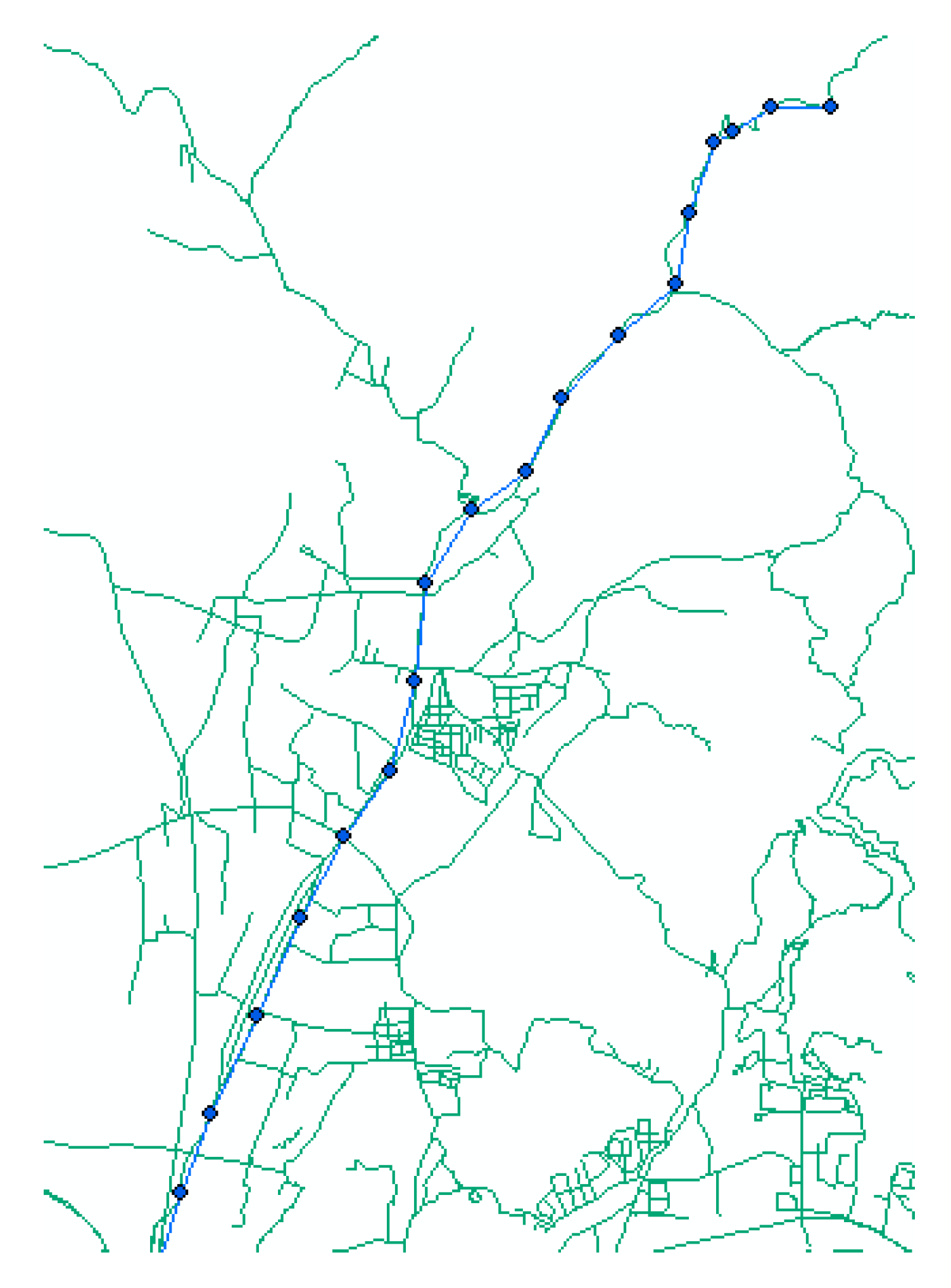
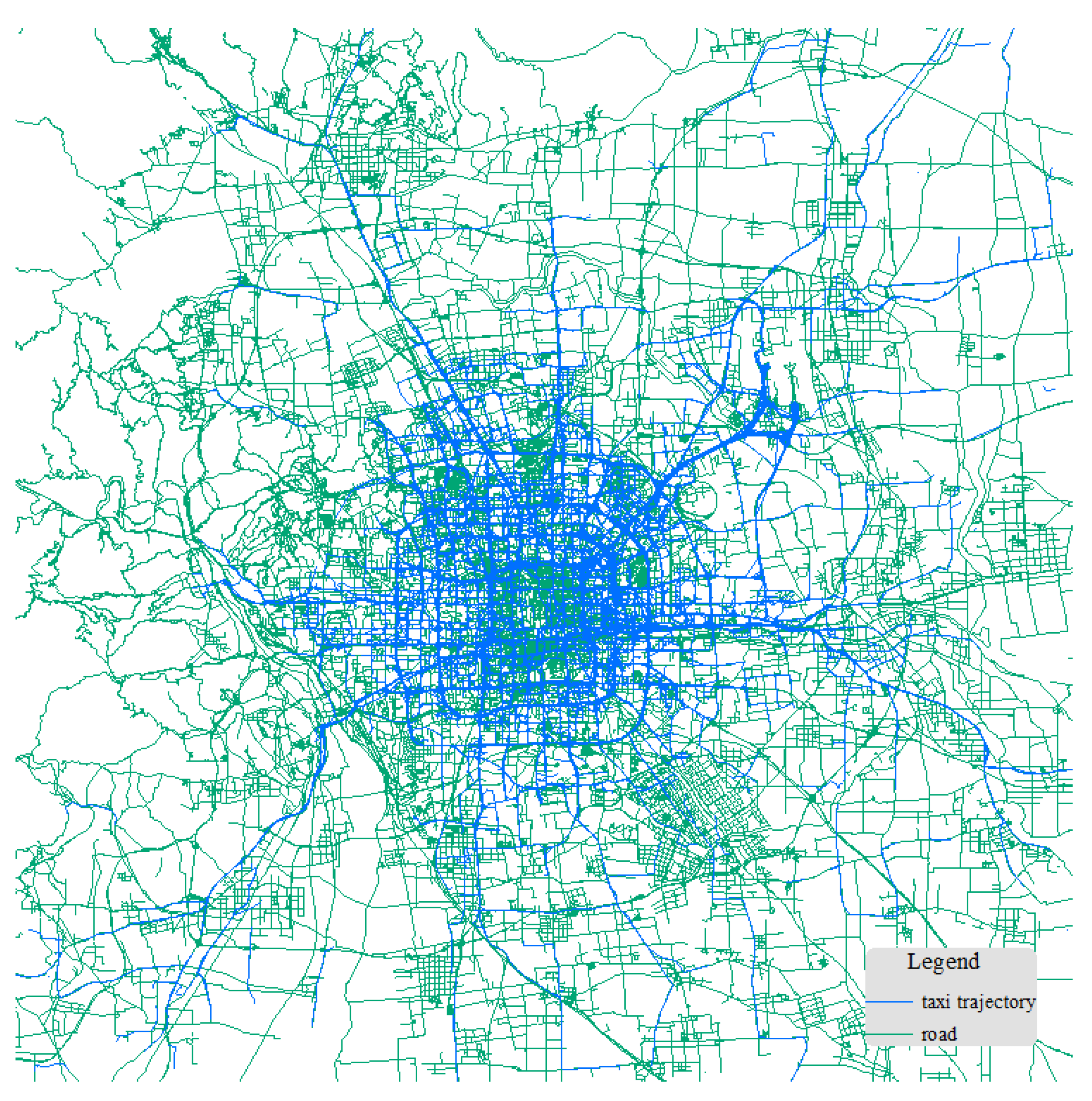
2.1. Description and Data Cleaning of Taxi GPS Data
2.2. Carbon Emission Calculation Model
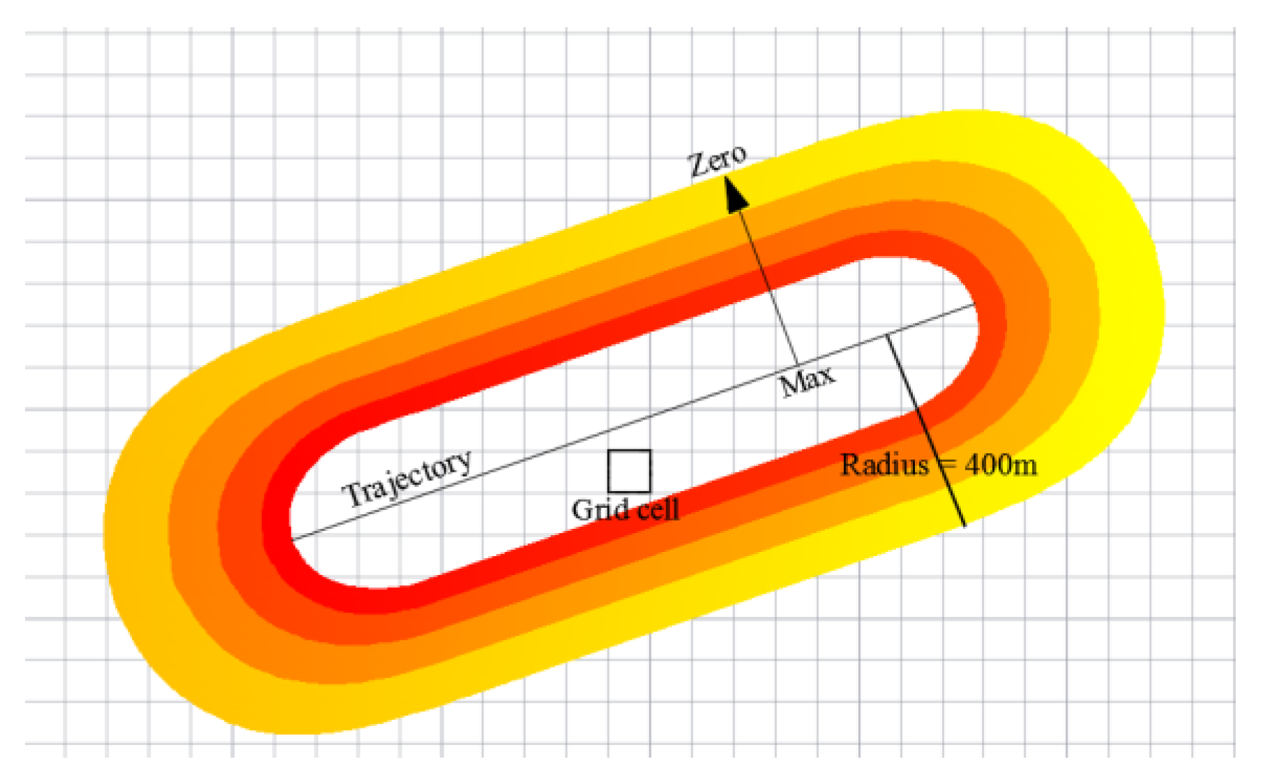
2.3. Taxi Carbon Emission Visualization Method
3. Case Study
4. Discussion
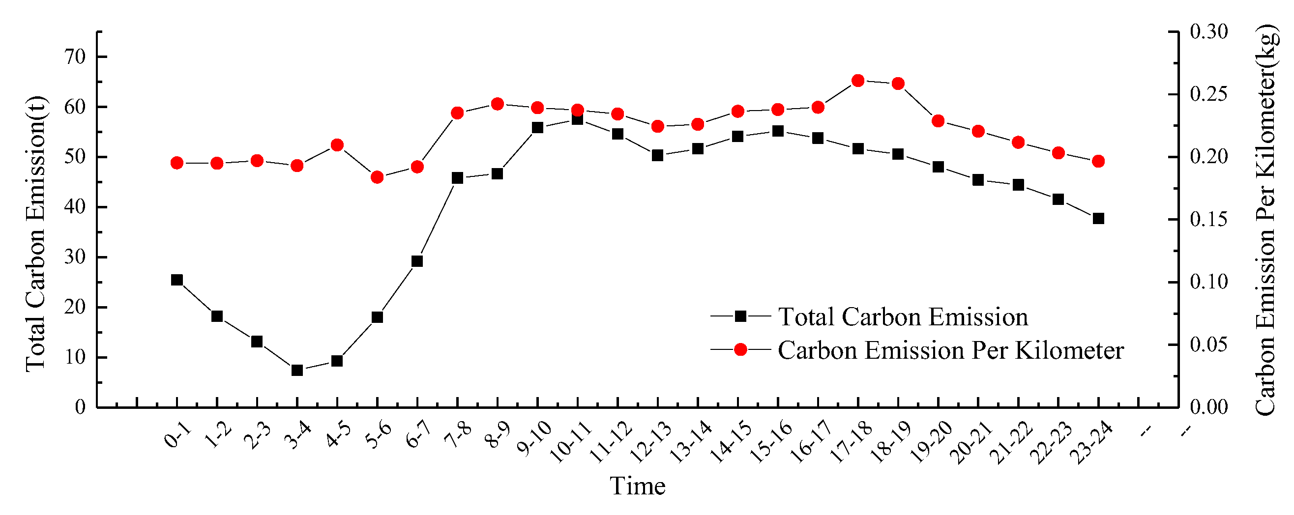
4.1. Temporal Carbon Emissions and Taxi Travel Patterns
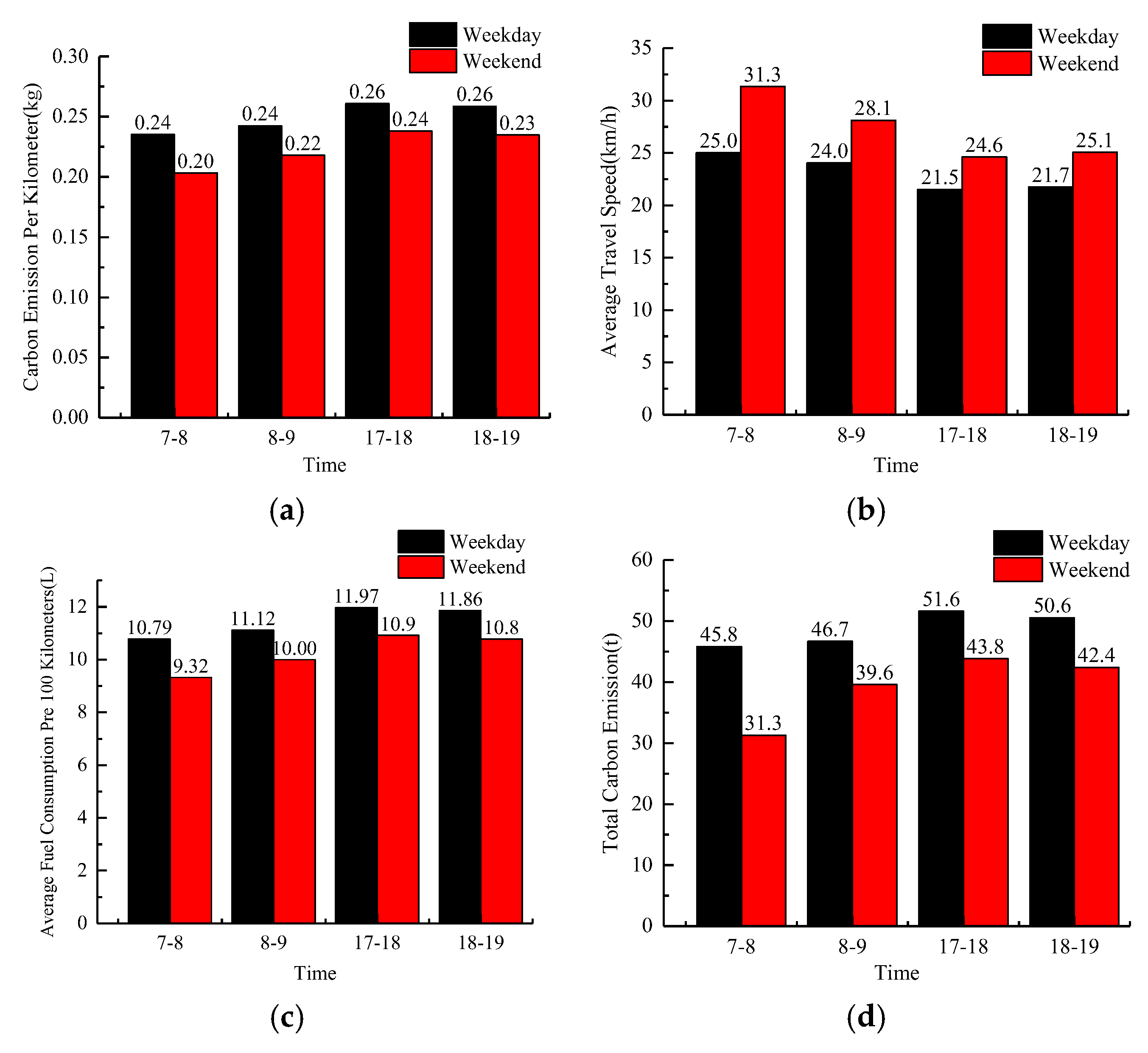
4.2. Temporal Comparison of Carbon Emissions and Travel Patterns between Weekdays and Weekends
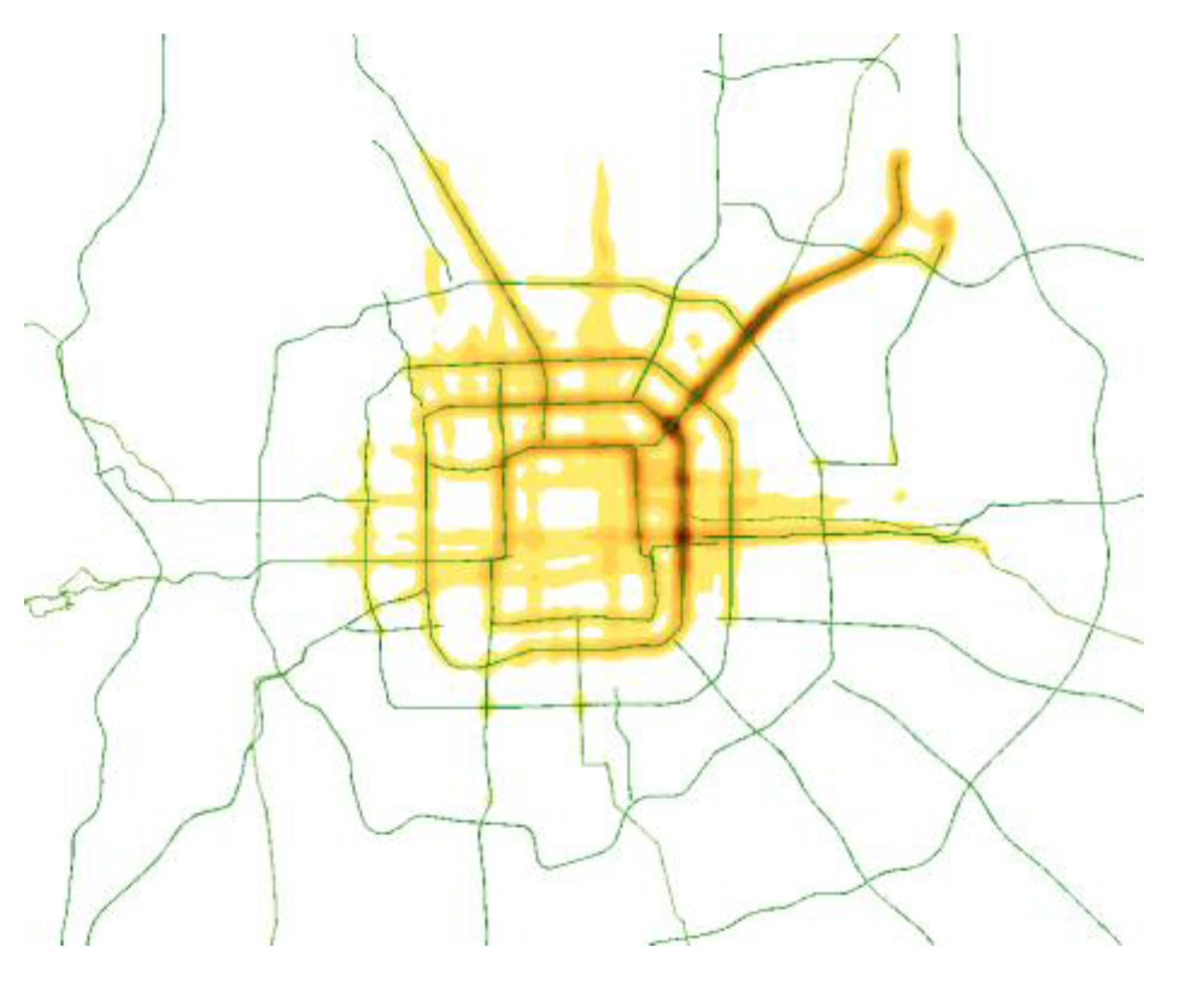
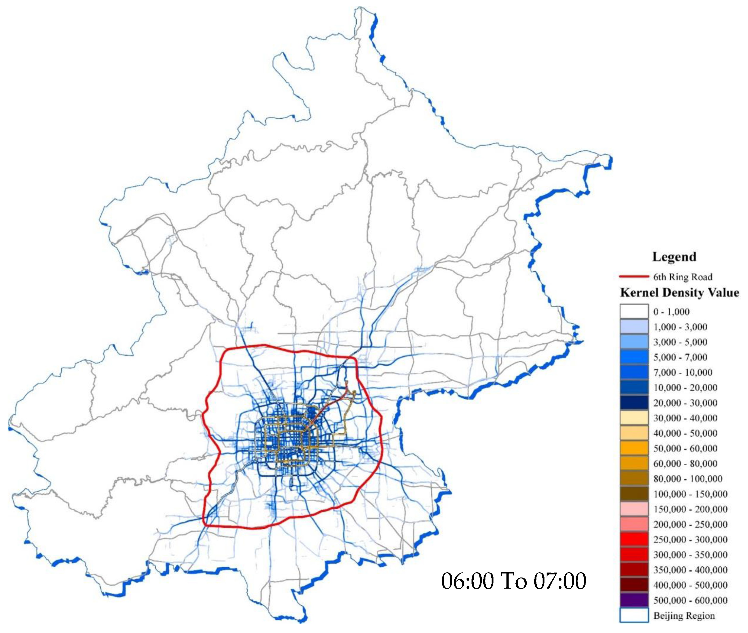
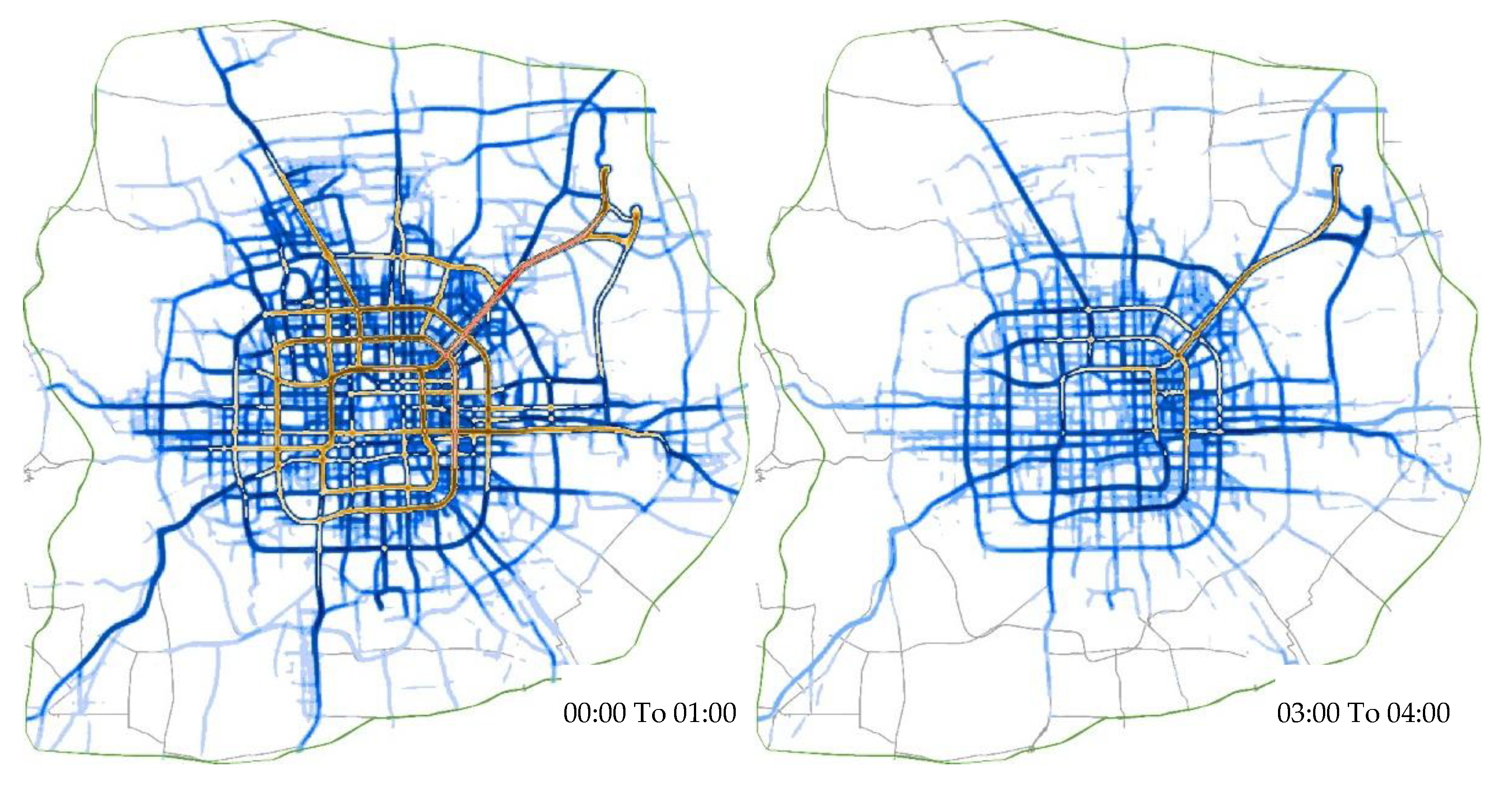
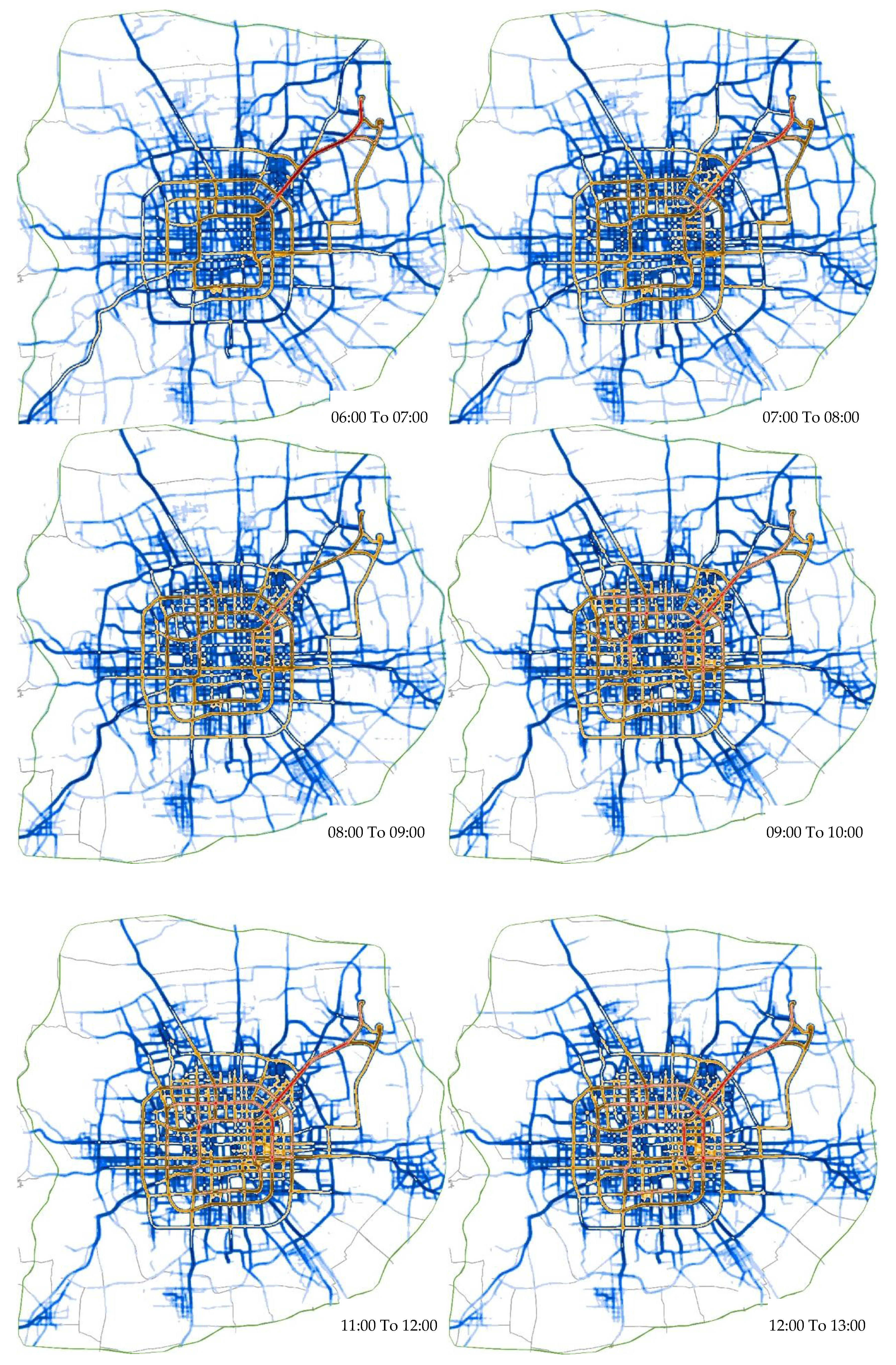
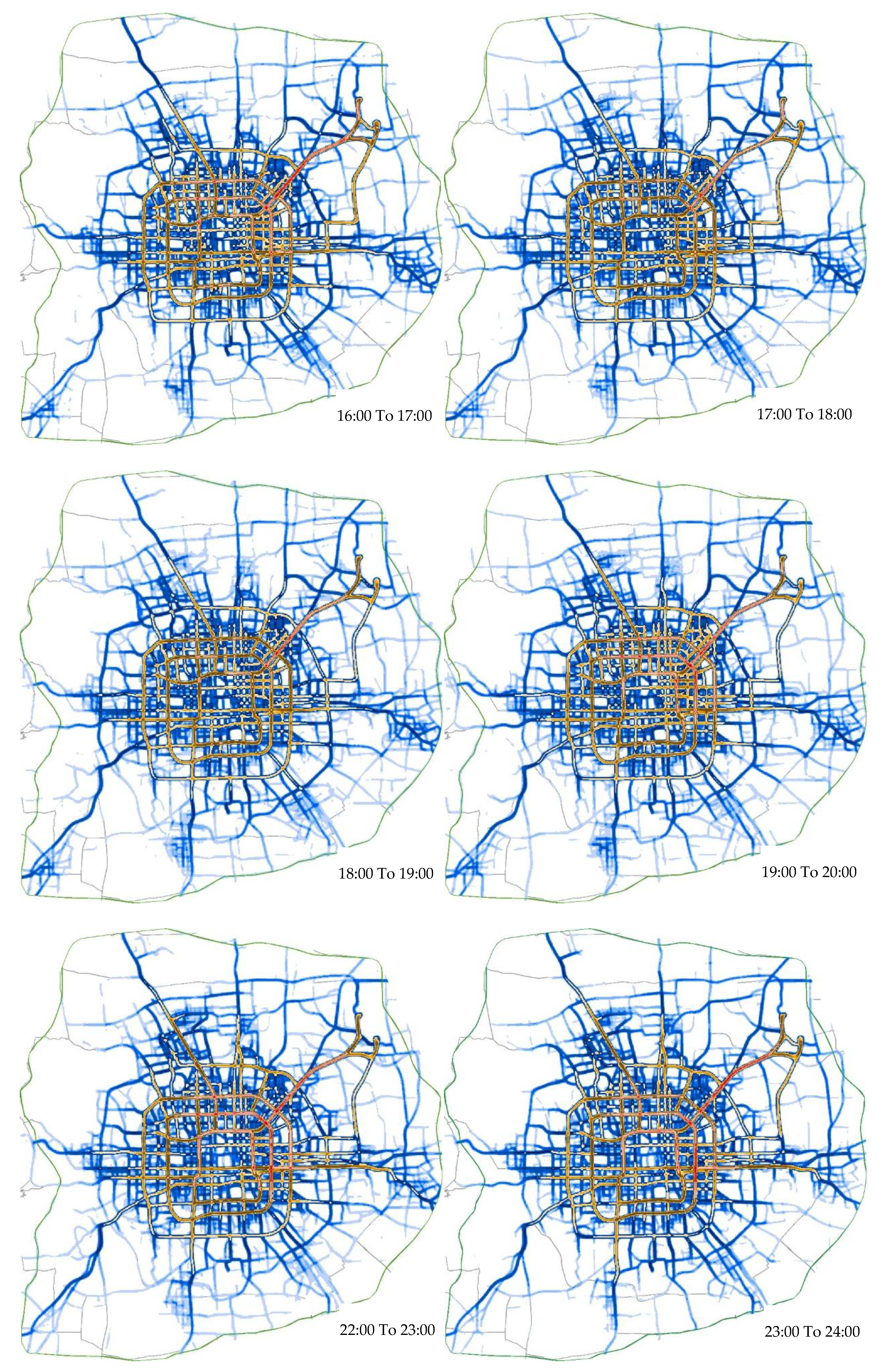
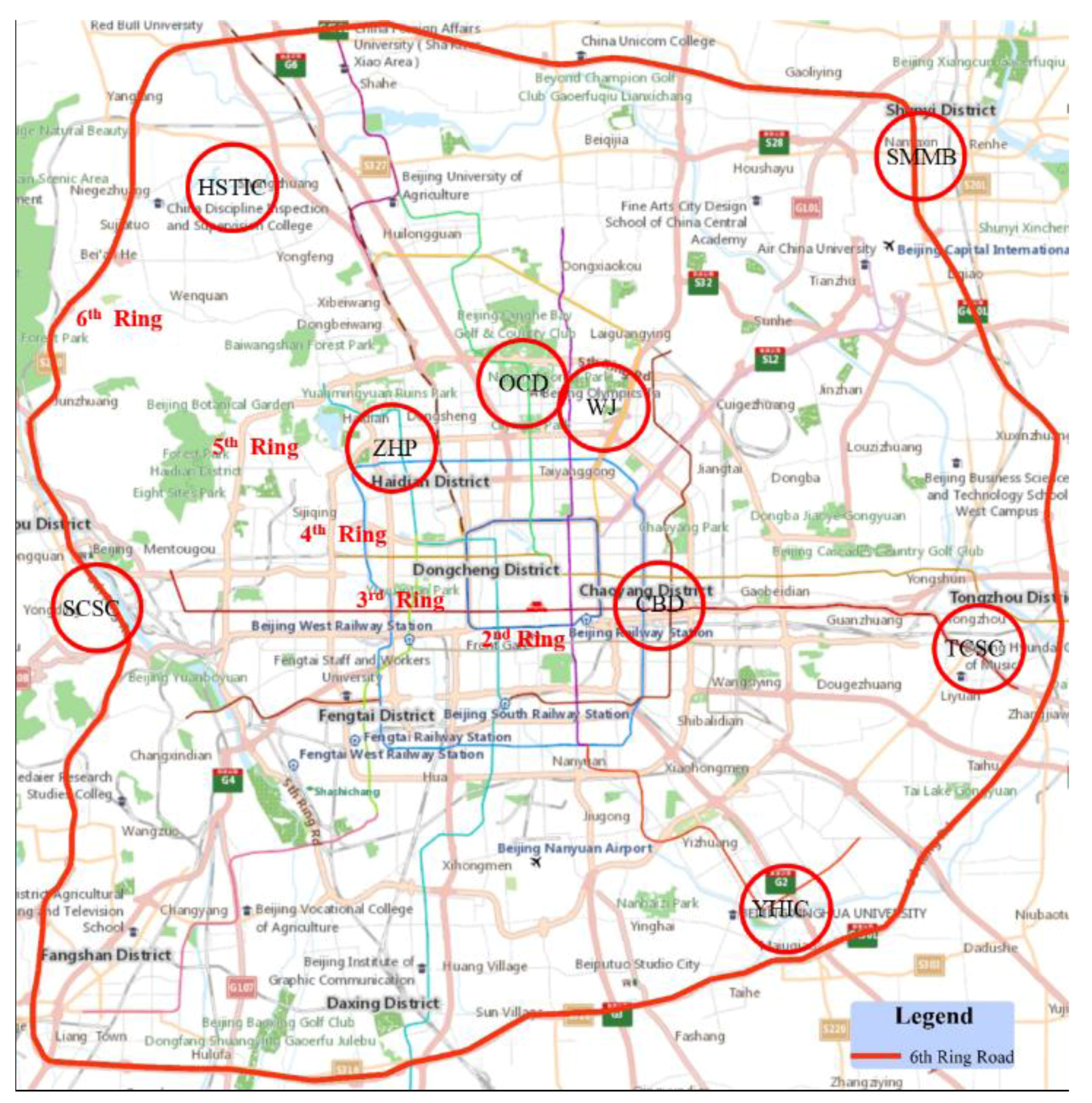
4.3. Spatial Carbon Emission Patterns
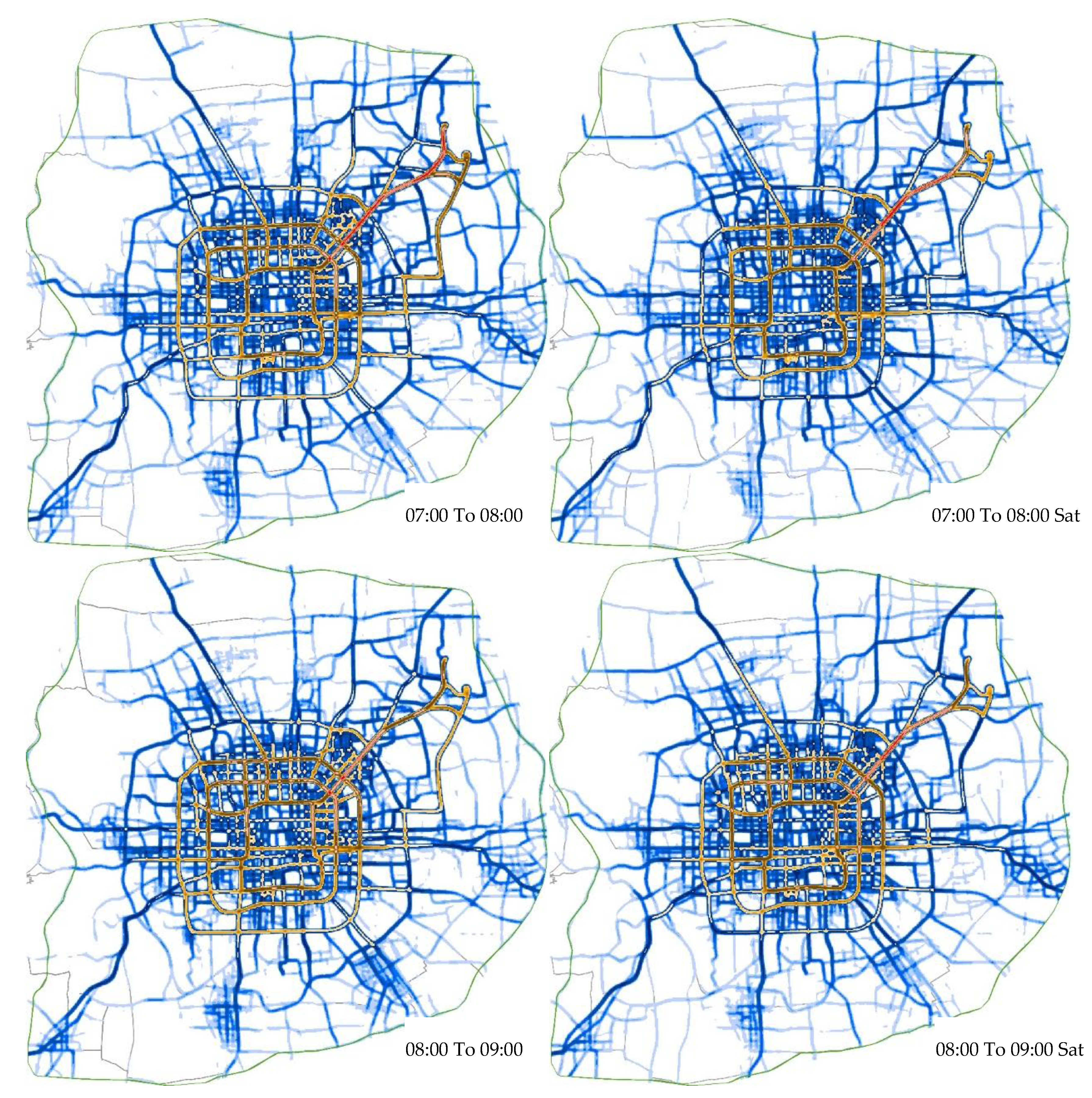
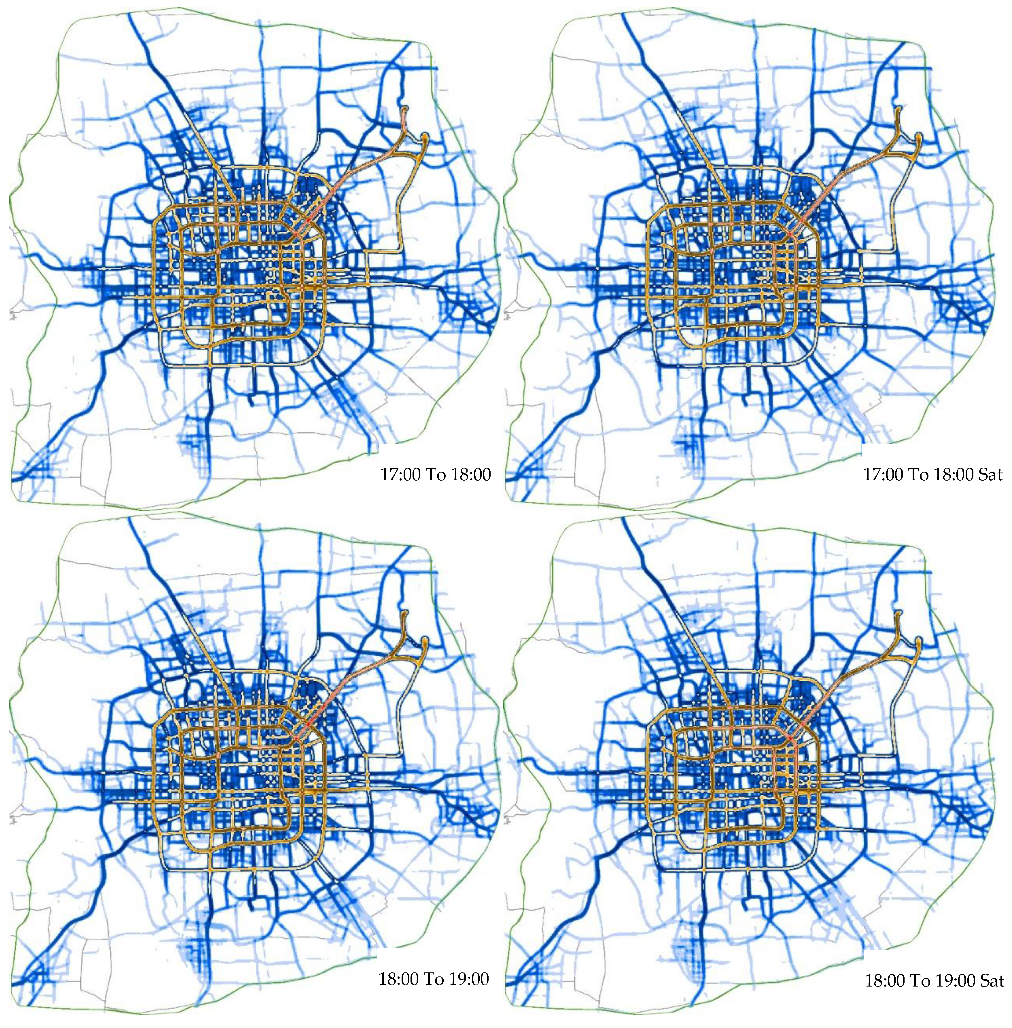
4.4. Spatial Comparison of Carbon Emissions between Weekdays and Weekends
5. Conclusions
- (1)
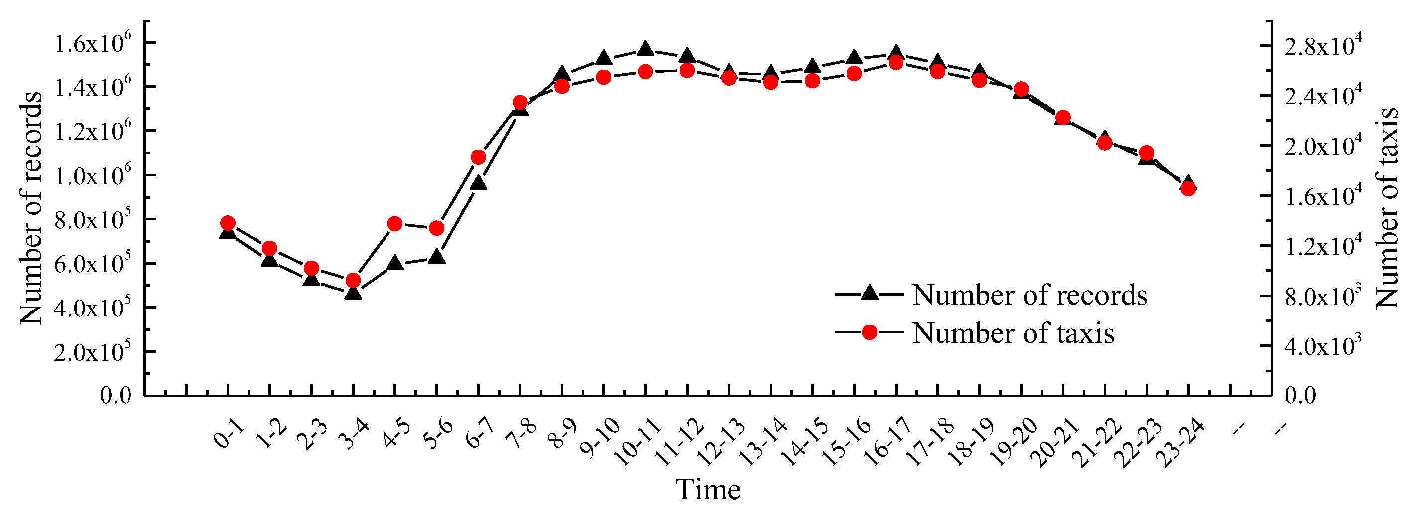
- The network-scale travel patterns of taxi fleets are clearly observed from taxi numbers.
- (2)
- The level of carbon emissions over the whole network can be evaluated via CEPK and total carbon emissions.
- (3)
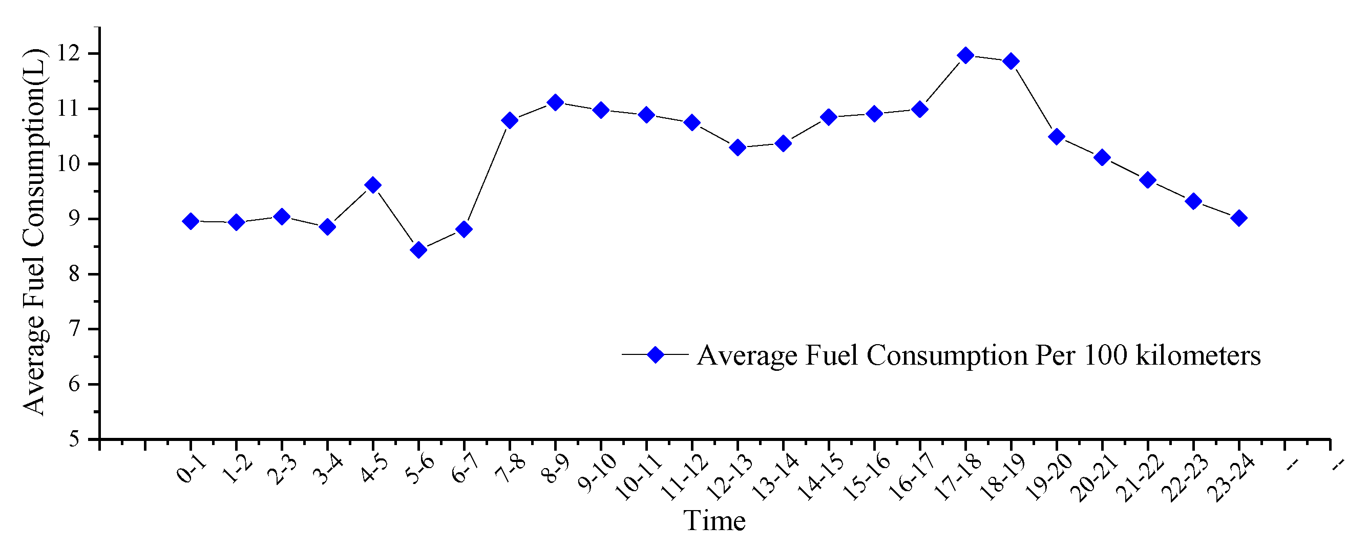
- Although the average FCPOK we obtained from taxi GPS data is higher than expected, it can allow policy makers to issue stricter regulations on carbon emission reduction.
- (4)
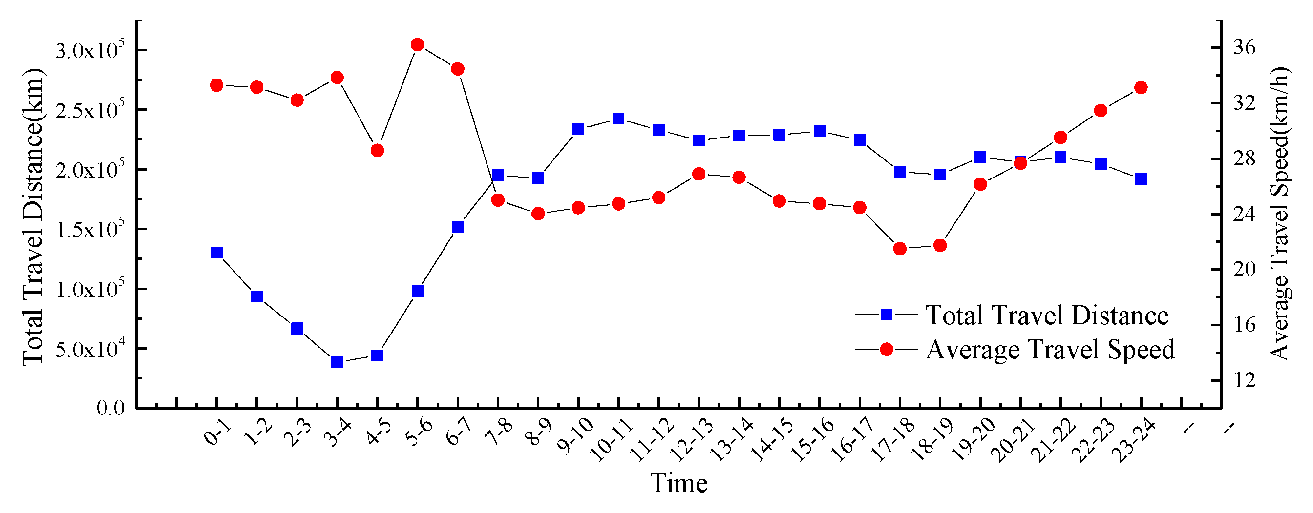
- The average travel speed by hour can be used to monitor traffic conditions over an entire urban network. The results indicate that higher resolution travel speed data, such as the average travel speed in one minute, can be obtained to instantly monitor traffic conditions, providing that it is feasible for the hardware. The average travel speed of the entire day over the whole network is lower than the official figure, which means that the traffic situation is more serious than previously thought.
- (5)
- Overall, carbon emissions and travel patterns show improvements on the weekend, especially during the morning rush hour period, because most people do not commute on the weekend.
- (6)
- By employing the visualization method, we creatively present the spatial dynamic distribution of carbon emissions with time. Using this method, authorities can instantaneously monitor the distribution of carbon emissions.
Supplementary Materials
Acknowledgments
Author Contributions
Conflicts of Interest
References
- Yang, L.; Kwan, M.; Pan, X.; Wan, B.; Zhou, S. Scalable space-time trajectory cube for path-finding: A study using big taxi trajectory data. Transp. Res. Part B Methodol. 2017, 101, 1–27. [Google Scholar] [CrossRef]
- Zhang, J.; Meng, W.; Liu, Q.Q.; Jiang, H.; Feng, Y.; Wang, G. Efficient vehicles path planning algorithm based on taxi GPS big data. Opt. Int. J. Light Electron Opt. 2016, 127, 2579–2585. [Google Scholar] [CrossRef]
- Lin, N. Path Planning Method Based on Taxi Trajectory Data. J. Inf. Comput. Sci. 2015, 12, 3395–3403. [Google Scholar] [CrossRef]
- Hu, J.; Huang, Z.; Deng, J.; Xie, H. Hierarchical Path Planning Method Based on Taxi Driver Experiences. J. Transp. Syst. Eng. Inf. Technol. 2013, 13, 185–192. [Google Scholar]
- Li, Q.; Zeng, Z.; Zhang, T.; Li, J.; Wu, Z. Path-finding through flexible hierarchical road networks: An experiential approach using taxi trajectory data. Int. J. Appl. Earth Obs. Geoinf. 2011, 13, 110–119. [Google Scholar] [CrossRef]
- Yuan, J.; Zheng, Y.; Zhang, C.; Xie, W.; Xie, X.; Sun, G.; Huang, Y. T-drive: Driving directions based on taxi trajectories. In Proceedings of the 18th SIGSPATIAL International Conference on Advances in Geographic Information Systems, San Jose, CA, USA, 2–5 November 2010; pp. 99–108. [Google Scholar]
- Meng, L.; Li, R.T.; Yong, X.; Qin, Z.G. Analysis of Urban Traffic Based on Taxi GPS Data. Lect. Notes Electr. Eng. 2014, 279, 1007–1015. [Google Scholar]
- Shan, Z.; Wang, Y.; Zhu, Q. Feasibility study of urban road traffic state estimation based on taxi GPS data. In Proceedings of the 17th IEEE International Conference on Intelligent Transportation Systems, Qingdao, China, 8–11 October 2014; pp. 2188–2193. [Google Scholar]
- Zhang, K.; Sun, D.; Shen, S.; Zhu, Y. Analyzing spatiotemporal congestion pattern on urban roads based on taxi GPS data. J. Transp. Land Use 2017, 10, 675–694. [Google Scholar] [CrossRef]
- Kong, X.; Yang, J.; Yang, Z. Measuring Traffic Congestion with Taxi GPS Data and Travel Time Index. In Proceedings of the 15th COTA International Conference of Transportation Professionals, Beijing, China, 24–27 July 2015. [Google Scholar]
- Kuang, W.; An, S.; Jiang, H. Detecting Traffic Anomalies in Urban Areas Using Taxi GPS Data. Math. Probl. Eng. 2015, 2015, 809582. [Google Scholar] [CrossRef]
- Chen, C.; Zhang, D.; Castro, P.S.; Li, N.; Sun, L.; Li, S. Real-Time Detection of Anomalous Taxi Trajectories from GPS Traces. In Mobile and Ubiquitous Systems: Computing, Networking, and Services; Springer: Berlin/Heidelberg, Germany, 2012. [Google Scholar]
- Pang, L.X.; Chawla, S.; Liu, W.; Zheng, Y. On detection of emerging anomalous traffic patterns using GPS data. Data Knowl. Eng. 2013, 87, 357–373. [Google Scholar] [CrossRef]
- Hui-Bing, L.I.; Yang, X.G.; Luo, L.H. Mining method of floating car data based on link travel time estimation. J. Traffic Transp. Eng. 2014, 14, 100–109. [Google Scholar]
- Jiang, G.; Chang, A.; Li, Q.; Yi, F. Estimation models for average speed of traffic flow based on GPS data of taxi. J. Southwest Jiaotong Univ. 2011, 46, 638–644. [Google Scholar]
- Zhang, H.S.; Yi, Z.; Wen, H.M.; Hu, D.C. Estimation approaches of average link travel time using GPS data. J. Jilin Univ. 2007, 37, 533–537. [Google Scholar]
- Zhao, P.X.; Qin, K.; Zhou, Q.; Liu, C.K.; Chen, Y.X. Detecting Hotspots from Taxi Trajectory Data Using Spatial Cluster Analysis. ISPRS Ann. Photogramm. Remote Sens. Spat. Inf. Sci. 2015, II-4/W2, 131–135. [Google Scholar] [CrossRef]
- Chang, H.W.; Tai, Y.C.; Hsu, Y.J. Context-aware taxi demand hotspots prediction. Int. J. Bus. Intell. Data Min. 2010, 5, 3–18. [Google Scholar] [CrossRef]
- Lee, J.; Shin, I.; Park, G.L. Analysis of the Passenger Pick-Up Pattern for Taxi Location Recommendation. In Proceedings of the International Conference on Networked Computing and Advanced Information Management, Gyeongju, Korea, 2–4 September 2008; pp. 199–204. [Google Scholar]
- Shen, Y.; Zhao, L.; Fan, J. Analysis and Visualization for Hot Spot Based Route Recommendation Using Short-Dated Taxi GPS Traces. Information 2015, 6, 134–151. [Google Scholar] [CrossRef]
- Xin, F.U.; Sun, M.; Sun, H. Taxi Commute Recognition and Temporal-spatial Characteristics Analysis Based on GPS Data. China J. Highw. Transp. 2017, 134–143. [Google Scholar]
- Yan-Hong, L.I.; Yuan, Z.Z.; Xie, H.H.; Cao, S.H.; Xian-Yu, W.U. Analysis on Trips Characteristics of Taxi in Suzhou Based on OD Data. J. Transp. Syst. Eng. Inf. Technol. 2007, 7, 85–89. [Google Scholar]
- Luo, X.; Dong, L.; Dou, Y.; Zhang, N.; Ren, J.; Li, Y.; Sun, L.; Yao, S. Analysis on spatial-temporal features of taxis’ emissions from big data informed travel patterns: A case of Shanghai, China. J. Clean. Prod. 2016, 142, 926–935. [Google Scholar] [CrossRef]
- Du, Y.; Wu, J.; Yang, S.; Zhou, L. Predicting vehicle fuel consumption patterns using floating vehicle data. J. Environ. Sci. 2017, 59, 24–29. [Google Scholar] [CrossRef] [PubMed]
- Weng, J.; Qiao, G.; Rong, J.; Chen, Z.; Liang, Q. Taxi fuel consumption and emissions estimation model based on the reconstruction of driving trajectory. Adv. Mech. Eng. 2017, 9. [Google Scholar] [CrossRef]
- Zhao, T. On-Road Fuel Consumption Algorithm Based on Floating Car Data for Light-Duty Vehicles. Master’s Thesis, Beijing Jiaotong University, Beijing, China, 2009. [Google Scholar]
- Beijing Traffic Institute. Report of the Fifth Beijing Urban Traffic Comprehensive Survey; Report of Taxi Survey; Beijing Traffic Institute: Beijing, China, July 2017. [Google Scholar]
- Jiménez-Palacios, J.L. Understanding and Quantifying Motor Vehicle Emissions with Vehicle Specific Power and TILDAS Remote Sensing. Ph.D. Thesis, Massachusetts Institute of Technology, Cambridge, MA, USA, 1999. [Google Scholar]
- Yu, L.; Li, Z.; Qiao, F.; Li, Q. Use Driving Simulator to Synthesize the Related Vehicle Specific Power (VSP) for Emissions and Fuel Consumption Estimations; Journal of the Transportation Research Board: Washington, DC, USA, 31 January 2016. [Google Scholar]
- Fukumuro, K.; Ishizaka, T.; Fukuda, A. Analysis on Relationship of Estimated VSP from Coast-down Test and Fuel Consumption. JSTE J. Traffic Eng. 2016, 2, 3235–3239. [Google Scholar]
- Pitanuwat, S.; Sripakagorn, A. The application of VSP fuel consumption model on Hybrid and conventional vehicles in Bangkok traffic conditions. In Proceedings of the 35th World Automotive Congress FISITA, Maastricht, The Netherlands, 2–6 June 2014. [Google Scholar]
- Song, G. Study on Traffic Fuel Consumptions and Emissions Model for Traffic Strategy Evaluation. Ph.D. Thesis, Beijing Jiaotong University, Beijing, China, 2008. [Google Scholar]
- Garg, A.; Pulles, T. 2006 IPCC Guidelines for National Greenhouse Gas Inventories; Intergovernmental Panel on Climate Change: Geneva, Switzerland, 2006; Volume 2. [Google Scholar]
- National Bureau of Statistics of China. China Statistical Yearbook 2016; China Statistics Press: Beijing, China, 2016.
- Beijing Traffic Commission. Report of the Fifth Beijing Urban Traffic Comprehensive Survey; General Report; Beijing Traffic Institute: Beijing, China, July 2017. [Google Scholar]


| Aspects | Authors | Data Source | Methodology and Contents | Findings and Applications |
|---|---|---|---|---|
| Route planning and path-finding | Yang et al. (2016) [1] | Shenzhen, China; 12,448 taxis; 75.94 million trajectory points. | Build space-time trajectory cube; Origin-destination constrained experience extraction methods; Generate space-time constrained graph; | Effectively extract the driving experience to support path-finding and dynamic path planning; Road segment global frequency is not appropriate for representing driving experience in route planning models. |
| Zhang et al. (2016) [2] | Nanjing, China; 5 million records. | Path selection algorithm based on probability; Improved Prim path selection algorithm; Improved Prim path selection algorithm based on probability; Shortest Path Faster Algorithm. | Improved Prim path selection algorithm based on probability is more optimal in producing an efficient driving route. | |
| Lin et al. (2015) [3] | Beijing, China; more than 3000 taxis. | Build a hierarchical road network; Path planning method based on experience. | Experienced routes are selected with considering all factors especially with saving more travel time. | |
| Traffic operational state identification | Zhang et al. (2017) [9] | Shanghai, China; 58,000 taxis; 114 million records. | Identify traffic congestion; Investigate the relationship between traffic congestion and built environment; Fuzzy C-means clustering and spatial autoregressive moving average model. | Find that continuous congestion often happens in city centre and factors such as road type, bus station, ramp nearby and commercial land use have large impacts on congestion formation. |
| Kong et al. (2015) [10] | Shenzhen, China; 13,798 taxies; 20 million records. | Introduce a travel time index (TTI) to measure the level of congestion; Compute TTI in different time intervals and roads; | TTI is a traffic congestion indicator with fine-grained spatial and temporal accuracy and can be used in many other cities to evaluate traffic conditions. | |
| Kuang et al. (2015) [11] | Harbin, China; 15,000 taxies; | Using taxi GPS data to build traffic flow matrix; Anomaly detection method was proposed based on wavelet transform and principal component analysis; | Anomalous traffic events can be detected when corresponding indicators deviate significantly from the expected values. | |
| LI et al. (2014) [14] | Nanjing, China; | Proposing a link travel time estimation method without signal timing data. | The average absolute error and relative error of this method is 12 s and 8.67% respectively. | |
| Pang et al. (2013) [13] | Beijing, China; | statistic detection models based on likelihood ratio test statistic | Monitoring unexpected behaviors such as vehicle breakdowns, or one-time events like large sporting events, fairs, and conventions. | |
| Chen et al. (2012) [12] | Hangzhou, China; 7600 taxis; | Isolation Based Online Anomaly Trajectory Detection; A real-time method that identifies which parts of a trajectory are anomalous; Introducing an ongoing anomaly score which can be used to rank the different trajectories. | Detection of fraudulent taxi drivers. | |
| Identification of OD and the clustering method | Zhao et al. (2015) [17] | Wuhan, China; 3000 taxis. | Proposing a method of trajectory clustering based on decision graph and data field. | The hotspots in different time in holiday, weekday, and weekend are discovered and visualized in heat maps; Taxi demand prediction. |
| Shen et al. (2015) [20] | Nanjing, China; 7600 taxis. | Using an improved DBSCAN algorithm in hot spot extraction; Defining weighted tree including factors of distance, driving time, velocity and end point attractiveness in route evaluation. | Providing recommendation to help cruising taxi drivers to find potential passengers with optimal routes. | |
| Xin et al. (2017) [21] | Xi’an, China; | Establishing a travel OD matrix based on traffic analysis zone; Proposing a commute identification model based on trajectory data; Establishing a commute time and distance computing model; Analysis of spatiotemporal characteristics of commute behavior. | Identification of commute behavior using taxis, workplace and residence. Optimization of traffic system for commuter services. | |
| Taxi fuel consumption and emissions estimation | Luo et al. (2016) [23] | Shanghai, China; 13,675 taxis; 140 million records. | Fuel consumption and emissions calculation model; Mapping technique for spatial distribution of emissions. | The distribution characteristics of emissions including CO, HC, NOx, and fuel consumption in Shanghai. |
| Du et al. (2017) [24] | Beijing, China; 13,000 floating vehicles. | Using a Back Propagation Neural Network to establish a fuel consumption forecasting model. | Exploring the fuel consumption pattern and congestion pattern; Probing drivers’ information and vehicles’ parameters; The spatiotemporal characteristics of average speed and average fuel consumption; The difference in fuel consumption distribution within downtown Beijing between weekdays and weekends. | |
| Weng et al. (2017) [25] | Energy Testing Center of Motor Transport Industry of Ministry of Transportation, China. | A bench test involving three driving cycles: cruising, acceleration and deceleration, and the composite driving cycle including these two; Proposing a model to calculate fuel consumption and emissions based on the driving trajectory reconstruction. | The fuel consumption and emissions can be gotten from second-by-second GPS data. |
| Taxi ID | Positioning Time | Latitude | Longitude | Speed (m/s) | Passenger State | Description |
|---|---|---|---|---|---|---|
| 1379 | 2014/6/18 11:50:00 | 39.91004 | 116.30812 | 11.83 | 268435456 | closed door, effective location, occupied. |
| 1379 | 2014/6/18 11:51:01 | 39.9099 | 116.31544 | 9.26 | 268435456 | closed door, effective location, occupied. |
| 1379 | 2014/6/18 11:52:00 | 39.9097 | 116.32033 | 0 | 268435456 | closed door, effective location, occupied. |
| 1379 | 2014/6/18 11:53:00 | 39.90942 | 116.32373 | 9.77 | 268435456 | closed door, effective location, occupied. |
| 1379 | 2014/6/18 11:54:00 | 39.9098 | 116.3285 | 3.08 | 268435456 | closed door, effective location, occupied. |
| 1380 | 2014/6/18 5:38:20 | 39.91548 | 116.18801 | 4.11 | 0 | closed door, effective location, vacant. |
| 1380 | 2014/6/18 5:39:21 | 39.91453 | 116.18817 | 2.05 | 0 | closed door, effective location, vacant. |
| 1380 | 2014/6/18 5:40:20 | 39.9143 | 116.19248 | 4.63 | 0 | closed door, effective location, vacant. |
| 1380 | 2014/6/18 5:41:19 | 39.91246 | 116.19693 | 8.74 | 0 | closed door, effective location, vacant. |
| Index | Average Speed Interval (km/h) | NFCR | Index | Average Speed Interval (km/h) | NFCR |
|---|---|---|---|---|---|
| 1 | 0–2 | 1.085137 | 18 | 34–36 | 2.338148 |
| 2 | 2–4 | 1.258708 | 19 | 36–38 | 2.361389 |
| 3 | 4–6 | 1.311138 | 20 | 38–40 | 2.395369 |
| 4 | 6–8 | 1.477515 | 21 | 40–42 | 2.441831 |
| 5 | 8–10 | 1.573123 | 22 | 42–44 | 2.470396 |
| 6 | 10–12 | 1.64575 | 23 | 44–46 | 2.538255 |
| 7 | 12–14 | 1.729985 | 24 | 46–48 | 2.566097 |
| 8 | 14–16 | 1.807417 | 25 | 48–50 | 2.581801 |
| 9 | 16–18 | 1.841056 | 26 | 50–52 | 2.595985 |
| 10 | 18–20 | 1.922954 | 27 | 52–54 | 2.6796 |
| 11 | 20–22 | 1.996735 | 28 | 54–56 | 2.715854 |
| 12 | 22–24 | 2.045498 | 29 | 56–58 | 2.755036 |
| 13 | 24–26 | 2.092286 | 30 | 58–60 | 2.809524 |
| 14 | 26–28 | 2.163184 | 31 | 60–62 | 2.864735 |
| 15 | 28–30 | 2.186922 | 32 | 62–66 | 2.956168 |
| 16 | 30–32 | 2.25144 | 33 | 66–70 | 3.049095 |
| 17 | 32–34 | 2.328849 | 34 | 70–80 | 3.289347 |
| 35 | Above 80 | 3.550955 |
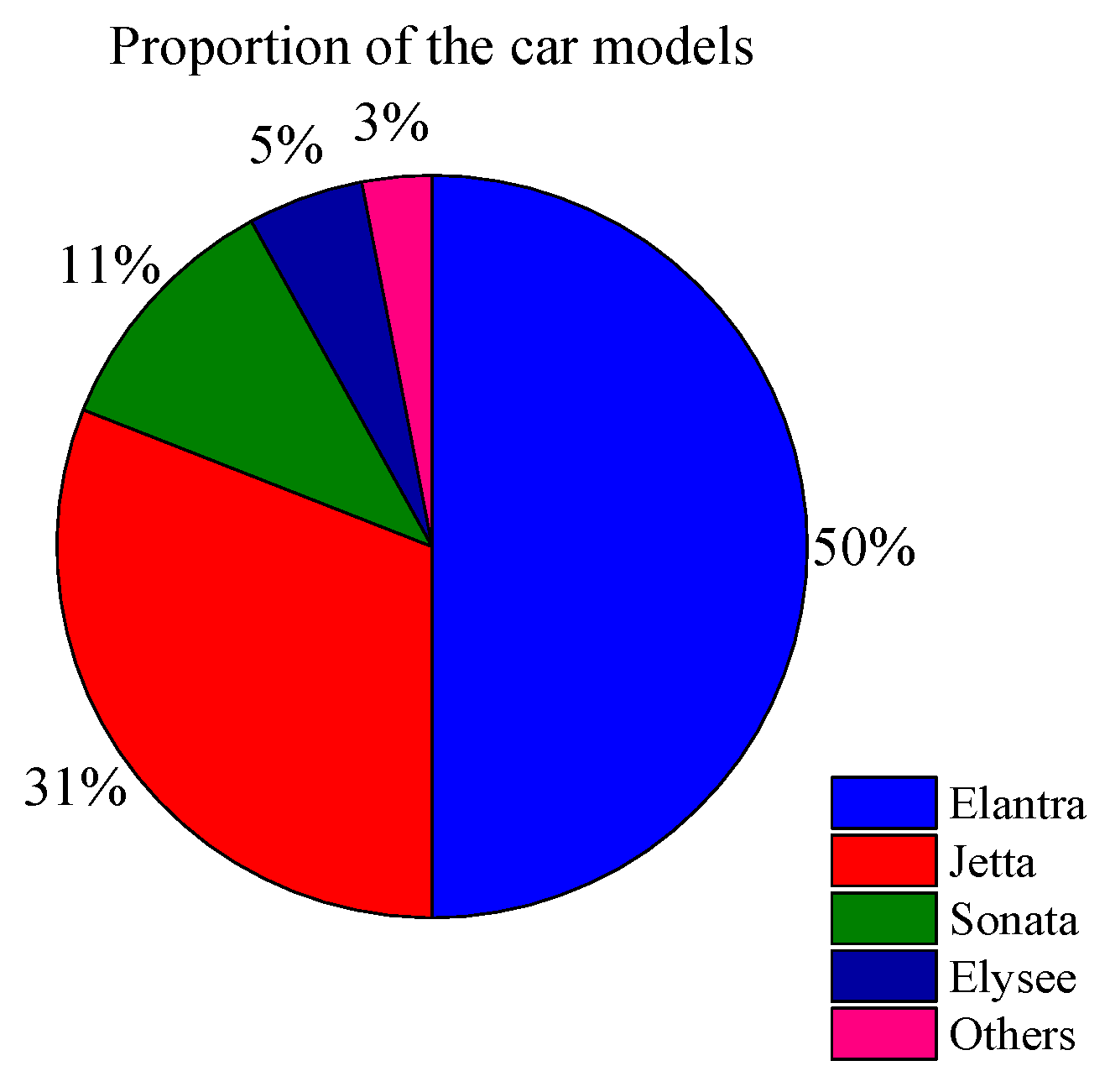
| Car Type | Elantra | Zastava | Santana | Sonata | Citroen | Jetta | Weighted Average |
|---|---|---|---|---|---|---|---|
| number of investigated cars | 40 | 10 | 10 | 10 | 20 | 30 | 120 |
| average FCPOK | 7. 8 | 9. 2 | 8. 5 | 8. 7 | 8. 4 | 8. 1 | 8. 23 |
© 2018 by the authors. Licensee MDPI, Basel, Switzerland. This article is an open access article distributed under the terms and conditions of the Creative Commons Attribution (CC BY) license (http://creativecommons.org/licenses/by/4.0/).
Share and Cite
Zhang, J.; Chen, F.; Wang, Z.; Wang, R.; Shi, S. Spatiotemporal Patterns of Carbon Emissions and Taxi Travel Using GPS Data in Beijing. Energies 2018, 11, 500. https://doi.org/10.3390/en11030500
Zhang J, Chen F, Wang Z, Wang R, Shi S. Spatiotemporal Patterns of Carbon Emissions and Taxi Travel Using GPS Data in Beijing. Energies. 2018; 11(3):500. https://doi.org/10.3390/en11030500
Chicago/Turabian StyleZhang, Jinlei, Feng Chen, Zijia Wang, Rui Wang, and Shunwei Shi. 2018. "Spatiotemporal Patterns of Carbon Emissions and Taxi Travel Using GPS Data in Beijing" Energies 11, no. 3: 500. https://doi.org/10.3390/en11030500
APA StyleZhang, J., Chen, F., Wang, Z., Wang, R., & Shi, S. (2018). Spatiotemporal Patterns of Carbon Emissions and Taxi Travel Using GPS Data in Beijing. Energies, 11(3), 500. https://doi.org/10.3390/en11030500