A Comparison of Thermal Models for Temperature Profiles in Gas-Lift Wells

Abstract
:1. Introduction
2. Methodology
2.1. Assumptions
- (1)
- The thermal conductivity of casing is assumed to be infinity.
- (2)
- The geothermal gradient behind the annulus is not affected by borehole fluid.
- (3)
- Heat capacity of the fluid is constant.
- (4)
- Friction-induced heat is negligible.
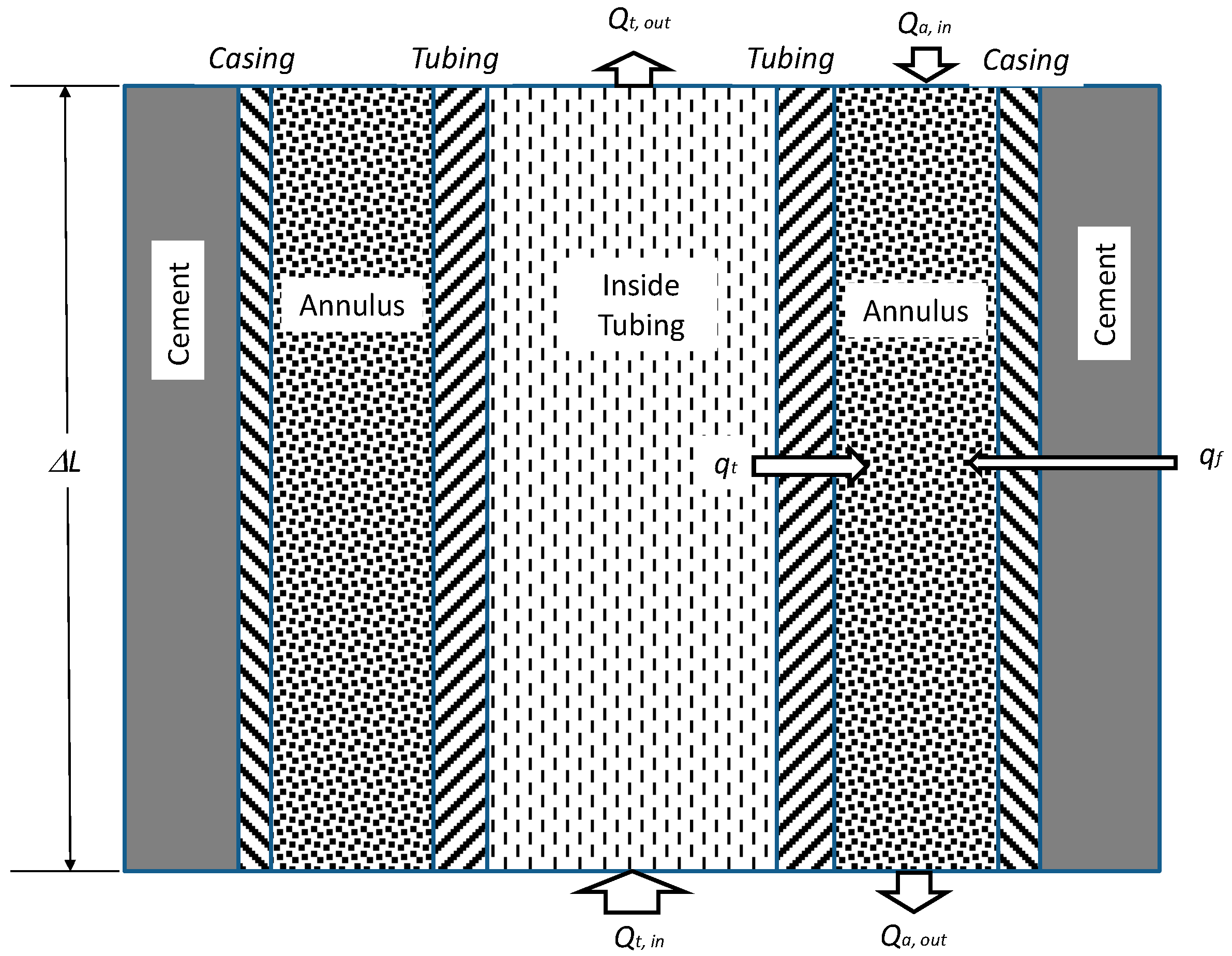
2.2. Governing Equation
2.3. Boundary Conditions
2.4. Analytical Solution
3. Results and Discussion
3.1. Sensitivity Analysis
3.1.1. Sensitivity Analysis Method
3.1.2. Basic Parameters
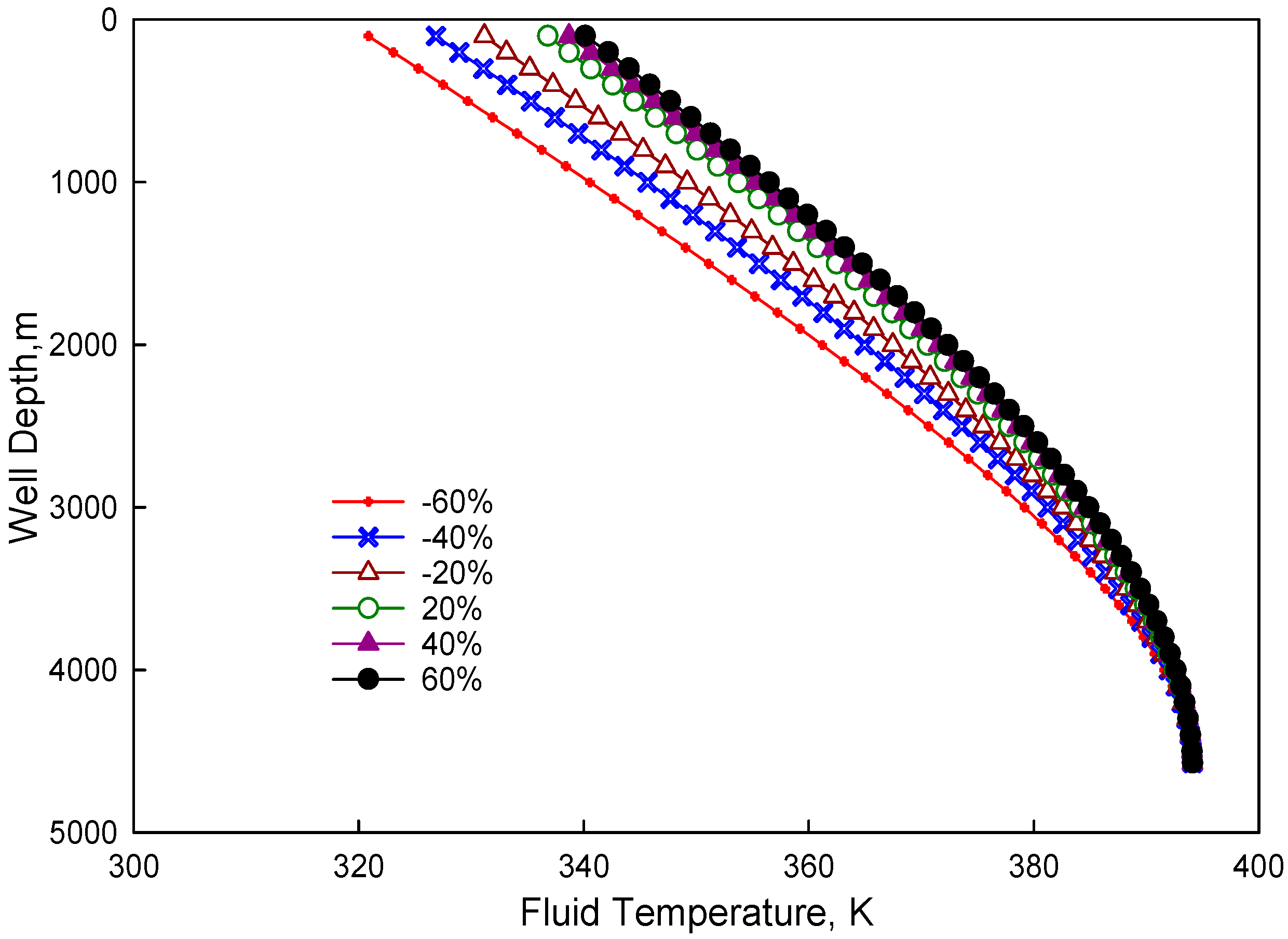
3.1.3. Major Factors Affecting Temperature Distribution inside Tubing
3.1.4. Major Factors Affecting Temperature Distribution in the Annulus
3.2. Case Study
3.2.1. Case 1
3.2.2. Case 2
3.2.3. Case 3
4. Conclusions
- (1)
- A new mechanistic model is developed for computing flowing fluid temperature profiles in both conduits simultaneously for a continuous-flow gas-lift operation. The model assumes steady heat transfer in the formation, as well as steady heat transfer in the conduits. This work also presents a simplified algebraic solution to the analytic model, affording easy implementation in any existing program. An accurate fluid temperature computation should allow improved gas-lift design.
- (2)
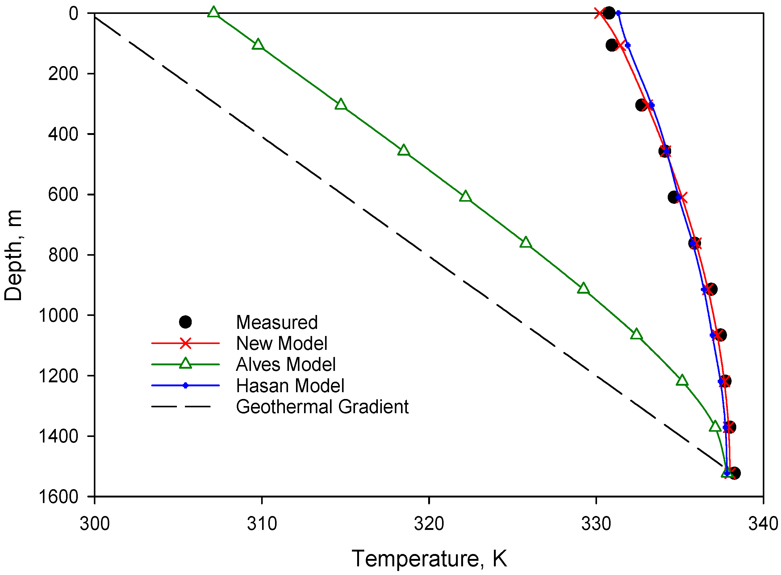
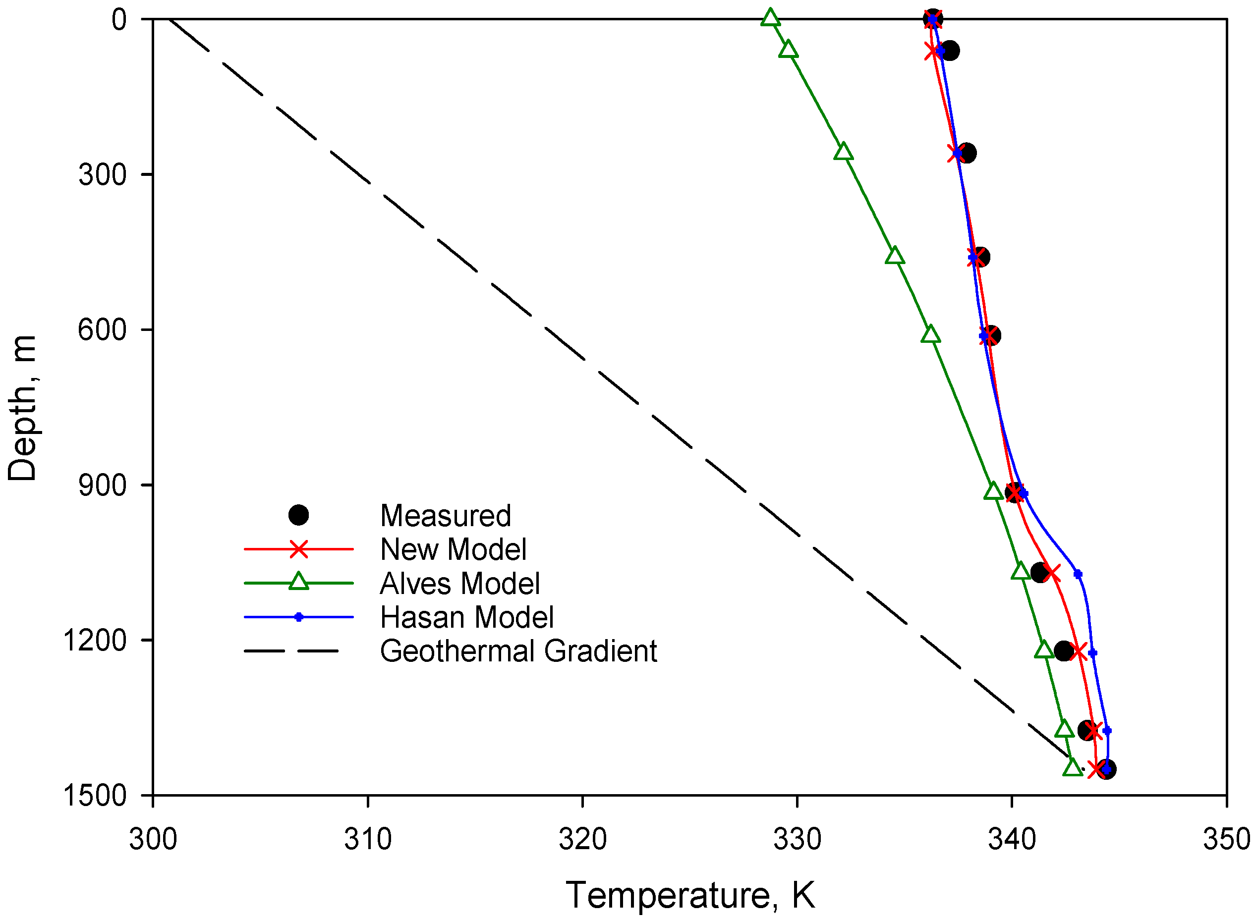
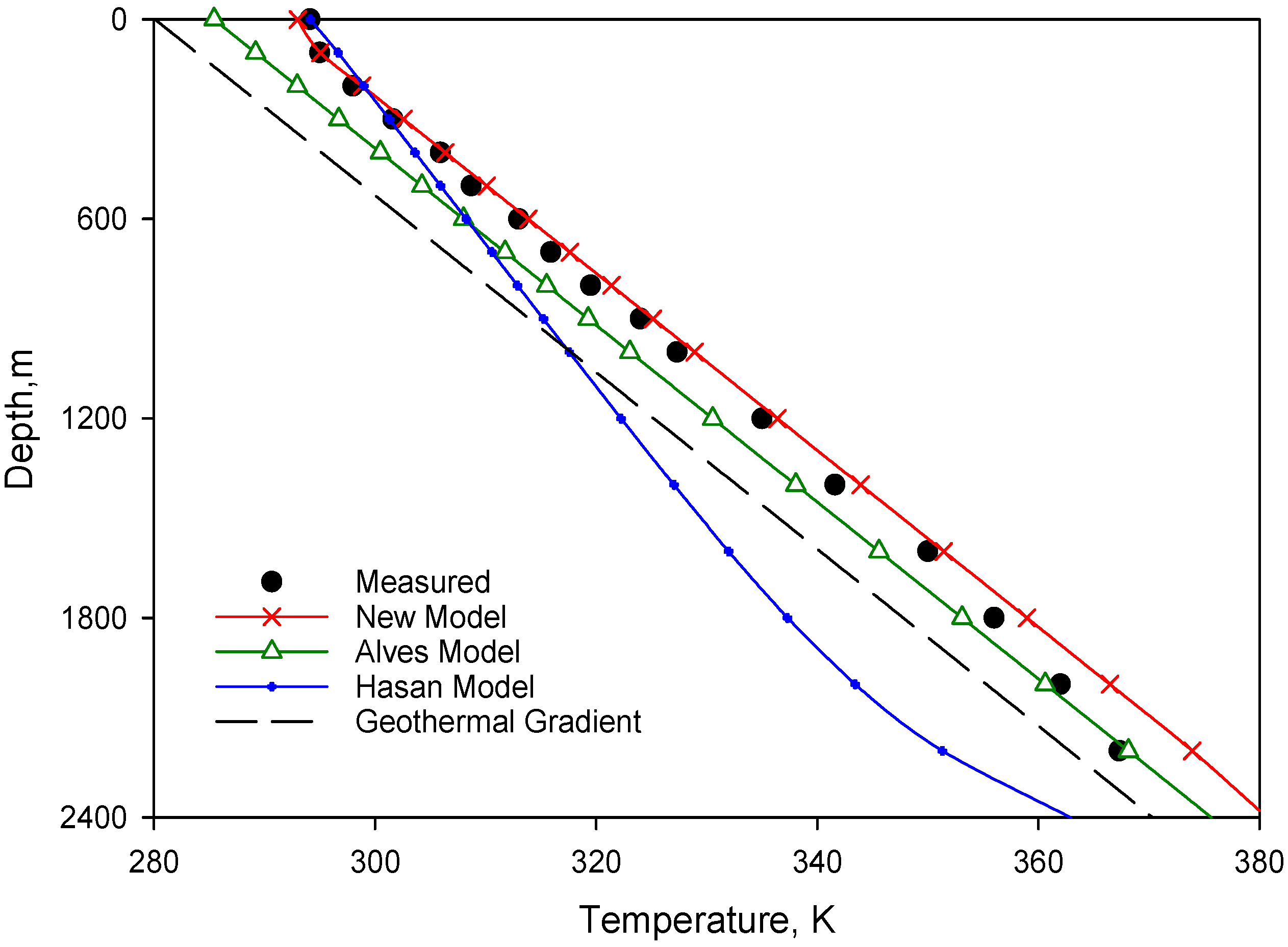
- Comparisons of the Hasan model, Alves model and the new model with data from three actual well show that the temperature profile given by the new model has a better accuracy than that of other models.
- (3)
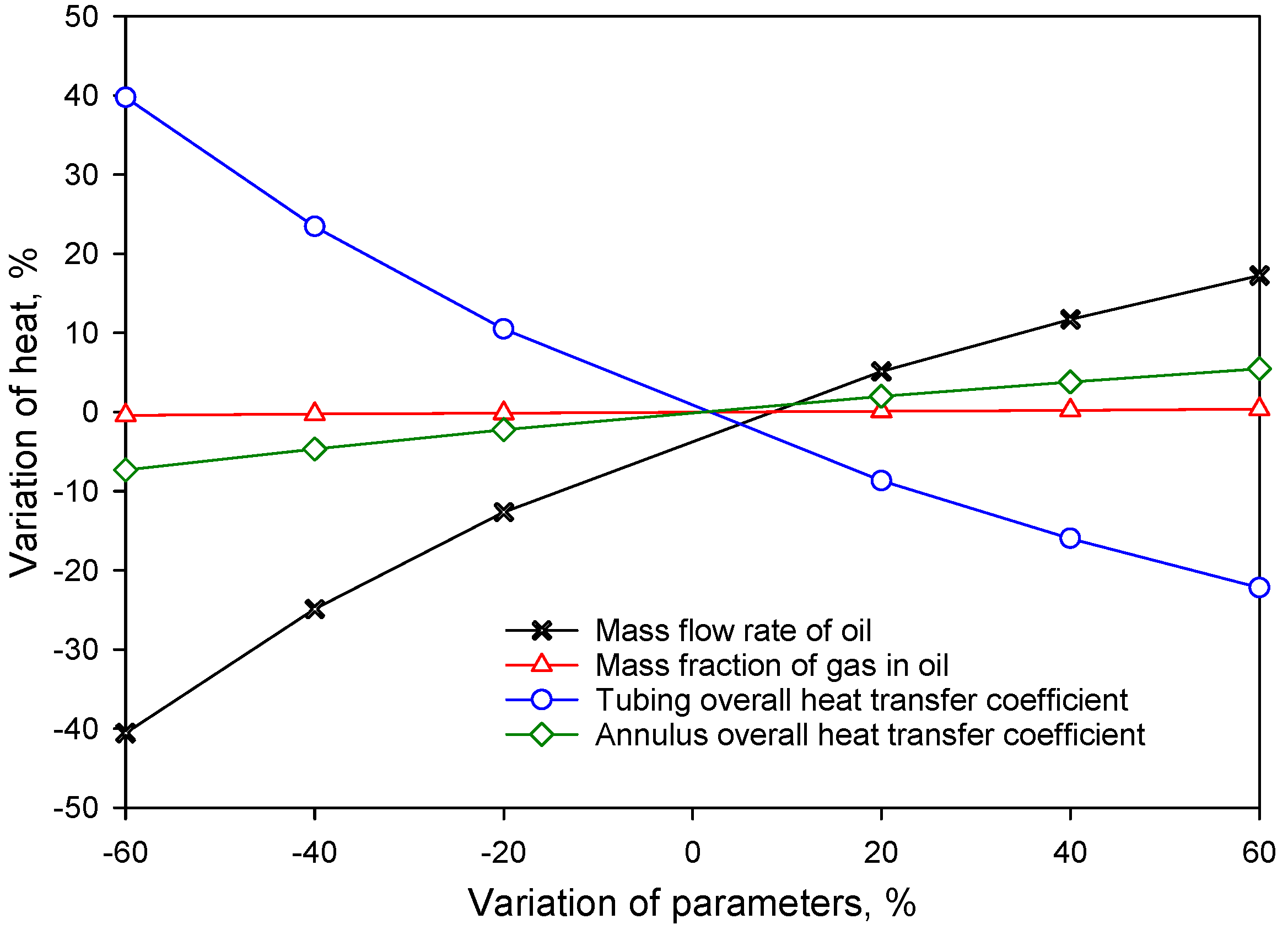
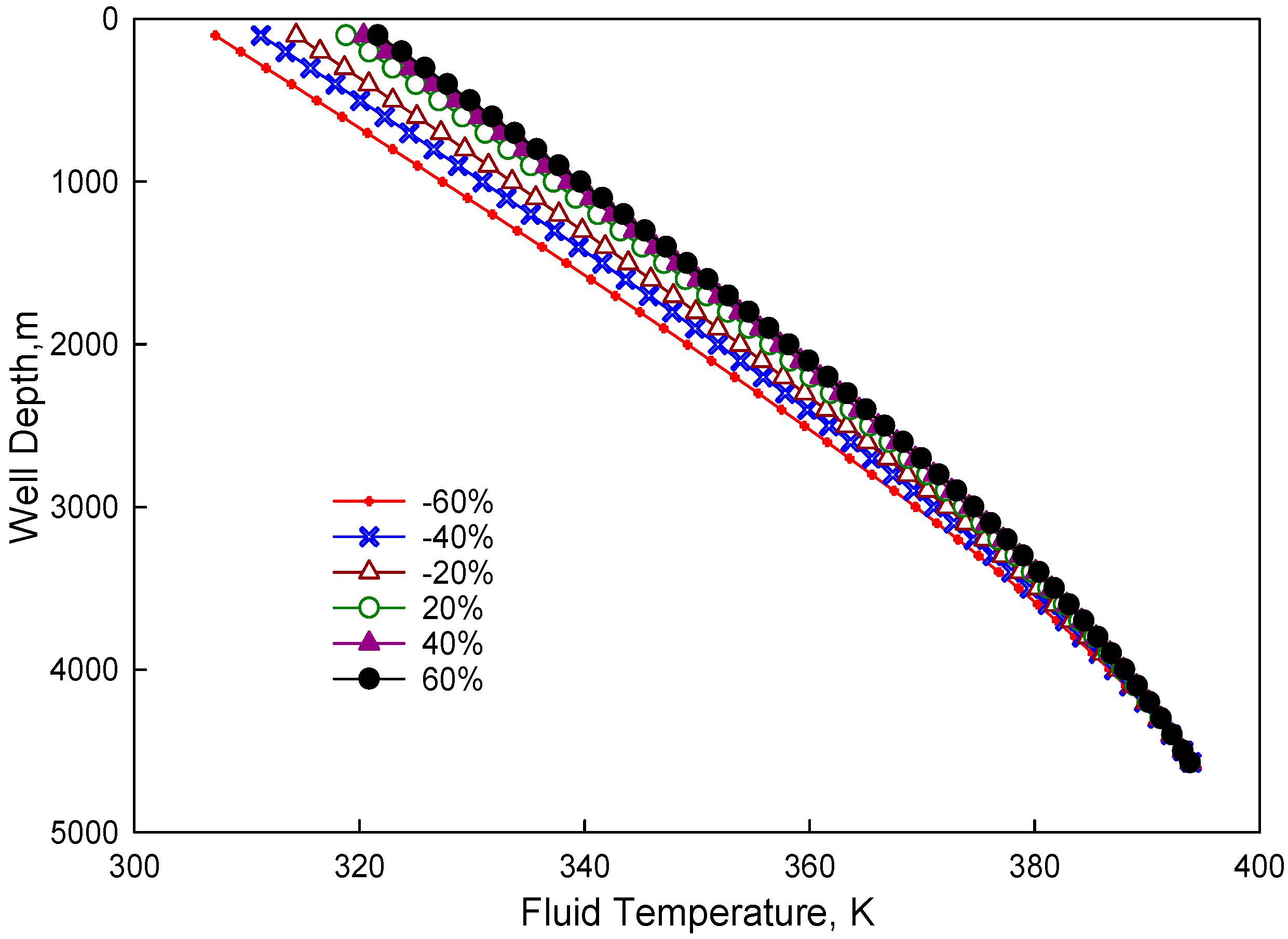
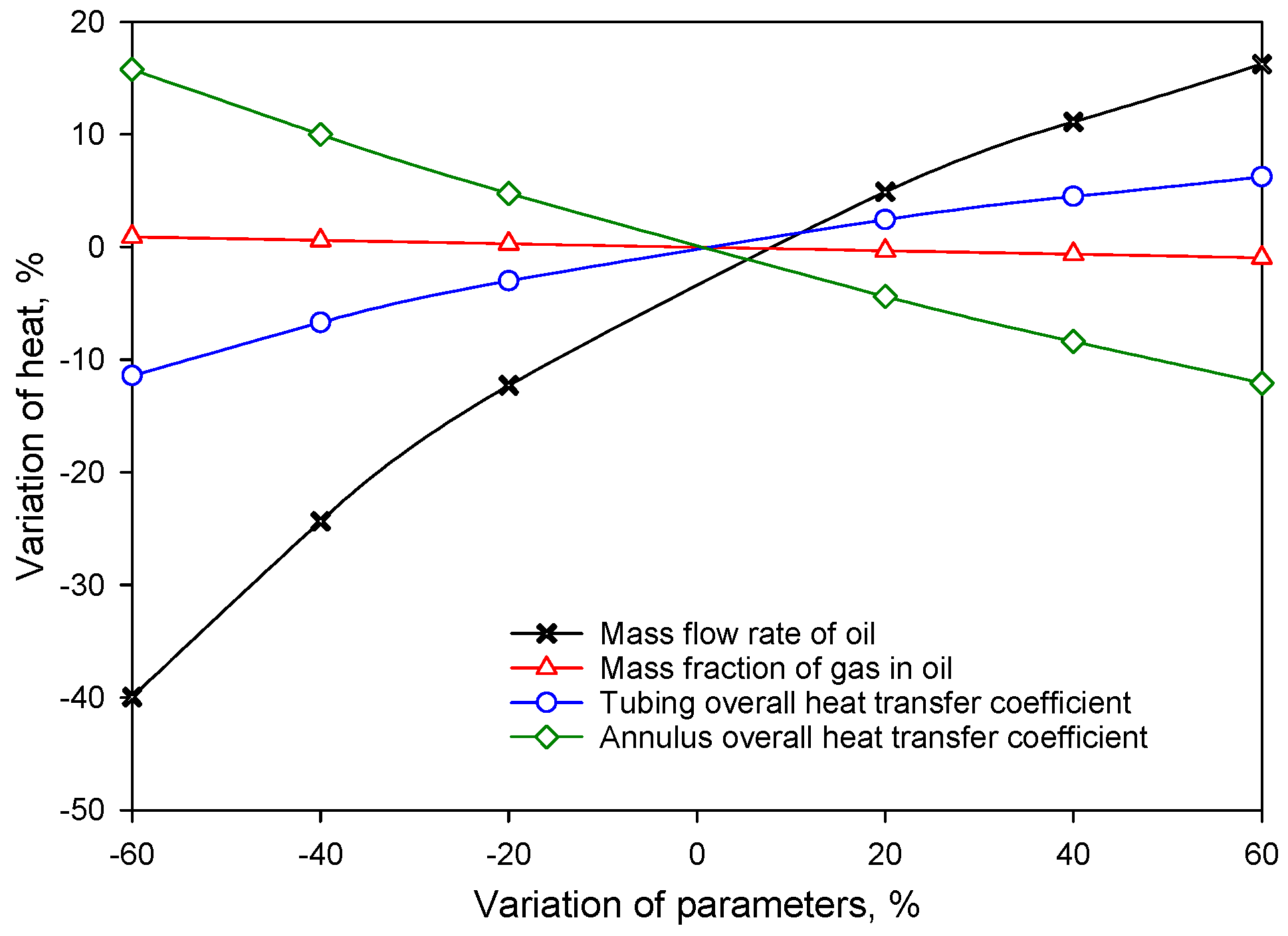
- A sensitivity analysis is conducted with the new model. The results indicate that:
- (a)
- The mass flow rate of oil and the tubing overall heat transfer coefficient are the main factors that influence the temperature distribution inside the tubing;
- (b)
- The mass flow rate of oil is the main factor affecting temperature distribution in the annulus. The annulus overall heat transfer coefficient of the annulus and overall heat transfer coefficient of the tubing are the next factors.
Author Contributions
Conflicts of Interest
Nomenclature
| Ca | the heat capacity of annular fluid |
| Co | the heat capacity of the produced fluid from the oil reservoir |
| Ct | the heat capacity of the tubing fluid |
| dt | the inner diameter of the tubing |
| Dc | the outer diameter of casing |
| Dt | the outer diameter of tubing |
| Dw | the diameter of the wellbore (to sandface) |
| Kt | the thermal conductivity of tubing |
| qf | the heat transfer from the formation rock to the annulus due to conduction |
| qt | heat transfer from the tubing fluid to the annulus due to conduction |
| Qa,in | The heat energy brought into the annular element by the annular fluid due to convection |
| Qa,out | the heat energy carried away from the annular element by the annular fluid due to convection |
| Qa,change | the change of heat energy in the annular fluid in the element |
| Qt,in | the heat energy brought into the tubing element by the tubing fluid due to convection |
| Qt,out | the heat energy carried away from the tubing element by the tubing fluid due to convection |
| Qt,change | the change of heat energy in the tubing fluid in the element |
| r | the radial distant |
| Ta0 | surface temperature, k |
| Ta,L | the temperature of annular fluid at location L |
| Ta,L+ΔL | the temperature of annular fluid at location L + ΔL |
| Tc | the temperature in the cement sheath in the radial direction |
| Tg | the geo-temperature at the depth L |
| TJT | the gas temperature drop due to the Joule–Thomason cooling effect |
| Tt | the temperature of the tubing fluid at the depth L |
| Tt,L+ΔL | the temperature of the tubing fluid at location L + ΔL |
| Ttb | the temperature in the tubing in the radial direction |
| ma | the mass flow rate of annular fluid |
| mo | The mass flow rate of the produced fluid from the oil reservoir |
| mt | the mass flow rate of the tubing fluid |
Appendix A
References
- Clegg, J.D.; Bucaram, S.M.; Hein, N.W., Jr. Recommendation and Comparisons for Selecting Artificial-Lift Methods. J. Pet. Technol. 1993, 45. [Google Scholar] [CrossRef]
- Fleyfel, F.; Meng, W.; Hernandez, O. Production of Waxy Low Temperature Wells with Hot Gas Lift. In Proceedings of the SPE Annual Technical Conference and Exhibition, Houston, TX, USA, 26–29 September 2004; pp. 26–29. [Google Scholar] [CrossRef]
- Aliyeva, F.; Novruzaliyev, B. Gas Lift—Fast and Furious. In Proceedings of the SPE Annual Caspian Technical Conference & Exhibition, Baku, Azerbaijan, 4–6 November 2015; pp. 4–6. [Google Scholar] [CrossRef]
- Guo, B.; Duan, S.; Ghalambor, A. A Simple Model for Predicting Heat Loss and Temperature Profiles in Insulated Pipelines. Soc. Pet. Eng. 2006, 21. [Google Scholar] [CrossRef]
- Muradov, K.M.; Davies, D.R. Novel Analytical Methods of Temperature Interpretation in Horizontal Wells. Soc. Pet. Eng. 2011, 16, 637–647. [Google Scholar] [CrossRef]
- Brown, K.E. The Technology of Artificial Lift Methods; U.S. Department of Energy, Office of Scientific and Technical Information: Oak Ridge, TN, USA, 1984; Volume 4. [Google Scholar]
- Poettmann, F.H.; Carpenter, P.G. The Multiphase Flow of Gas, Oil, and Water through Vertical Flow Strings with Application to the Design of Gas-Lift Installations; American Petroleum Institute: New York, NY, USA, 1952. [Google Scholar]
- Bertuzzi, A.F.; Welchon, J.K.; Poettmann, F.H. Description and Analysis of an Efficient Continuous-Flow Gas-Lift Installation. J. Pet. Technol. 1953, 5, 271–278. [Google Scholar] [CrossRef]
- Hasan, A.R.; Kabir, C.S. Wellbore Heat-Transfer Modeling and Applications. J. Pet. Sci. Eng. 2012, 86, 127–136. [Google Scholar] [CrossRef]
- Gilbertson, E.; Hover, F.; Freeman, B. A Thermally Actuated Gas-lift Safety Valve. SPE Prod. Oper. 2013, 28, 77–84. [Google Scholar] [CrossRef]
- Kirkpatric, C.V. Advanced in Gas Lift Technology; American Petroleum Institute: New York, NY, USA, 1959. [Google Scholar]
- Ramey, H.J., Jr. Wellbore Heat Transmission. J. Pet. Technol. 1962, 14, 427–435. [Google Scholar] [CrossRef]
- Shiu, K.C.; Beggs, H.D. Predicting Temperatures in Flowing Oil Wells. J. Energy Res. Technol. 1980, 102, 2–11. [Google Scholar] [CrossRef]
- Hasan, A.R. A Mechanistic Model for Computing Fluid Temperature Profiles in Gas-Lift Wells. Soc. Pet. Eng. 1996, 11, 179–185. [Google Scholar] [CrossRef]
- Hasan, A.R.; Kabir, C.S.; Lin, D. Analytic Wellbore Temperature Model for Transient Gas-Well Testing. Soc. Pet. Eng. 2005, 8. [Google Scholar] [CrossRef]
- Sagar, R.K.; Doty, D.R.; Schmidt, Z. Predicting Temperature Pro-files in a Flowing Well. SPE Prod. Eng. 1991, 6, 441–448. [Google Scholar] [CrossRef]
- Tartakovsky, A.M.; Ferris, K.F.; Meakin, P. Lagrangian Particle Model for Multiphase Flows. Comput. Phys. Commun. 2009, 180, 1874–1881. [Google Scholar] [CrossRef]
- Farrokhpanah, A.; Bussmann, M.; Mostaghimi, J. New Smoothed Particle Hydrodynamics (SPH) Formulation for Modeling Heat Conduction with Solidification and Melting. Numer. Heat Transf. Part B Fundam. 2017, 71, 299–312. [Google Scholar] [CrossRef]
- Zeng, F.; Zhao, G.; Zhu, L. Detecting CO2 leakage in Vertical Wellbore through Temperature Logging. Fuel 2012, 94, 374–385. [Google Scholar] [CrossRef]
- Alves, I.N.; Alhanati, F.J.S.; Shoham, O. A Unified Model for Predicting Flowing Temperature Distribution in Wellbores and Pipelines. Soc. Pet. Eng. 1992, 7, 363–367. [Google Scholar] [CrossRef]
- Yu, Y.; Lin, T.; Xie, H.; Guan, Y.; Li, K. Prediction of Wellbore Temperature Profiles During Heavy Oil Production Assisted with Light Oil Lift. Soc. Pet. Eng. 2009. [Google Scholar] [CrossRef]
- Lindeberg, E. Modelling Pressure and Temperature Profile in a CO2 Injection well. Energy Procedia 2011, 4, 3935–3941. [Google Scholar] [CrossRef]
- Hamedi, H.; Rashidi, F.; Khamehchi, E. Numerical Prediction of Temperature Profile During Gas Lifting. Pet. Sci. Technol. 2011, 29, 1305–1316. [Google Scholar] [CrossRef]
- Kabir, C.S.; Izgec, B.; Hasan, A.R.; Wang, X. Computing Flow Profiles and Total Flow Rate with Temperature Surveys in Gas Wells. J. Nat. Gas Sci. Eng. 2012, 4, 1–7. [Google Scholar] [CrossRef]
- Duan, J.; Wang, W.; Deng, D.; Zhang, Y.; Liu, H.; Gong, J. Predicting Temperature Distribution in the Waxy Oil-Gas Pipe Flow. J. Pet. Sci. Eng. 2013, 101, 28–34. [Google Scholar] [CrossRef]
- Cheng, W.L.; Nian, Y.L.; Li, T.T.; Wang, C.L. A Novel Method for Predicting Spatial Distribution of Thermal Properties and Oil Saturation of Steam Injection Well from Temperature Logs. Energy 2014, 66, 898–906. [Google Scholar] [CrossRef]
- Han, G.; Zhang, H.; Ling, K.; Wu, D.; Zhang, Z. A Transient Two-Phase Fluid- and Heat-Flow Model for Gas-Lift-Assisted Waxy-Crude Wells with Periodical Electric Heating. Soc. Pet. Eng. 2014, 53. [Google Scholar] [CrossRef]
- Hasan, A.R.; Kabir, C.S.; Wang, X. A Robust Steady-State Model for Flowing-Fluid Temperature in Complex Wells. Soc. Pet. Eng. 2009, 24, 269–276. [Google Scholar] [CrossRef]
- Wei, L.; Qian, Y. New Prediction Model for Temperature Distribution in Gas Lift Annulus Hot Gas Injection Wellbore. Oil Gas Field Dev. 2014, 32, 41–44. [Google Scholar]


| Coefficient | Value | ||
|---|---|---|---|
| (low) | (High) | (Average) | |
| Well depth, m | ------ | ------ | 4572 |
| Casing radius, m | ------ | ------ | 0.11 |
| Tubing radius, m | ------ | ------ | 0.07 |
| Mass flow rate of oil, kg/s | 0.74 | 15.88 | 8.31 |
| Mass fraction of gas in oil | 0.05 | 0.10 | 0.075 |
| Specific heat of oil, J/(kg·K) | ------ | ------ | 1674.72 |
| Specific heat of gas, J/(kg·K) | ------ | ------ | 1046.7 |
| Tubing overall heat transfer coefficient, W/(m2·K) | 28.39 | 113.57 | 70.98 |
| Annulus overall heat transfer coefficient, W/(m2·K) | 11.36 | 22.71 | 17.03 |
| Geothermal gradient, K/m | ------ | ------ | 0.0427 |
| Bottomhole earth temperature, K | ------ | ------ | 394.26 |
| Surface earth temperature, K | ------ | ------ | 288.43 |
| Surface gas inlet temperature, K | ------ | ------ | 318.15 |
| Variation of Parameters | Mass Flow Rate of Oil | Mass Fraction of Gas in Oil | Tubing Overall Heat Transfer Coefficient | Annulus Overall Heat Transfer Coefficient |
|---|---|---|---|---|
| −60% | 3.76 | 0.060 | 45.43 | 13.63 |
| −40% | 5.28 | 0.065 | 53.94 | 14.76 |
| −20% | 6.79 | 0.070 | 62.46 | 15.90 |
| 20% | 9.82 | 0.080 | 79.49 | 18.17 |
| 40% | 11.33 | 0.085 | 88.02 | 19.31 |
| 60% | 12.85 | 0.090 | 96.53 | 20.44 |
| Parameter Variations | Mass Flow Rate of Oil | Mass Fraction of Gas in Oil | Tubing Overall Heat Transfer Coefficient | Annulus Overall Heat Transfer Coefficient |
|---|---|---|---|---|
| −60% | 46.06% | 0.43% | 45.17% | 8.34% |
| −40% | 46.79% | 0.48% | 44.03% | 8.71% |
| −20% | 49.62% | 0.50% | 41.24% | 8.64% |
| 20% | 32.21% | 0.80% | 54.47% | 12.52% |
| 40% | 36.89% | 0.80% | 50.30% | 12.01% |
| 60% | 38.07% | 0.85% | 48.99% | 12.09% |
| Parameter Variations | Mass Flow Rate of Oil | Mass Fraction of Gas in Oil | Tubing Overall Heat Transfer Coefficient | Annulus Overall Heat Transfer Coefficient |
|---|---|---|---|---|
| −60% | 58.70% | 1.36% | 16.77% | 23.18% |
| −40% | 58.46% | 1.48% | 16.05% | 24.01% |
| −20% | 60.33% | 1.52% | 14.68% | 23.47% |
| 20% | 40.80% | 2.57% | 20.37% | 36.27% |
| 40% | 45.19% | 2.51% | 18.29% | 34.01% |
| 60% | 45.80% | 2.61% | 17.58% | 34.01% |
| Coefficient | Value |
|---|---|
| Total well depth, m | 1529.79 |
| Depth of gas infection, m | 731.52 |
| Casing ID, m | 0.18 |
| Tubing OD, m | 0.073 |
| Oil + water flow rate, m3/s | 0.0038 |
| Mass fraction of gas in the tubing | 0.0681 |
| Gas/liquid ratio, m3/m3 | 97.9 |
| Oil + water API gravity | 10.3 |
| Gas gravity (air = 1) | 0.61 |
| Specific heat of liquid, J/(kg·K) | 4186.8 |
| Specific heat of gas, J/(kg·K) | 1046.7 |
| Tubing overall heat transfer coefficient, W/(m2·K) | 56.78 (Hasan and Alves), 39.75 (New model) |
| Annulus overall heat transfer coefficient, W/(m2·K) | 22.71 |
| Earth thermal conductivity, W/(m·K) | 2.25 |
| Geothermal gradient, K/m | 0.045 |
| Bottomhole earth temperature, K | 338.15 |
| Surface earh temperature, K | 299.82 |
| Surface gas inlet temperature, K | 310.93 |
| Coefficient | Value |
|---|---|
| Total well depth, m | 1517.5992 |
| Depth of gas infection, m | 673.303 |
| Casing ID, m | 0.127 |
| Tubing OD, m | 0.0635 |
| Oil + water flow rate, m3/s | 0.00674 |
| Mass fraction of gas in the tubing | 0.0225 |
| Gas/liquid ratio, m3/m3 | 28.124 |
| Oil + water API gravity | 26 |
| Gas gravity (air = 1) | 0.60 |
| Specific heat of liquid, J/(kg·K) | 4186.8 |
| Specific heat of gas, J/(kg·K) | 1046.7 |
| Tubing overall heat transfer coefficient, W/(m2·K) | 56.78 (Hasan and Alves), 45.43 (New model) |
| Annulus overall heat transfer coefficient, W/(m2·K) | 5.68 (Hasan and Alves), 9.65 (New model) |
| Earth thermal conductivity, W/(m·K) | 2.25 |
| Geothermal gradient, K/m | 0.0522 |
| Bottomhole earth temperature, K | 344.8 |
| Surface earh temperature, K | 300.93 |
| Surface gas inlet temperature, K | 310.93 |
| Coefficient | Value |
|---|---|
| Depth of oil layer, m | 2691.01 |
| Temperature in the mid-layer, K | 399.07 |
| Relative density of crude oil | 0.8375 |
| Relative density of output gas | 0.7103 |
| Proportion of injected gas | 0.65 |
| Tubing size, m | 0.073 |
| Casing size, m | 0.178 |
| Geothermal gradient, K/m | 0.068 |
| Injected point, m | 2511.13 |
| Gas injection volume, m3/s | 0.092 |
| Liquid production volume, m3/s | 0.0001414 |
| Oil production, m3/s | 0.000113 |
| Gas production, m3/s | 0.139 |
| Moisture content/(%) | 19.9 |
| Temperature of injected gas, K | 313.15 |
© 2018 by the authors. Licensee MDPI, Basel, Switzerland. This article is an open access article distributed under the terms and conditions of the Creative Commons Attribution (CC BY) license (http://creativecommons.org/licenses/by/4.0/).
Share and Cite
Mu, L.; Zhang, Q.; Li, Q.; Zeng, F. A Comparison of Thermal Models for Temperature Profiles in Gas-Lift Wells. Energies 2018, 11, 489. https://doi.org/10.3390/en11030489
Mu L, Zhang Q, Li Q, Zeng F. A Comparison of Thermal Models for Temperature Profiles in Gas-Lift Wells. Energies. 2018; 11(3):489. https://doi.org/10.3390/en11030489
Chicago/Turabian StyleMu, Langfeng, Qiushi Zhang, Qi Li, and Fanhua Zeng. 2018. "A Comparison of Thermal Models for Temperature Profiles in Gas-Lift Wells" Energies 11, no. 3: 489. https://doi.org/10.3390/en11030489
APA StyleMu, L., Zhang, Q., Li, Q., & Zeng, F. (2018). A Comparison of Thermal Models for Temperature Profiles in Gas-Lift Wells. Energies, 11(3), 489. https://doi.org/10.3390/en11030489