Real-Time Genetic Algorithms-Based MPPT: Study and Comparison (Theoretical an Experimental) with Conventional Methods

Abstract

Maximum Power Point Tracking (MPPT) methods are used in photovoltaic (PV) systems to continually maximize the PV array output power, which strongly depends on both solar radiation and cell temperature. The PV power oscillations around the maximum power point (MPP) resulting from the conventional methods and complexity of the non-conventional ones are convincing reasons to look for novel MPPT methods. This paper deals with simple Genetic Algorithms (GAs) based MPPT method in order to improve the convergence, rapidity, and accuracy of the PV system. The proposed method can also efficiently track the global MPP, which is very useful for partial shading. At first, a review of the algorithm is given, followed with many test examples; then, a comparison by means Matlab/Simulink© (R2009b) is conducted between the proposed MPPT and, the popular Perturb and Observe (PO) and Incremental Conductance (IC) techniques. The results show clearly the superiority of the proposed controller. Indeed, with the proposed algorithm, oscillations around the MPP are dramatically minimized, a better stability is observed and increase in the output power efficiency is obtained. All these results are experimentally validated by a test bench developed at LIAS laboratory (Poitiers University, Poitiers, France) using real PV panels and a PV emulator which allows one to define a profile insolation model. In addition, the proposed method permits one to perform the test of linearity between the optimal current ${\mathrm{I}}_{\mathrm{mp}}$ (current at maximum power) and the short-circuit current ${\mathrm{I}}_{\mathrm{sc}}$, and between the optimal voltage ${\mathrm{V}}_{\mathrm{mp}}$ and open-circuit voltage ${\mathrm{V}}_{\mathrm{oc}}$, so the current and voltage factors can be easily obtained with our algorithm.

1. Introduction

PV energy has been widely used during recent years because of its advantages, the growth in the world demand of energy, and the lowering of the PV panels’ cost [1].

The PV output power efficiency is low and can be even lower if the panels do not operate at their MPP, but this changes with atmospheric conditions (insolation and temperature) so it is very important to ensure the panels operate around that point.

Many methods are used to track the MPP, they can be divided in two groups: conventional and non-conventional methods. The conventional methods are widely used (such as Perturb and Observe (PO) [2,3], Incremental Conductance (IC) [4,5]) because they are simple and easy to implement. But, both the PO and IC methods result in oscillation of power around the MPP because the perturbation remains even when the system operates at MPP. This problem can be reduced by decreasing the step of the duty cycle. But in this case, the algorithm will track the MPP slowly in response to changing atmospheric conditions, leading to more power loss. Another solution based on variable duty cycle step is proposed [6,7].

In addition, the two previously mentioned conventional techniques may converge to a local optimum which is not necessarily the real MPP. Indeed, the search technique of these algorithms is done point by point and the P–V curve can present more than one optimum in case of partial shading.

The linear method [8,9] is also widely used due to its simplicity. It assumes a linear relation between ${\mathrm{I}}_{\mathrm{mp}}$ and ${\mathrm{I}}_{\mathrm{sc}}$ (current factor ${\mathrm{M}}_{\mathrm{c}}$), and between ${\mathrm{V}}_{\mathrm{mp}}$ and ${\mathrm{V}}_{\mathrm{oc}}$ (voltage factor ${\mathrm{M}}_{\mathrm{V}}$), but these relations are not absolutely linear because of the nonlinear cell model and because of the temperature and the insolation dependency of ${\mathrm{M}}_{\mathrm{c}}$ and ${\mathrm{M}}_{\mathrm{V}}$. With the proposed algorithm, both ${\mathrm{I}}_{\mathrm{sc}}$ and ${\mathrm{V}}_{\mathrm{oc}}$ are measured (including insolation and temperature effect) and the nonlinear cell model is really used.

Many investigations about non-conventional MPPT methods have been presented (fuzzy logic [10,11], sliding-mode [12], neural-network [13], ...) during the last decade. They give interesting theoretical results, but their complexity needs much knowledge, making their implementation very difficult.

A good review and comparison of MPPT methods for PV systems under normal and partial shading conditions is given by Ramli et al. [14]. Kamarzaman & Tan [15] made a short theoretical review comparison between conventional MPPT and stochastic based MPPT algorithms and showed an interesting performance of GAs-based MPPT. Daraban et al. [16] used GAs with an embedded PO algorithm, which slightly reduces the oscillations, although they remain important. Logeswarana & SenthilKumar [17] introduced a re-initialization step to avoid a local convergence.

The proposed algorithm needs short-circuit current ${\mathrm{I}}_{\mathrm{sc}}$ and open-circuit voltage ${\mathrm{V}}_{\mathrm{oc}}$ as inputs and uses the cell model to find the MPP (not using perturbation step), so it can rapidly track the variation of climatic conditions (temperature and insolation). The genetic parameters are chosen to ensure a large diversity. In order to improve the rapidity of the controller and avoid a local optimum, it is important to choose a suitable fitness function. In this paper, the fitness function is extracted from the PV cell model (PV power) in order to give a greater opportunity to the optimal individuals and to not completely eliminate the others. To validate the performance of the proposed algorithm, theoretical (by using Matlab/Simulink (R2009b)) and experimental (by using real panels) comparison with the PO and IC methods is given. The algorithm works by global tracking using a population of points instead of only one (case of IC and PO). This can avoid the problem of convergence to the local optimum. Even better, the problem of power oscillation around the MPP can be solved.

Using the proposed algorithm, the linear method is verified, and the factors ${\mathrm{M}}_{\mathrm{c}}$ and ${\mathrm{M}}_{\mathrm{V}}$ can be easily obtained.

2. Conventional Methods

2.1. PO and IC Algorithms

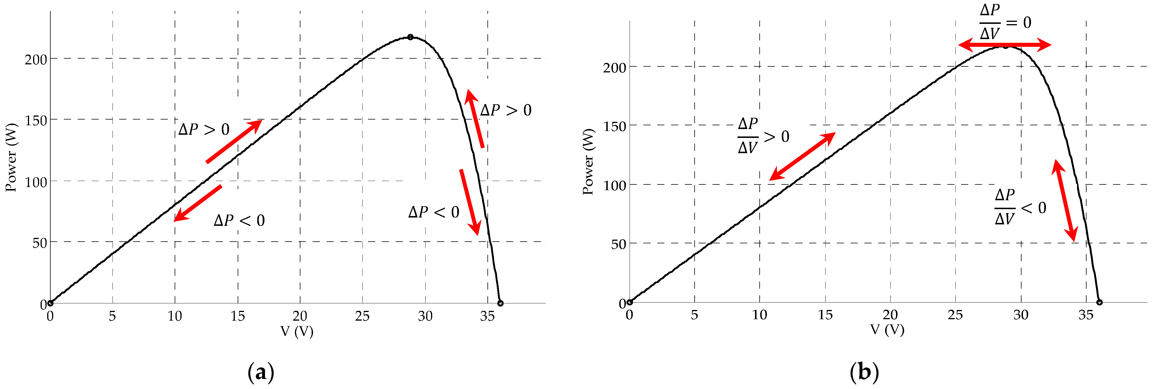
With PO [2,3], the MPP tracking operates by perturbing (i.e., incrementing or decrementing the duty cycle) the array terminal voltage and comparing the PV output power and voltage values with the previous cycle values. If the PV output power increases ($\Delta \mathrm{P}>0$), the perturbation will continue with the same direction in the next cycle, otherwise ($\Delta \mathrm{P}<0$) the perturbation direction will be reversed (Figure 1a).

Various PO algorithms are widely used in MPPT because of their simple structure and the requirement for few measured parameters. Therefore, when the MPP is reached, the PO algorithm will oscillate around it, resulting in a loss of PV power. Also, by taking just the power variation (∆P), in rapidly changing atmospheric conditions the PO algorithm can deviate from the MPP and search in the wrong direction. This can be solved by the IC method by considering the power derivation ($\mathrm{dP}/\mathrm{dV}$).

Power derivation allows one to track the MPP with the real direction because $\mathrm{dP}/\mathrm{dV}$ informs us about the operating point (Figure 1b) at the right or the left of MPP. The derivation of power can be written: $\frac{\mathrm{dP}}{\mathrm{dV}}=\frac{\mathrm{d}\left(\mathrm{I}·\mathrm{V}\right)}{\mathrm{dV}}=\mathrm{V}·\frac{\mathrm{dI}}{\mathrm{dV}}+\mathrm{I}$, so at MPP we can write:

$$\frac{\mathrm{dP}}{\mathrm{dV}}=0\Rightarrow \frac{\mathrm{dI}}{\mathrm{dV}}=-\frac{\mathrm{I}}{\mathrm{V}},$$

(1)

We can see that the MPP is given by comparing the incremental and instantaneous conductance:

• $\frac{\mathrm{dI}}{\mathrm{dV}}>-\frac{\mathrm{I}}{\mathrm{V}}\to$ Increase PV array voltage (V)
• $\frac{\mathrm{dI}}{\mathrm{dV}}<-\frac{\mathrm{I}}{\mathrm{V}}\to$ Decrease V
• $\frac{\mathrm{dI}}{\mathrm{dV}}\approx -\frac{\mathrm{I}}{\mathrm{V}}\leftrightarrow$ At the MPP

This algorithm can rapidly follow the variation of atmospheric conditions, but by trying to obtain $\mathrm{dP}/\mathrm{dV}=0$ makes it sensitive to the perturbations.

2.2. The Linear Method

This method [8,9] assumes a linear relation between the optimal current ${\mathrm{I}}_{\mathrm{mp}}$ (current at maximum power) and the short-circuit current ${\mathrm{I}}_{\mathrm{sc}}$, and between the optimal voltage ${\mathrm{V}}_{\mathrm{mp}}$ and open-circuit voltage ${\mathrm{V}}_{\mathrm{oc}}$, so we can write:

$${\mathrm{I}}_{\mathrm{mp}}={\mathrm{M}}_{\mathrm{c}}·{\mathrm{I}}_{\mathrm{sc}},$$

(2)

$${\mathrm{V}}_{\mathrm{mp}}={\mathrm{M}}_{\mathrm{V}}·{\mathrm{V}}_{\mathrm{oc}}$$

(3)

where ${\mathrm{M}}_{\mathrm{c}}$ and ${\mathrm{M}}_{\mathrm{V}}$ are constants.

Using a pilot cell, one can measure ${\mathrm{I}}_{\mathrm{sc}}$ and ${\mathrm{V}}_{\mathrm{oc}}$ and find the MPP. This method is very simple and gives acceptable results, however the two factors are not a constant because of the nonlinear cell model.

3. The Proposed Method

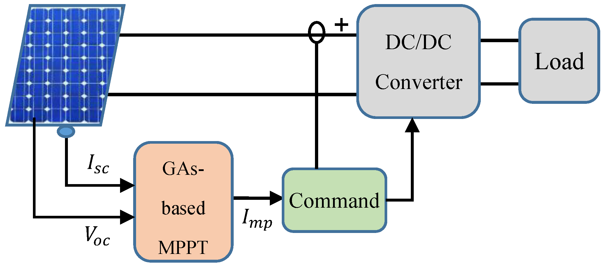
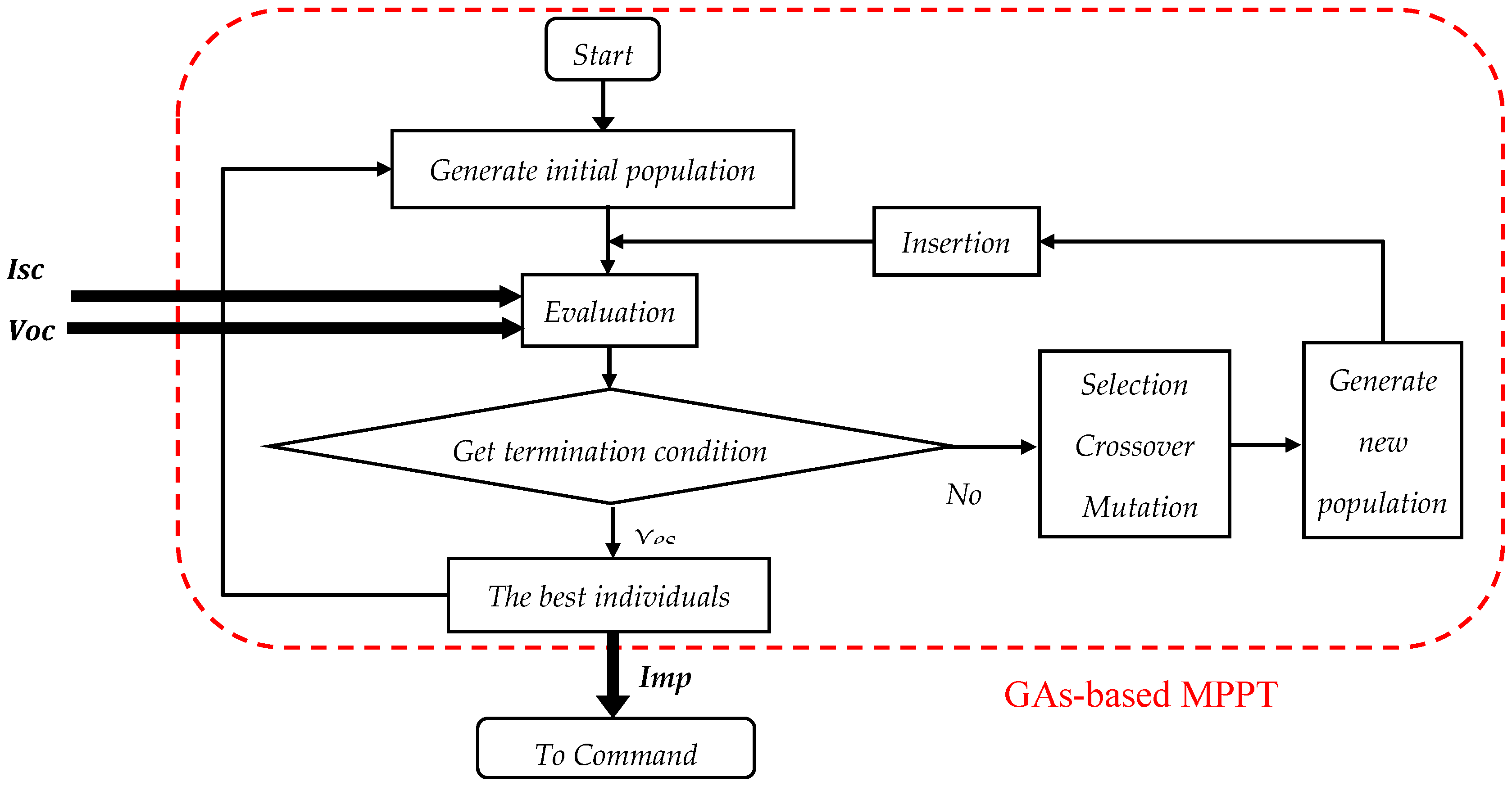
MPPT techniques try to track the optimum point corresponding to the maximum PV power, this point is defined by an optimum current ${\mathrm{I}}_{\mathrm{mp}}$ (current at maximum power). By using GAs, one can find this current and keep PV panels working around the maximum power. Figure 2 depicts the GAs-based MPPT PV system.

The main idea is to perform genetic transformations (Selection, crossover, mutation, and insertion) on a population of individuals in order to finally obtain an optimal individual corresponding to the maximum of a function (fitness function) [18]. The following flow chart (Figure 3) shows the steps of the algorithm:

3.1. Initialization

In our Algorithm, the initial population is a binary matrix which is randomly created. It contains N individuals (photovoltaic current) coded on S bits:

$$\mathrm{population}\left(\mathrm{I}\right)=\left[\begin{array}{c}{\mathrm{I}}_1\\ ⋮\\ {\mathrm{I}}_{\mathrm{N}}\end{array}\right]\mathrm{With}:{\mathrm{I}}_{\max }={\mathrm{I}}_{\mathrm{sc}}=111\dots 11$$

So, $\mathrm{population}\left(\mathrm{I}\right)=\left[\begin{array}{ccc}& \cdots & \\ ⋮& \ddots & ⋮\\ & \cdots & \end{array}\right]$.

The effect of the number of bits (S) and the population length (N) is discussed on Section 4. The created population will be evaluated according to the power (fitness) of each individual.

3.2. Evaluation

The evaluation is a very important operation; it ensures the survival of an optimal individual. This can be done by the fitness function (it is a positive function and the individual is optimized for the maximum value of its fitness function). In our case, the fitness function is simply the PV power, so the optimal individual gives the maximum power. An evaluation of each individual (PV current) is given according to the corresponding power:

$$\mathrm{P}=\mathrm{V}·\mathrm{I},$$

(4)

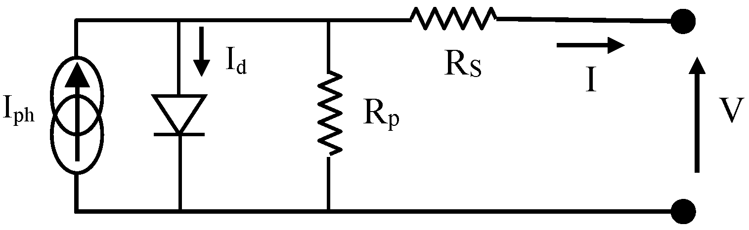
The cell model, shown by the circuit in Figure 4, is used to evaluate the power of each individual (fitness function), where $\mathrm{Rp}$ and $Rs$ are the series and parallel resistances of the cell, respectively [19,20].

Usually the value of $\mathrm{Rp}$ is very high, so the equation for the output current can be given by:

$$\mathrm{I}={\mathrm{I}}_{\mathrm{ph}}-{\mathrm{I}}_{\mathrm{d}},$$

(5)

with:

$${\mathrm{I}}_{\mathrm{d}}={\mathrm{I}}_{\mathrm{rs}}\left[e^{\left(\frac{\mathrm{q}}{\mathrm{kTA}}\left(\mathrm{V}+{\mathrm{R}}_{\mathrm{s}}\mathrm{I}\right)\right)}-1\right],$$

(6)

where: $\mathrm{I}$: Output current (A); $\mathrm{V}$: Output Voltage (V); I_d: Current through the intrinsic diode; I_ph: Cell photocurrent; I_rs: Cell reverse saturation current; $\mathrm{q}$: The charge of an electron; $\mathrm{k}$: Bolzmann’s constant; $\mathrm{A}$: The p–n junction ideality factor; $\mathrm{T}$: Cell temperature (K); $\mathrm{Rs}$: Series resistances of the cell (Ω).

Making the approximation that I_ph $\approx$ I_sc where $\mathrm{Isc}$ is short-circuit current, (5) becomes:

$$\mathrm{I}={\mathrm{I}}_{\mathrm{sc}}-{\mathrm{I}}_{\mathrm{rs}}\left[e^{\left(\frac{\mathrm{V}+{\mathrm{R}}_{\mathrm{s}}\mathrm{I}}{{\mathrm{V}}_{\mathrm{T}}}\right)}-1\right],$$

(7)

where:

$${\mathrm{V}}_{\mathrm{T}}=\frac{\mathrm{kTA}}{\mathrm{q}},$$

(8)

At open circuit: $\mathrm{I}=0$ and $\mathrm{V}=$ V_oc, with V_oc is open-circuit voltage; Using (7), we can write:

$${\mathrm{I}}_{\mathrm{rs}}=\frac{{\mathrm{I}}_{\mathrm{sc}}}{e^{\left(\frac{{\mathrm{V}}_{\mathrm{oc}}}{{\mathrm{V}}_{\mathrm{T}}}\right)}-1},$$

(9)

Using (7) and (9), the output voltage equation of the cell will be:

$$\mathrm{V}={\mathrm{V}}_{\mathrm{T}}\mathrm{Ln}\left[\left(1-\frac{\mathrm{I}}{{\mathrm{I}}_{\mathrm{sc}}}\right)\left(e^{\left(\frac{{\mathrm{V}}_{\mathrm{oc}}}{{\mathrm{V}}_{\mathrm{T}}}\right)}-1\right)+1\right]-{\mathrm{R}}_{\mathrm{s}}\mathrm{I},$$

(10)

Finally, the power equation can be given with (4) and (10):

$$\mathrm{P}=\left({\mathrm{V}}_{\mathrm{T}}\mathrm{Ln}\left[\left(1-\frac{\mathrm{I}}{{\mathrm{I}}_{\mathrm{sc}}}\right)\left(e^{\left(\frac{{\mathrm{V}}_{\mathrm{oc}}}{{\mathrm{V}}_{\mathrm{T}}}\right)}-1\right)+1\right]-{\mathrm{R}}_{\mathrm{s}}\mathrm{I}\right)·\mathrm{I},$$

(11)

Using this equation, power (fitness function) is calculated for each individual and this value will be used in genetic operations to create a new population (generation) and this one will be inserted in the parent population according to their fitness function.

3.3. Genetic Operations

Genetic operations are the base of GAs; they do not exclude probability theories, but they give very interesting results. These operations are:

• Selection: Select, with a rate T_sel $(\%)$, a part of the population corresponding to the optimum fitness; in nature, only the individuals more adapted to the environment will survive. The roulette wheel selection method is used.
• Crossover: After selection, natural reproduction is performed by crossing pairs of individuals.
• Mutation: After crossover, we apply a mutation, with small probability $\mathrm{Pm}$ (for example: the probability of parents with blue eyes to have a child with brown eyes).
• Insertion: The new population will be integrated to the old one to replace individuals with the minimum fitness function, so a new generation contains the same number of individuals.

3.4. Program Termination

The program creates new optimal individuals. It ends after a set number of iterations, so we obtain a constant execution time. Many tests were performed to choose an iteration number that balances optimal results and processing time.

4. Test of the Algorithm

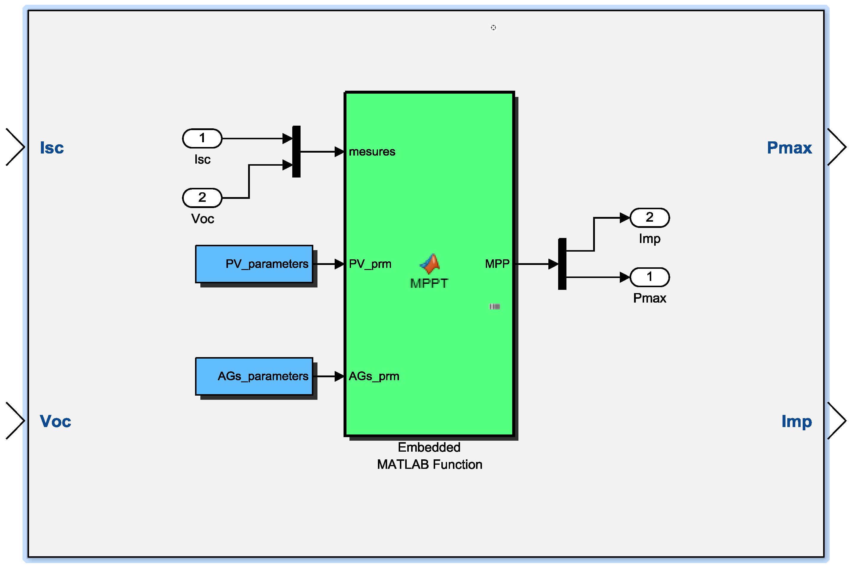
The algorithm is implemented as an embedded function on Matlab/Simulink^® using parameters of the “Conergy PowerPlus 214P” polycrystalline photovoltaic solar panel module. The inputs of the algorithm are ${\mathrm{V}}_{\mathrm{oc}}$ and ${\mathrm{I}}_{\mathrm{sc}}$ (Figure 5), so there is no need to use temperature and insolation sensors. Instead, two pilot cells are used. Temperature and insolation affect ${\mathrm{V}}_{\mathrm{oc}}$ and ${\mathrm{I}}_{\mathrm{sc}}$, respectively. By measuring these parameters, the algorithm tracks the MPP even with rapid variation of climatic conditions.

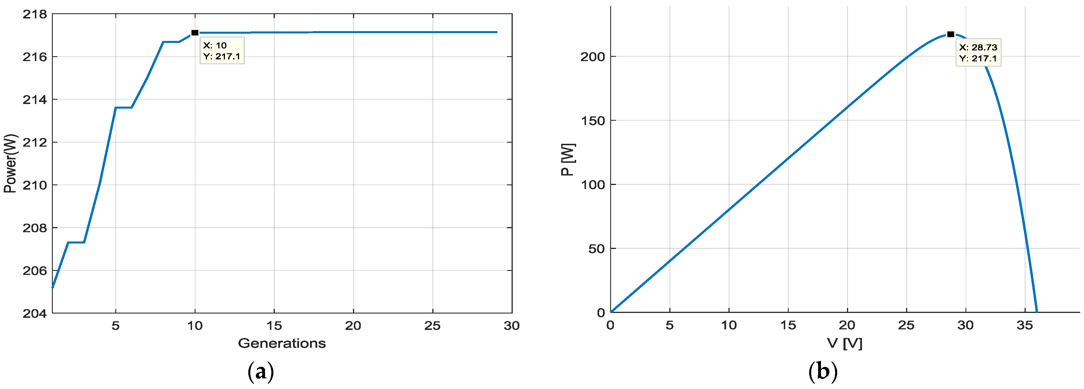
The algorithm gives the real MPP. We can see in Figure 6a the evolution of power with generations; the MPP (217.1 W) is given after 10 generations. This point is shown on Figure 6b and it is the real MPP.

The algorithm is tested by changing the matrix dimensions (Number of individuals N_ind and bits number S), with Selection rate: T_sel = 0.8; Crossover rate: T_rcm = 0.8; Mutation Probability: P_m = 0.01.

4.1. Changing Number of Individuals

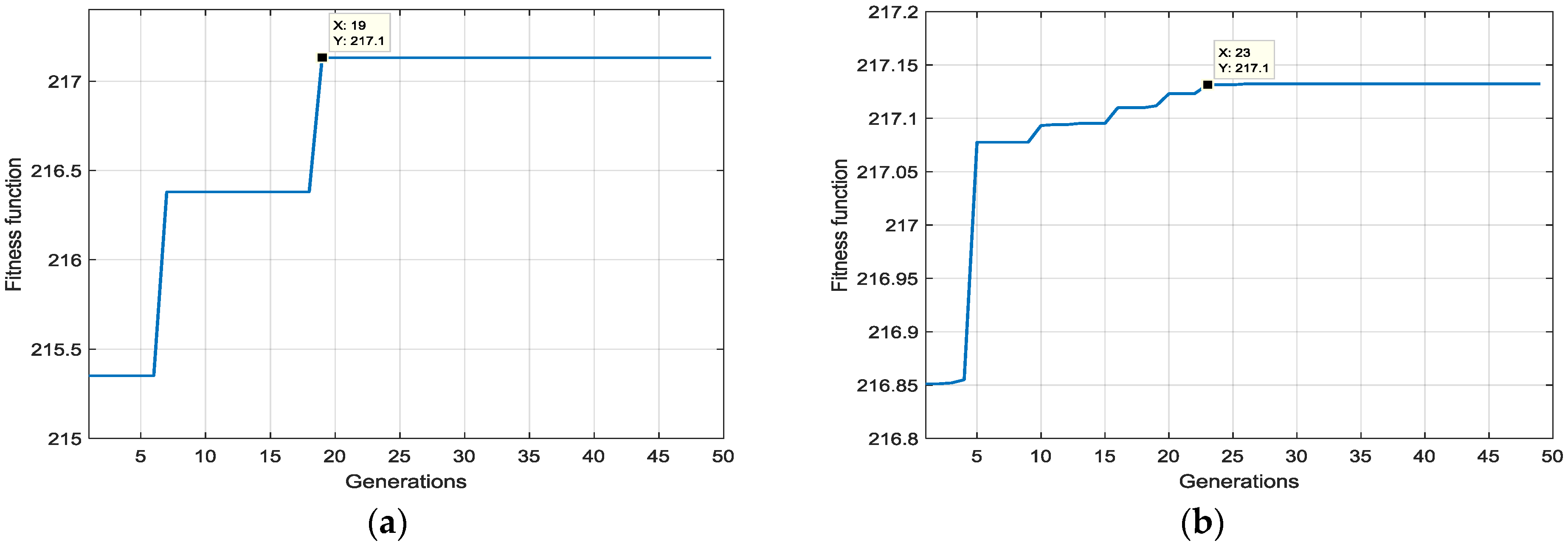
Figure 7a,b shows fitness function evolution for each generation using 30 individuals and 10 individuals, respectively. With a population of 30 individuals, the MPP (217.1 W) is achieved by the 25th generation, while it appears in the 33rd generation when using 10 individuals.

4.2. Changing Bits Number (Accuracy)

Figure 8a,b shows fitness function evolution for each generation using 8 bits and 32 bits, respectively. With a larger bits number, we get greater accuracy but slower convergence. However, the variation of power obtained with a small bits number is more important.

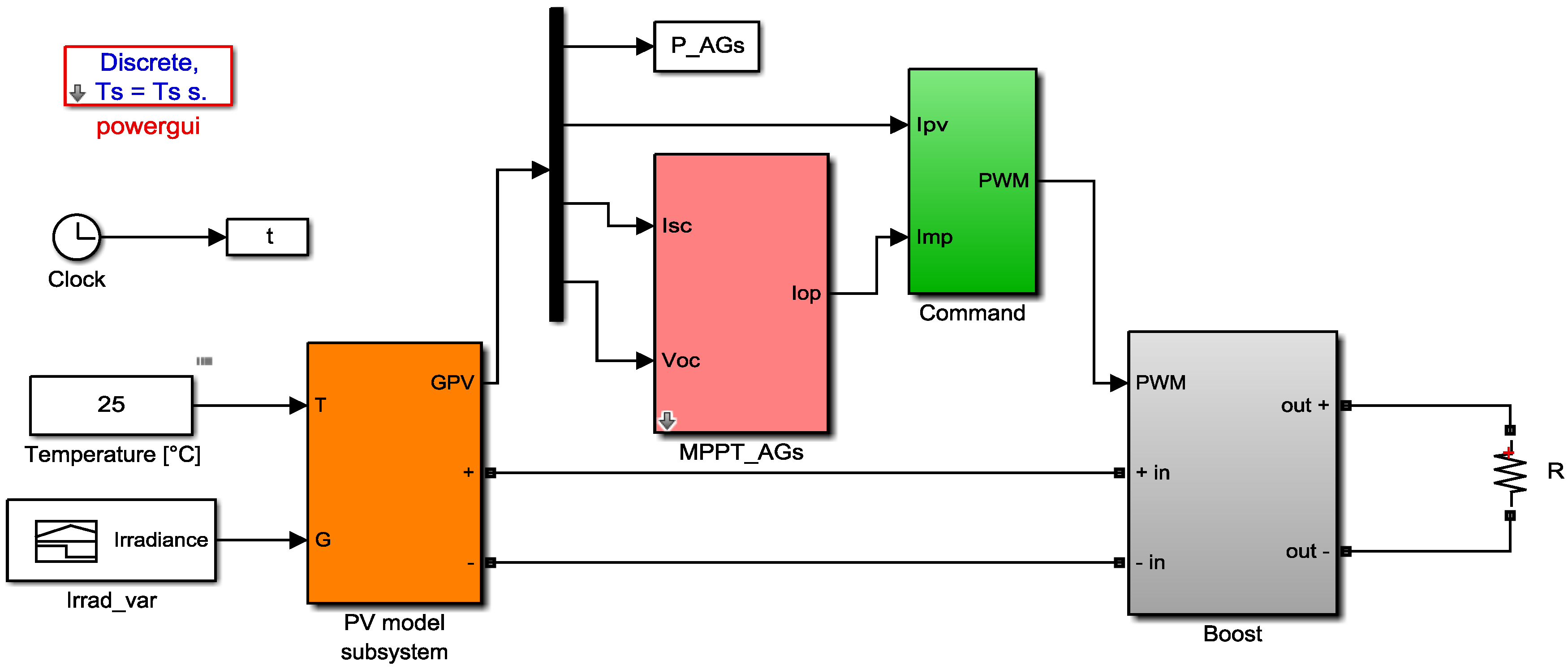
5. Simulation Tests

To test the algorithm under climatic variation, the Simulink block of GAs-based MPPT is inserted in the PV system (Figure 9).

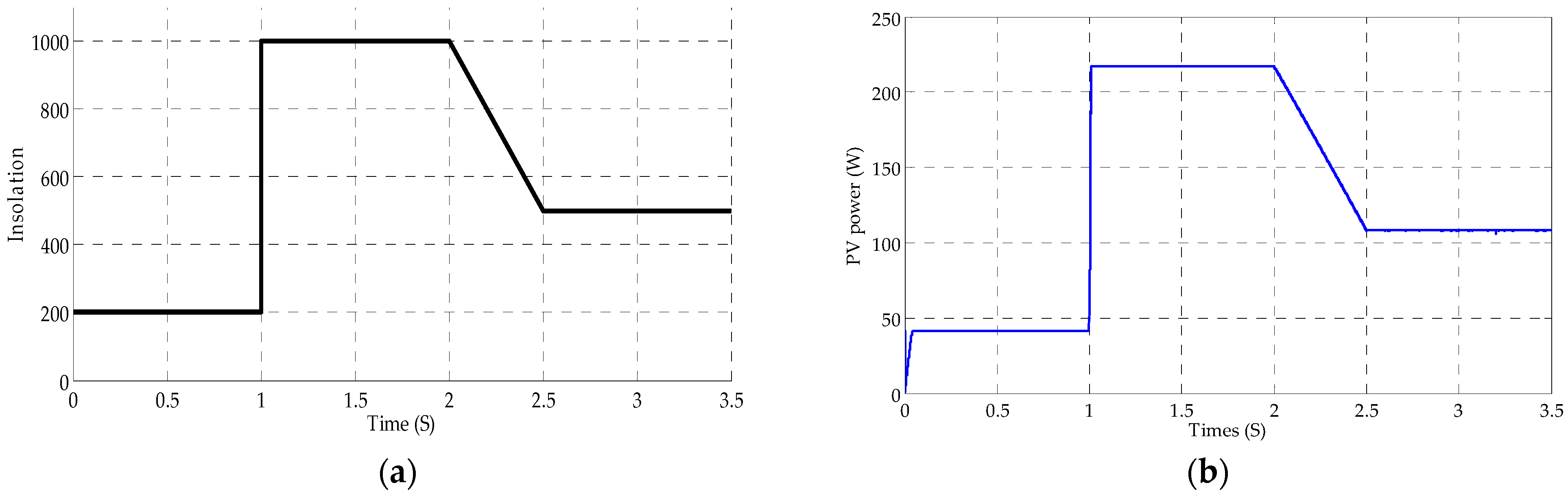
An irradiation model is applied (Figure 10a) to the PV generator. Figure 10b shows the PV power evolution using GAs-based MPPT, one can observe the rapid response of the algorithm to the variation in insolation.

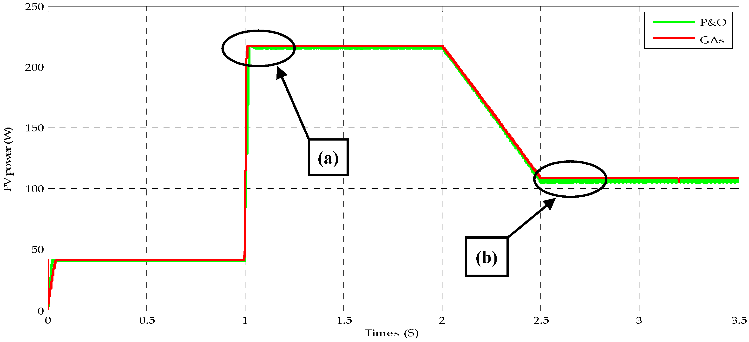
Figure 11 shows PV output power evolution using GAs (red curve) and PO (green curve). Zooming in on the graph exposes the difference between the two methods (Figure 12).

The Figure 12a illustrates the response time of the two controllers. One can notice that the GAs-based MPPT ensures better rapidity than the PO technique: 1.010 s with the proposed method compared to 1.025 s with PO. The observable power oscillations (Figure 12b) are much greater with the PO method. Oscillations are about 3% of the power with PO and less than 0.1% with the proposed algorithm, so less power is lost and more stability is guaranteed.

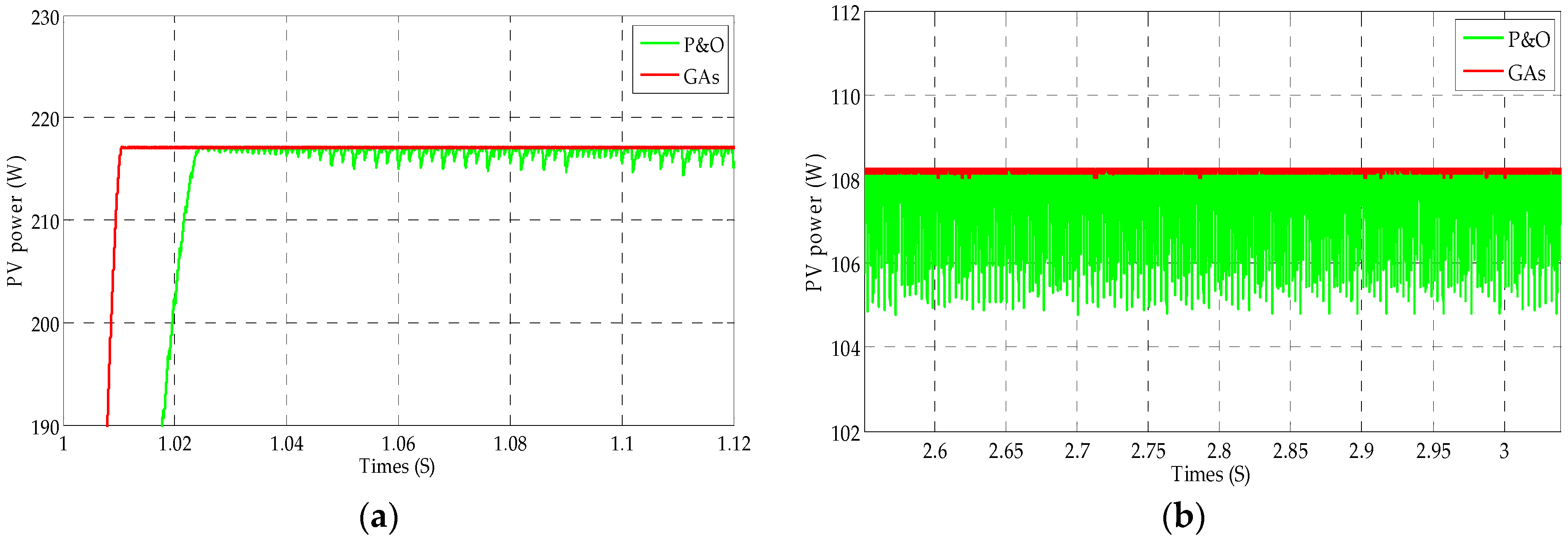
Figure 13 shows PV output power evolution with time and variable insolation by using GAs-based MPPT (red curve) and IC controller (blue curve) with duty increment ∆D = 0.02. The two methods track the MPP but the rapidity of the proposed method is clearly better than the IC method (Figure 14a). Also, the power oscillation around the MPP is minimized (Figure 14b).

If the ∆D value is increased, tracking will be faster but the oscillations will be more sizeable.

6. Experimental Tests

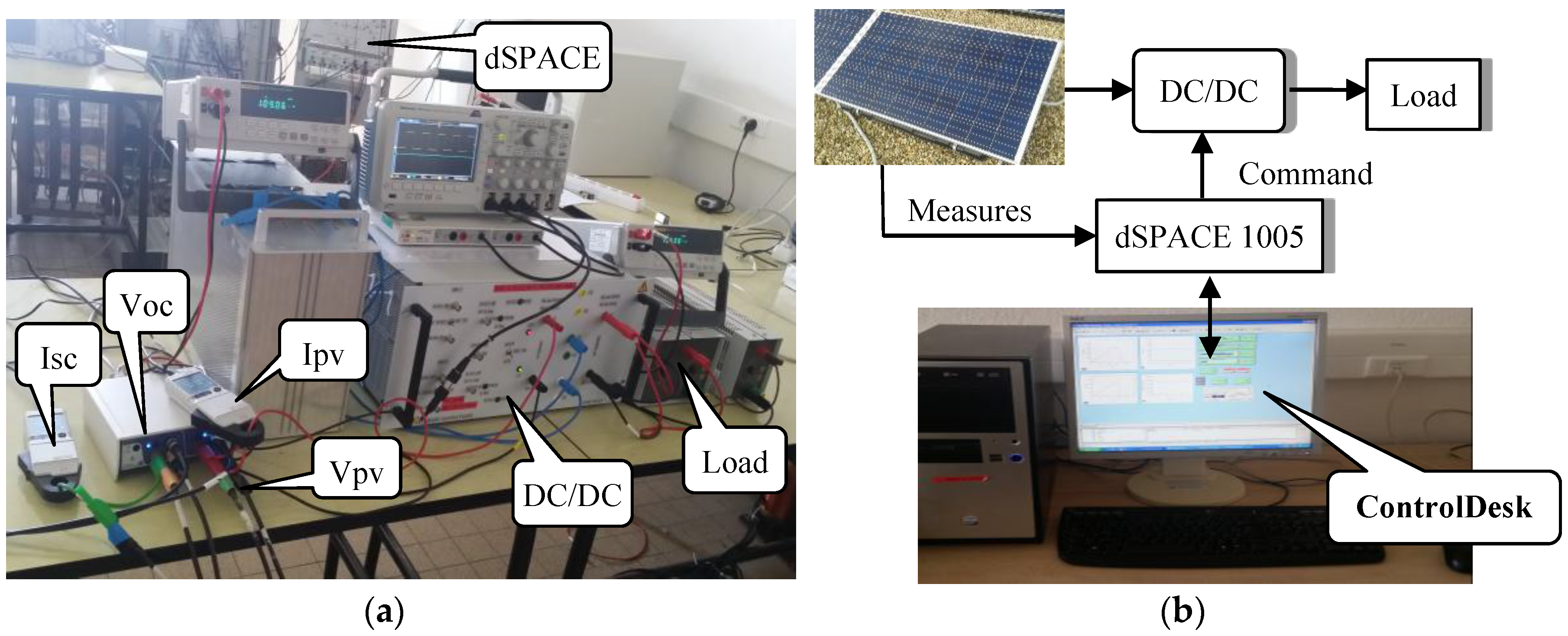
Experimental work was performed in the LIAS laboratory (Laboratoire d’Informatique et d’Automatique pour les Systèmes) of Poitiers University, France (Figure 15a). GAs-based, PO, and IC MPPT algorithms are implemented on a real-time interface (dSPACE1005) [21] which is inserted in a real PV system with 3 panels (Figure 15b).

Differential probes (PR30) are used to measure the PV voltage and ${\mathrm{V}}_{\mathrm{oc}}$ (bandwidth: 20 MHz, accuracy: ±2%, maximum voltage: 1 KVDC, input impedance: 4 MΩ//2.5 pF), and current clamps to measure the PV current and ${\mathrm{I}}_{\mathrm{sc}}$ (bandwidth > 100 kHz, current range: 1–30 A, accuracy: ±1%).

All data and results (${\mathrm{I}}_{\mathrm{pv}},{\mathrm{V}}_{\mathrm{pv}}$, PV power, duty cycle …) are collected in real-time from dSPACE1005 using the ControlDesk^® package. The step of measurements is $5\times {10}^{-5}$ s so we get continuous experimental curves.

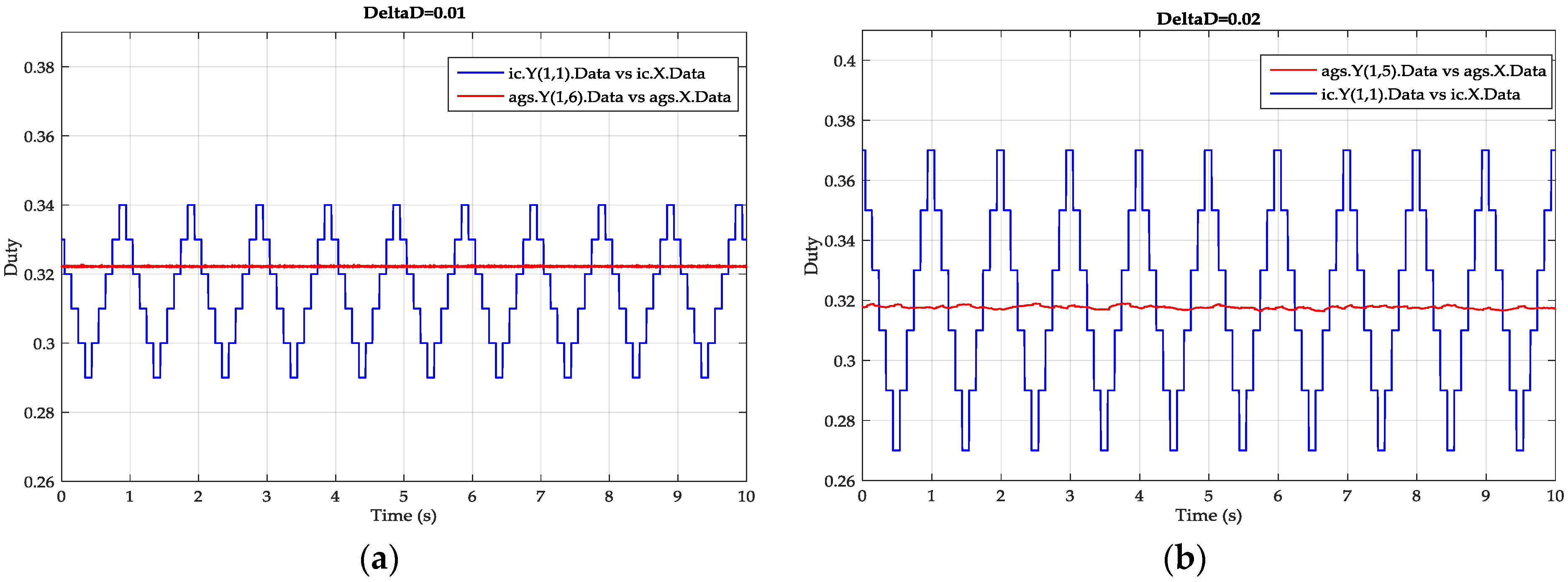
6.1. Comparing GAs and IC

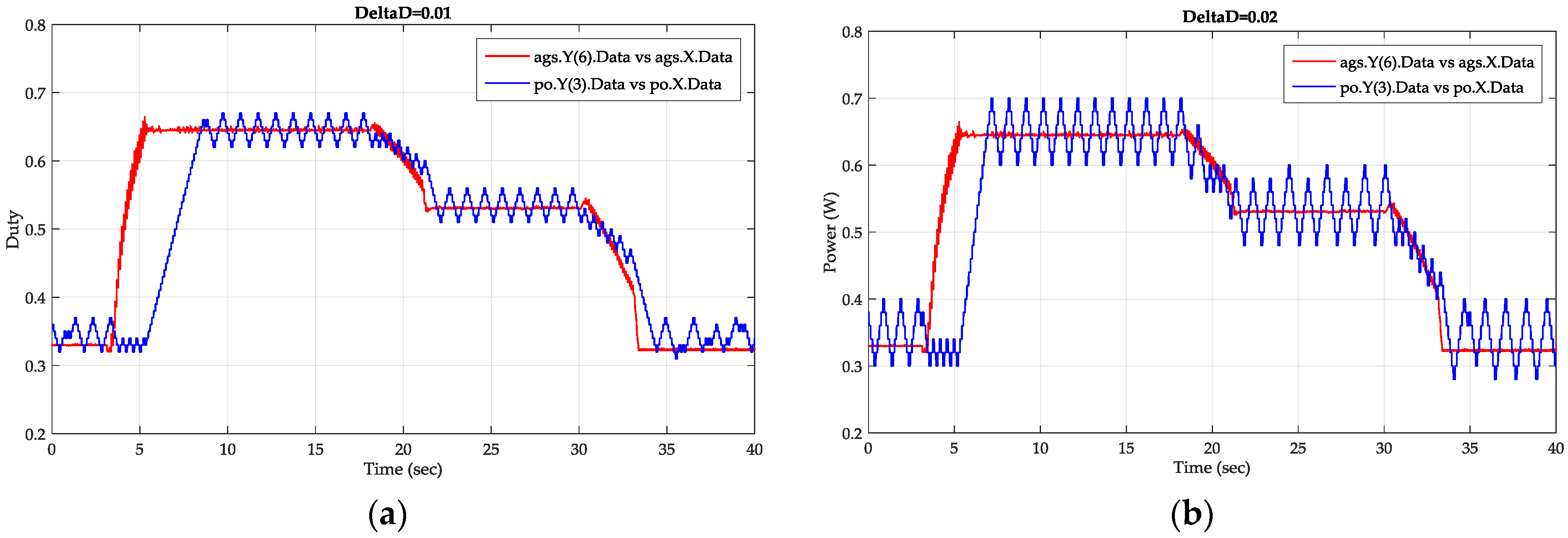
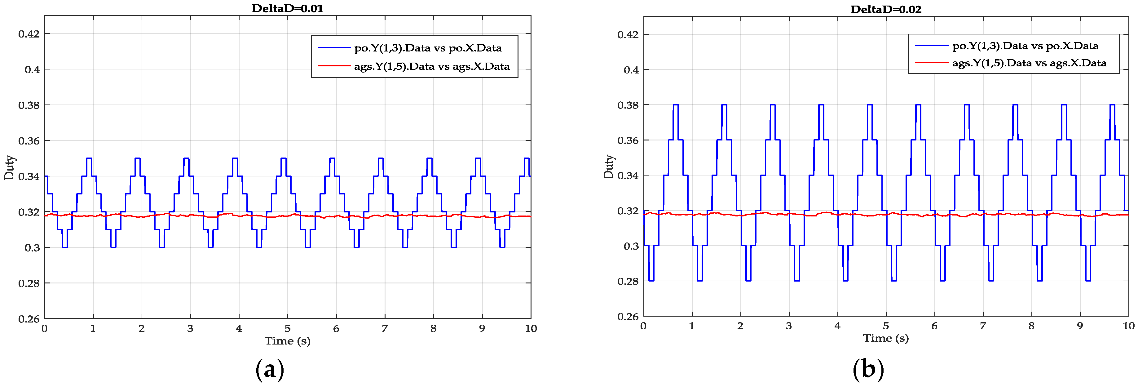
Experimental duty cycle evolution with the proposed algorithm and IC algorithm is shown on Figure 16, with duty increment $\Delta \mathrm{D}=0.01$ (Figure 16a) and $\Delta \mathrm{D}=0.02$ (Figure 16b) of the IC algorithm.

It is clear that the duty cycle is more stable with the proposed algorithm. With the IC algorithm the duty cycle oscillates between 0.29 and 0.34 with $\Delta \mathrm{D}=0.01$, and between 0.27 and 0.37 with $\Delta \mathrm{D}=0.02$, which causes oscillation of power while with the proposed method the duty cycle is practically constant. One can say that with GAs, the duty cycle is constant and the PV output power is stable and thus the problem of power oscillation is solved.

Oscillation of duty in the IC method is less important with $\Delta \mathrm{D}=0.01$ than with $\Delta \mathrm{D}=0.02$ but this will decrease the response time (see next section). Kivimäki et al. [22,23] discussed perturbation frequency (limited by the combined energy conversion system settling time) and perturbation step size (must be high enough to differentiate system response from that caused by irradiation variation). With the proposed algorithm, the problem of limitation in step size is not present because the MPP is not tracked point by point (as it is with the IC and PO methods).

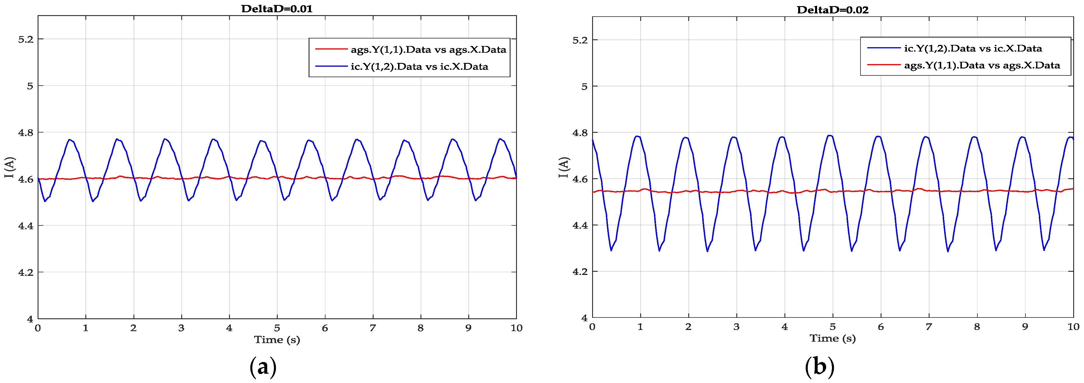
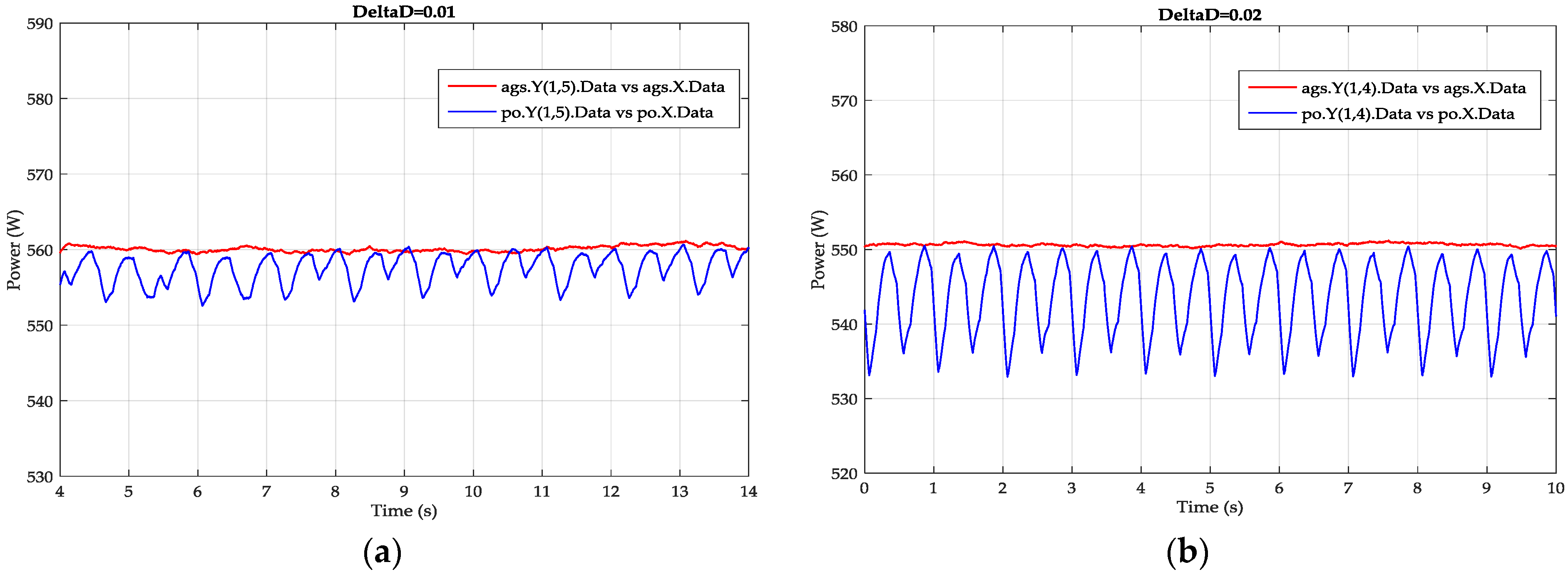
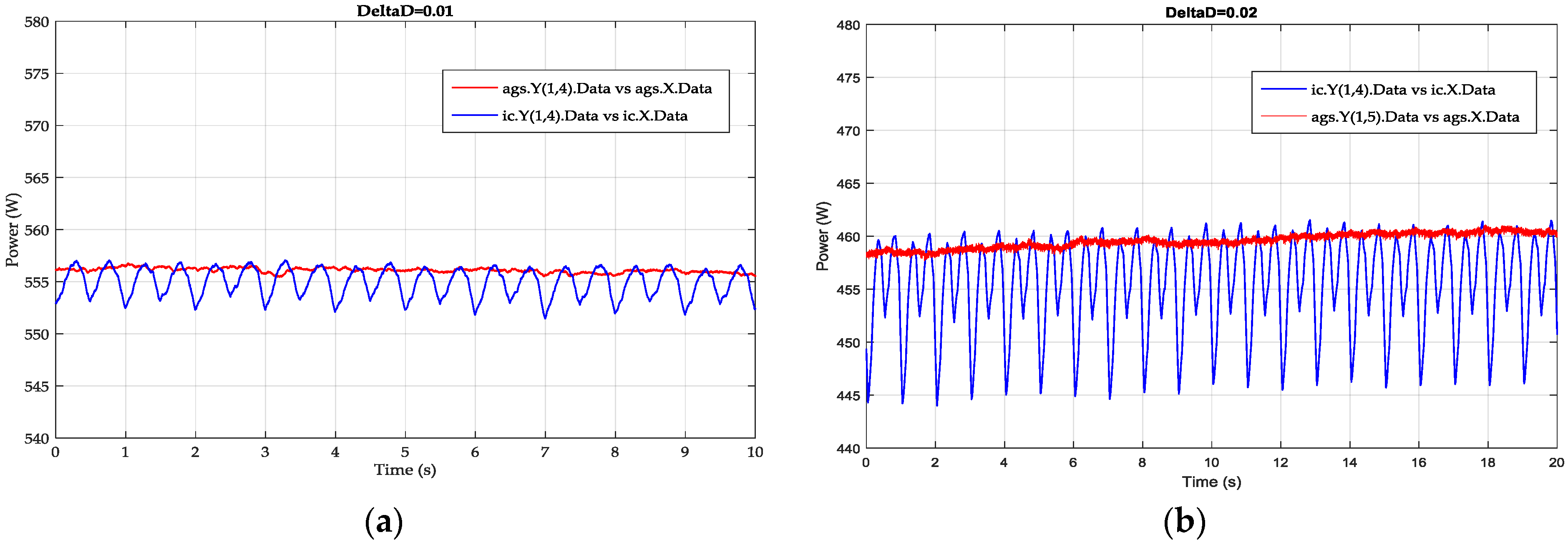
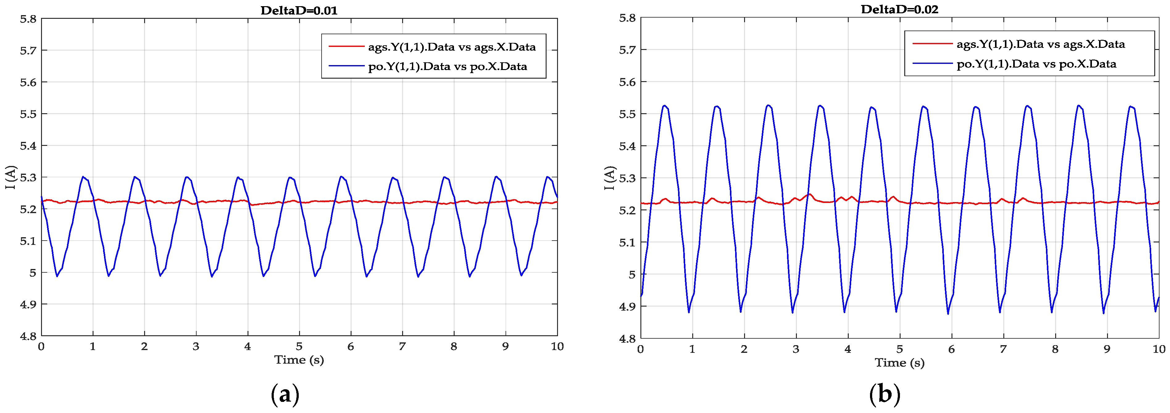
The stability of the duty cycle results in stability of the PV current (Figure 17) and PV power (Figure 18), so we get a PV system more stable with the proposed algorithm, about 1.1% and 3.3% of power is saved, respectively, with $\Delta \mathrm{D}=0.01$ and $\Delta \mathrm{D}=0.02$.

6.2. Comparing GAs and PO

Figure 19 shows the experimental evolution of the duty cycle with both GAs-based MPPT and the PO algorithm, with duty increment $\Delta \mathrm{D}=0.01$ (Figure 19a) and $\Delta \mathrm{D}=0.02$ (Figure 19b) of the PO algorithm. Even if the climatic conditions are stable (conditions of experimental tests) the duty oscillates, while with the proposed controller the duty cycle is stable. This stability can also be seen in the PV current (Figure 20).

The evolution of the output PV power with the two methods is shown in Figure 21. The goal of obtaining a stable power is guaranteed with the proposed algorithm and about 1.3% and 3.2% power is saved, respectively, with $\Delta \mathrm{D}=0.01$ and $\Delta \mathrm{D}=0.02$.

The experimental results confirm the simulated results and prove the stability of GAs-based MPPT compared to the conventional methods. One can see clearly less variation of power with the proposed algorithm, and therefore better efficiency. This is due to a stable reference (optimal current), whereas oscillations result from the variation in the duty cycle when using the PO and IC methods even under constant climatic conditions. We can further reduce ΔD but the tracking of MPP becomes slow.

7. Experimental Tests with PV Emulator

A PV emulator realized by Kadri et al. [24,25] in the LIAS laboratory (Figure 22b) allowed us to define an irradiance profile changing (Figure 22a). It is based on a programmable DC power supply GEN300-11 (voltage range: 0–300 V, current range: 0–11 A, maximum output power: 3300 W) so it can replace the three PV panels used.

The PV emulator is inserted in the PV system instead of the PV panels, so we can test the tracking of the MPP by the three methods with variable insolation.

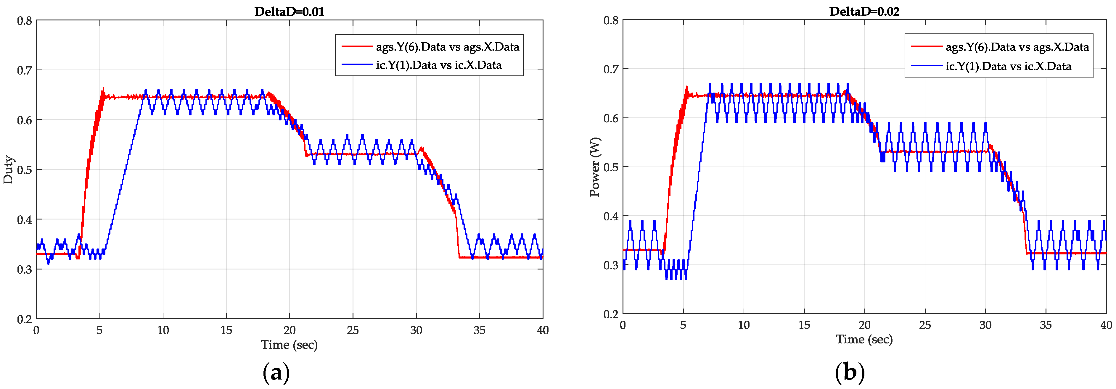
7.1. Comparing GAs and IC

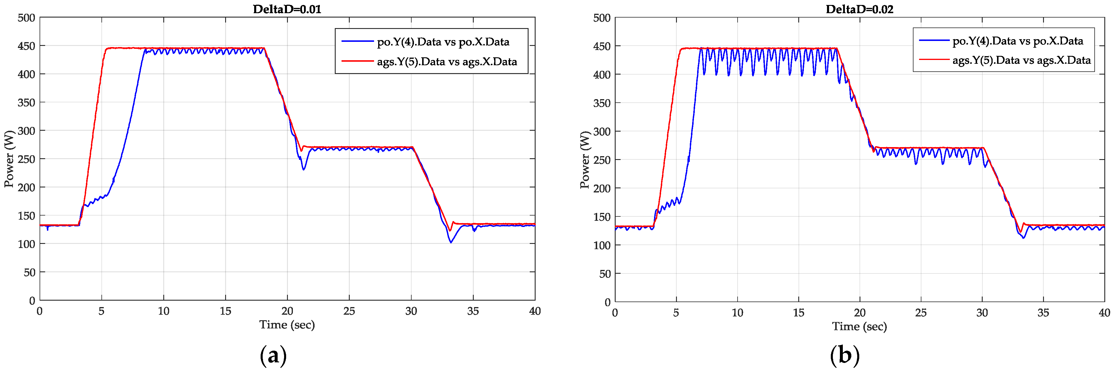
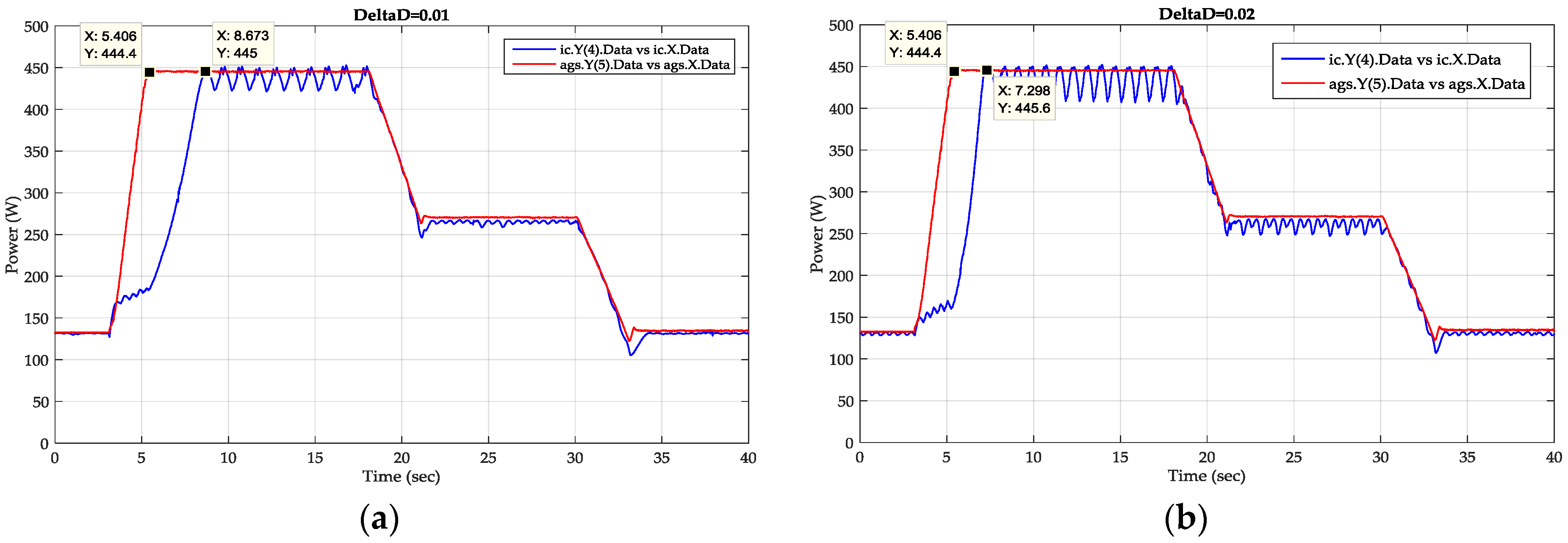
With the insolation profile defined previously, the next figures show the evolution duty cycle (Figure 23) and PV power (Figure 24) with both GAs-based MPPT and the IC method.

The power evolution with the proposed method (red curve) is clearly more stable and faster than with the IC method (blue curve).

Less oscillations of the duty cycle and power are obtained with $\Delta \mathrm{D}=0.01$ but the MPP is tracked faster with $\Delta \mathrm{D}=0.02$. For example, the maximum of insolation is given at $\mathrm{t}=5.0\mathrm{s}$ (Figure 22a). With the proposed algorithm the MPP is tracked at $\mathrm{t}=5.4\mathrm{s}$, while with IC method the MPP is obtained at $\mathrm{t}=8.7\mathrm{s}$ and $\mathrm{t}=7.3\mathrm{s}$, with $\Delta \mathrm{D}=0.01$ and $\Delta \mathrm{D}=0.02,$ respectively.

Therefore, the GAs method rapidly tracks the MPP (red curve) and solves the problem of power oscillation around it.

7.2. Comparing GAs and PO

Under the same conditions, tests are made for the PO method and the results of duty cycle and power evolution of both the GAs-based MPPT and PO methods are shown in the following figures (Figure 25 and Figure 26, respectively). Here too, the stability and rapidity of the proposed method is proven.

The problem of choosing a good duty cycle increment is not exposed with the proposed algorithm and the experimental results prove a nice stability of the controller with good rapidity.

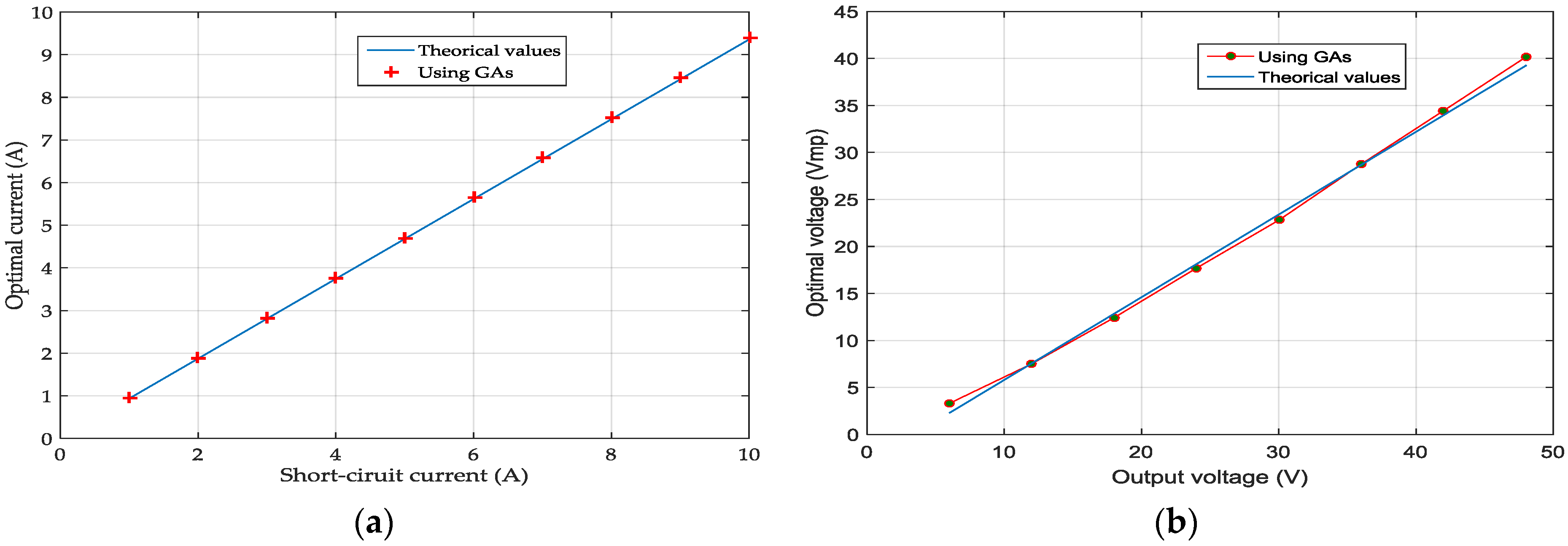
8. Verification of the Linear Method of MPPT

In order to verify Equation (2), the proposed algorithm is used to determine the optimal current Imp for different values of I_sc. The results are shown in

Table 1. Optimal current values by varying short-circuit current.

Isc (A)	1	2	3	4	5	6	7	8	9	10
Imp (A)	0.944	1.875	2.812	3.781	4.687	5.650	6.590	7.500	8.442	9.365
Mc $=\frac{{\mathbf{I}}_{\mathbf{m}\mathbf{p}}}{{\mathbf{I}}_{\mathbf{s}\mathbf{c}}}$	0.944	0.937	0.937	0.945	0.937	0.942	0.941	0.937	0.938	0.936

. The current factor can be assumed to be constant M_c $\approx 0.94$. This linearity is shown in Figure 27a.

By the same way,

Table 2. Optimal voltage values by varying open-circuit voltage.

Voc (A)	6	12	18	24	30	36	42	48
Vmp (A)	3.30	7.51	12.35	17.70	22.79	28.75	34.44	40.14
Mv $=\frac{{\mathbf{V}}_{\mathbf{m}\mathbf{p}}}{{\mathbf{V}}_{\mathbf{o}\mathbf{c}}}$	0.55	0.63	0.69	0.74	0.76	0.80	0.82	0.84

shows the optimal voltage V_mp for different values of V_oc. The voltage factor M_v is not totally constant and the real V_mp–V_oc curve is not perfectly linear (Figure 27b).

The results prove that the linear method can be used to track the MPP. Hence, the proposed algorithm can be used to rapidly calculate the current and voltage factors for any PV panel.

9. Conclusions

In this paper, a novel, simple and efficient GAs-based MPPT method is proposed.

By using the same parameters, the concordance of simulation and experimental results prove the advantage of the proposed MPPT method to ensure rapidity and stability of the output PV power. This stability is provided by maximizing a function (fitness function), whereas the conventional methods are searching for a minimum. In addition, GAs use a global search for the optimum (useful at partial shading).

The problem of PV output power oscillation around the MPP is solved. The experimental results with the IC method, using a very small step of duty cycle (ΔD = 0.01), show duty cycle oscillation between 0.31 and 0.35 which causes oscillation of power, while the duty cycle is practically constant.

The linear method is validated by our algorithm. Even better, it can be used to calculate current and voltage factors for use with the linear MPPT method.

For perspective, the GAs-based MPPT can be used to track the MPP at partial shading because the search for the optimum is performed using a population of individuals, rather than on a point-by-point basis, so it searches for the global optimum.