Abstract
Since the thermal environment of large space buildings such as stadiums can vary depending on the location of the stands, it is important to divide them into different zones and evaluate their thermal environment separately. The thermal environment can be evaluated using physical values measured with the sensors, but the occupant density of the stadium stands is high, which limits the locations available to install the sensors. As a method to resolve the limitations of installing the sensors, we propose a method to predict the thermal environment of each zone in a large space. We set six key thermal factors affecting the thermal environment in a large space to be predicted factors (indoor air temperature, mean radiant temperature, and clothing) and the fixed factors (air velocity, metabolic rate, and relative humidity). Using artificial neural network (ANN) models and the outdoor air temperature and the surface temperature of the interior walls around the stands as input data, we developed a method to predict the three thermal factors. Learning and verification datasets were established using STAR CCM+ (2016.10, Siemens PLM software, Plano, TX, USA). An analysis of each model’s prediction results showed that the prediction accuracy increased with the number of learning data points. The thermal environment evaluation process developed in this study can be used to control heating, ventilation, and air conditioning (HVAC) facilities in each zone in a large space building with sufficient learning by ANN models at the building testing or the evaluation stage.
1. Introduction
In order to maintain the indoor environment of a building pleasant and comfortable using heating, ventilation, and air conditioning (HVAC) facilities, we need to evaluate each zone’s thermal environment, which changes in real time. The thermal environment of typical residential and non-residential buildings is evaluated using one indicator, assuming that a single zone has the same thermal environment in the same space [1]. Unlike ordinary buildings, the field and wide stands are configured as one large zone in large space buildings such as indoor stadiums; uneven thermal environments can be established in the same zone. Previous studies raised issues about uneven thermal environments and excessive energy consumption in large space buildings’ occupant areas based on physical measurements and simulation methods [2,3]. Some of the most noticeable thermal environment problems with large space buildings include thermal stratification, in which a large temperature difference occurs between concentrated stands (i.e., the occupant zone) and the upper area, and uneven temperature distributions in different parts of the stands. Therefore, the thermal environment of each zone should be evaluated to properly assess the uneven thermal environments in a large space and to control HVAC.
The thermal environment felt by occupants can be evaluated by a variety of thermal environment indices that consider many different thermal factors together [4]. The thermal environment indices that comprehensively reflect the physical state of the occupants and the building [5,6] enable the control of the thermal comfort level of occupants rather than the HVAC control, which is only based on the set indoor air temperature. More importantly, the radiant temperature via a high ceiling has a significant effect on the thermal environment felt by occupants in large space buildings; therefore, it is important to evaluate the thermal environment in a way that comprehensively incorporates various thermal factors [7]. This thermal environment evaluation method requires an area to install the sensors to measure a variety of thermal factors and an additional computation process to evaluate the thermal environment.
In the application of the thermal environment evaluation method to large space buildings, a larger area is required to install sensors every time the large space is divided into more zones. Since the top priority is to ensure that people can view the field from the stands and occupant density in the stands is high, it is more difficult to install sensors effectively. Accordingly, to evaluate the thermal environment of a highly dense occupant area in real time, the sensors are placed around the stands.
Prediction methods using artificial neural networks (ANN) [8], which are machine learning methods, are widely applied in many different fields [9,10,11,12,13,14], such as the prediction of a building’s energy consumption or prediction of the weather, as ANNs do not require a process to simulate a complex system for accurate prediction [9,10,11]. If learning is done properly based on the correlation between target data and input data, the ANN has a high level of prediction performance. Antoine [12] developed a model that predicts the thermal environment of a two-story non-residential building at the next point in time using physically measured data. Furthermore, Antoine [12] implemented the HVAC system’s predicted mean vote (PMV) control into EnergyPlus and confirmed that it reduced the building’s energy consumption. To implement a real-time model-based prediction control on middle school buildings, Ferreira [13] used the radial basis function (RBF) network model and predicted the thermal environment. Castilla [14] compared the ANN and polynomial regression to predict the thermal environment and reported that the ANN has accurate higher prediction performance.
For HVAC control that considers the use and area characteristics in a large space building, it is important to predict various thermal factors in each zone and comprehensively evaluate the thermal environment. To evaluate a large space’s thermal environment using the minimum number of measuring sensors and models, we derived a method to predict the thermal environment reflecting the features of the large space. This study was conducted as follows: (1) we analyzed six thermal factors to evaluate the comprehensive thermal environment of the large space and determined the factors that required measuring and the factors that did not; (2) we built datasets to predict the thermal factors that required measuring and established a prediction method that used ANN; (3) to apply the established prediction method, we collected data from previous studies and simulations and established ANN models; and (4) we evaluated the ANN models’ accuracy according to data characteristics and model structure.
2. Deriving Prediction Process for Thermal Environment in Large Space
2.1. Setting Parameters for Predicting Thermal Envrionment
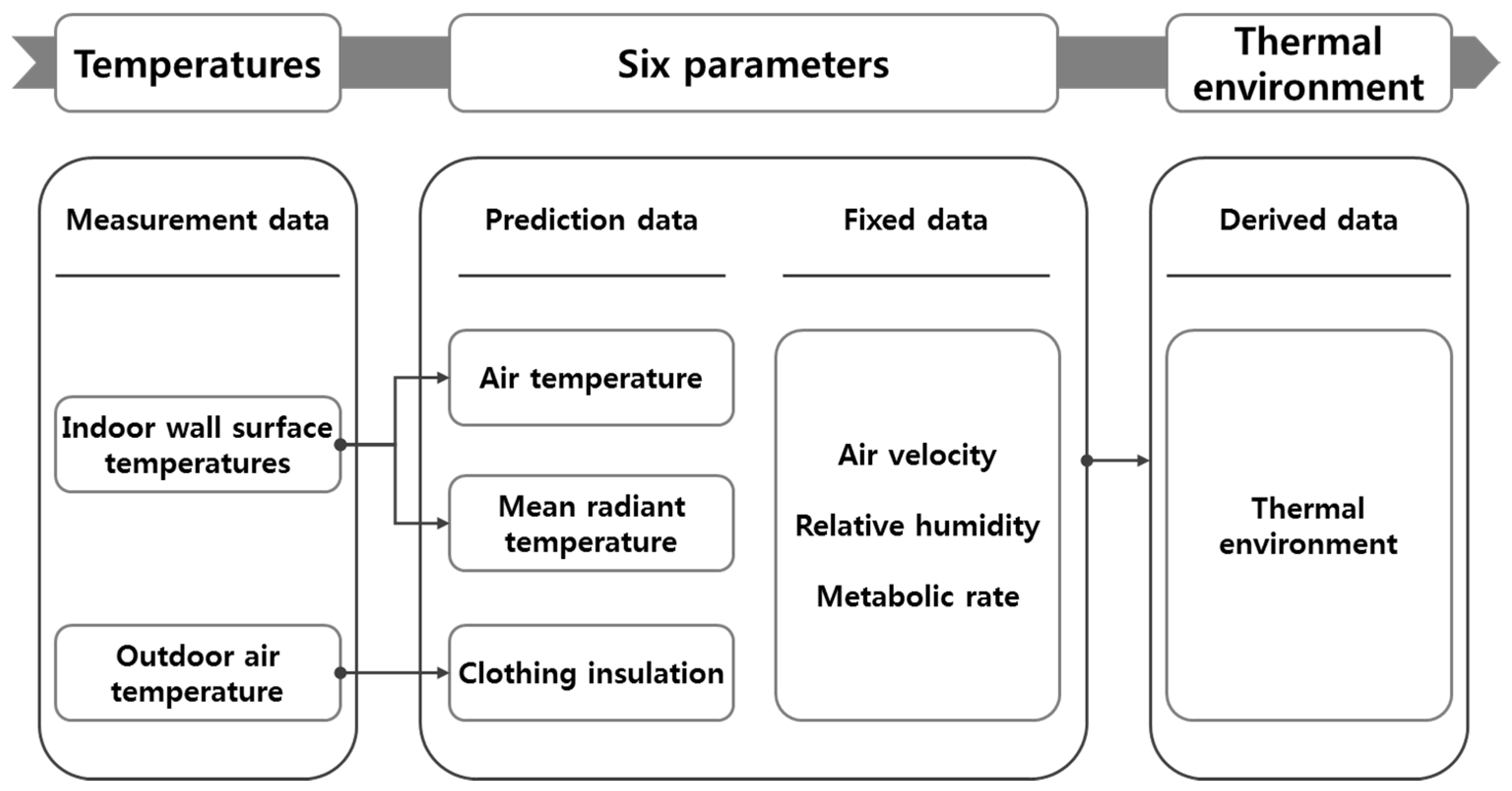
A building’s indoor thermal environment consists of physical factors and personal factors. The physical factors are objective parameters that define the thermal environment and include the indoor air temperature, the mean radiant temperature, relative humidity, and air velocity. The personal factors are subjective parameters that vary with the occupant and include clothing and the metabolic rate. These six physical and personal factors are key thermal factors to comprehensively evaluate the thermal environment and used to develop thermal environment indices such as the predicted mean vote. To predict a large space’s comprehensive thermal environment using ANN, these six thermal factors should be divided into the factors that require measuring and the fixed factors. To do this, we analyzed the characteristics of each thermal factor via a literature review considering a large space’s thermal environment characteristics and determined the factors that required measuring and those that did not. Then, we used the ANN and established datasets to predict the thermal environment.
The indoor air temperature (T) and the mean radiant temperature (MRT) are some of the thermal factors that have the largest effect on the changes in the thermal environment [7]. In a large space building, lightweight roof sheets and walls consist of materials with a high level of thermal conductivity, unlike other typical buildings, and as a result, these can lead to bigger changes in the mean radiant temperature. Thus, the mean radiant temperature and the indoor air temperature need to be measured together to predict the thermal environment. Air velocity (V) is a physical factor that affects occupants’ thermal comfort along with the indoor air temperature. The maximum airflow of the HVAC system in a large space might be too high, but the airflow is controlled at a particular value around the occupant zone. The average air velocity is usually kept at 0.5 m/s around the stands [3]. Therefore, the indoor air velocity in a large space can be controlled at around 0.5 m/s.
Relative humidity (RH) is the amount of water vapor contained in the air and varies depending on the indoor air temperature. In general, RH does not have a significant effect on thermal comfort in a moderate environment. ISO7730 [6] states that the effect of humidity on thermal comfort under a moderate temperature (26 °C or less) and a moderate metabolic rate (2 met or less) is limited. Accordingly, we assumed an RH of 50% [6,15] and set it to a fixed value. Clothing (CLO) refers to the degree of insulation by clothing, in other words, thermal resistance. While it also depends on personal attributes, it mainly varies with outdoor air temperature. In this regard, this study applied a method that predicted the clothing value based on outdoor air temperatures. The metabolic rate (MET) indicates the amount of energy consumed by an occupant in the amount of heat generated per surface area of the human body and 1.0 met is 58.15 W/m2. This study referenced a previous study on the evaluation of an indoor stadium’s thermal environment [16] and set the MET at 1.0 met.
Upon analysis of the thermal factors considering the characteristics of large space buildings based on the literature review, this study set the indoor air temperature, mean radiant temperature, and clothing as measuring (or prediction) factors to predict the thermal environment in a large space. Referencing previous studies, we set the air velocity, relative humidity, and the metabolic rate as fixed factors at 0.5 m/s, 50%, and 1.0 met, respectively.
2.2. Prediction Methodology Using ANN Models
ANNs are one of the most widely used machine learning methods to predict a particular value using large datasets. There are many different ANN models depending on how the neural networks function and the multilayer perceptron model is the most popular one [17].
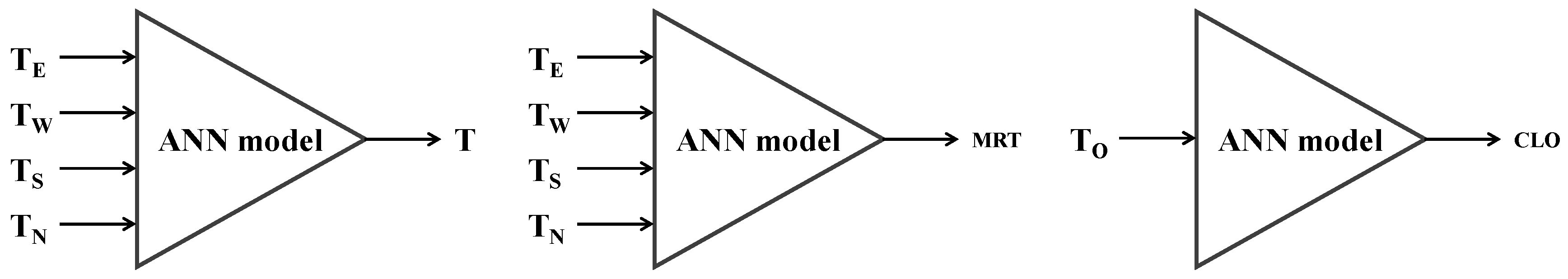
Datasets should be established to develop prediction models for three thermal factors, which require the measurements of air temperature, mean radiant temperature, and clothing. Figure 1 illustrates the output datasets of the prediction models for the three thermal factors. When the input data of a prediction model is easy to measure in a large space and is correlated to the target data to be predicted, a high level of prediction performance can be expected from an ANN model.
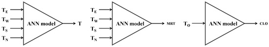
Figure 1.
Input/output data set for T (indoor air temperature), MRT (mean radiant temperature) and CLO (Clothing) estimation model.
We selected the surface temperature of the interior walls as input data to predict indoor air and mean radiant temperatures, both of which are physical factors. The indoor air temperature and the mean radiant temperature are affected by the outdoor air temperature and heat transferred to the wall due to insolation and by the HVAC system and other sources of heat inside. Interior walls come into contact with the outdoor air and their surface temperature is affected by the HVAC airflow; therefore, the interior wall surface temperature is correlated with the indoor HVAC airflow and the indoor air temperature affected by the outdoor air temperature. In addition, when calculated in simple terms, the mean radiant temperature uses the interior wall surface temperature and heat radiated from the wall. In this regard, the interior wall surface temperature can explain the changes in the indoor and outdoor environment in relation to the indoor air temperature and mean radiant temperature. If used as input data along with insolation, the outdoor air temperature, and other related factors, the interior wall surface temperature can accurately predict the indoor air temperature [18]. Since the interior wall surface temperature is affected by insolation in cardinal directions, this study set four interior wall surface temperature values: east, west, south, and north (TE, TW, TS, and TN).
Clothing as a personal factor is closely related to the outdoor air temperature. Based on a previous study on a CLO model, we selected the outdoor air temperature (TO) at 6 a.m. as input data. Unlike physical factors that are required to be predicted at suitable time intervals to control, we assumed that clothing selection of the day was determined at 6 a.m. according to the outdoor air temperature.
2.3. Thermal Environment Prediction Development Process Using ANN Models
A prediction model using ANN is developed in the order of data collection, model establishment, model learning, and model verification. At the data collection step, the data to be predicted (model output) and the data to be used for prediction (model input) are selected. Input and output datasets should be collected considering that the data characteristics and the prediction performance of a model can vary with the range of the dataset used for the model’s learning. To develop ANN models that predict indoor air temperatures, mean radiant temperatures, and clothing, data were collected from zones whose thermal environment was to be evaluated (Figure 1). We also collected data on temperature changes that fluctuate sharply in the large space under heating conditions in winter.
At the model establishment step, the type of learning method is determined by setting the ANN structure. For better model learning, the number of neural network layers, the number of neurons, the neuron transfer function, and the learning algorithm should be set at suitable levels. In general, the more hidden layers and hidden neurons exist, the more complex learning takes place, increasing the prediction performance. However, these values are not necessarily proportional to the prediction performance [19]. According to a study conducted by Carpenter [20], the number of hidden neurons should be at least one more than that of input data points. Therefore, prediction models for three thermal factors show different levels of prediction performance depending on the model structure. In this regard, based on the findings of previous studies, this study set the basic model conditions and established the data characteristics and model structure.
At the model learning step, a learning algorithm is used to learn the model structure established based on the collected data. The learning algorithm compares the target data and output data learned from the model structure and controls the weights connected between the neurons in a way that minimizes the error between the output data and target data. The rate of convergence of the error and the learning outcomes can be different depending on the type of the learning algorithm. The Levenberg–Marquardt (LM) algorithm is a good learning algorithm for most systems. To apply the LM algorithm to each of the prediction models, this study evaluated each model’s learning accuracy based on the data characteristics (the range and size of datasets) and the model structure (learning algorithm and the number of hidden neurons).
At the model verification step, data that are not used in learning (i.e., verification data) are used to evaluate the prediction performance of a learned model. By evaluating the model’s prediction results using the statistical measures of R2, RMSE (Root Mean Square Error), and MAE (Mean Absolute Error) to determine whether the errors are at similar levels, the learning data are verified.
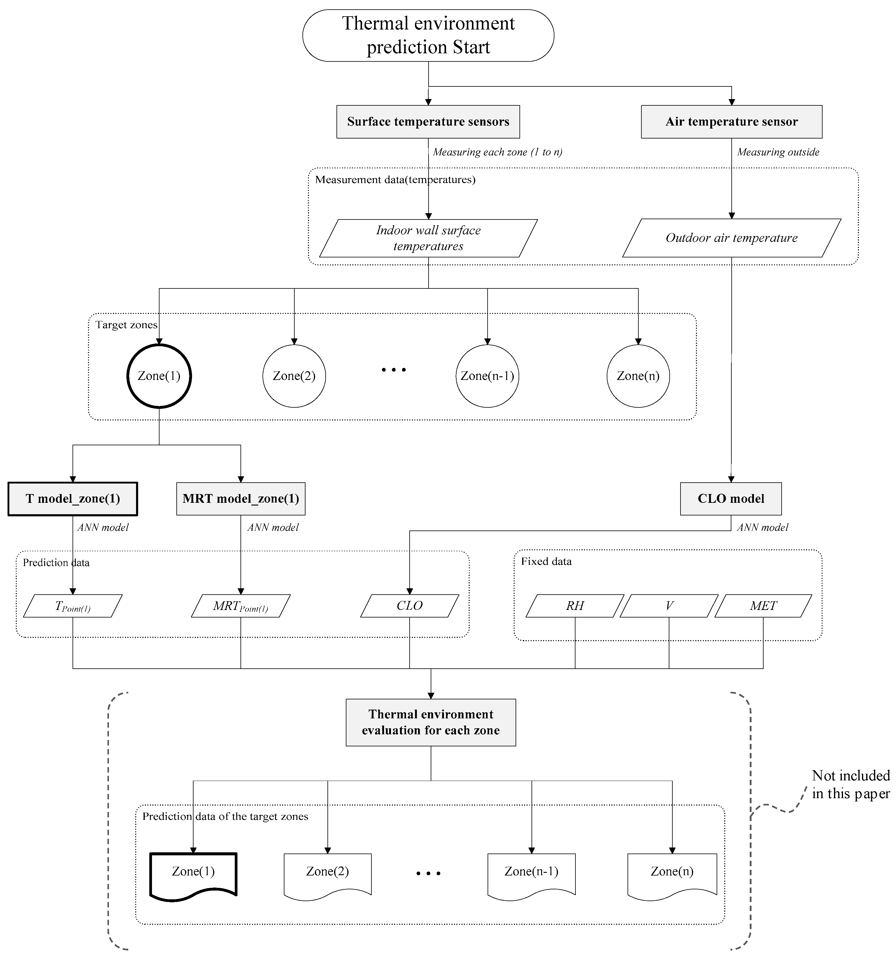
This section established a thermal environment prediction method for a large space using ANN. To predict the thermal environment, thermal factors should be predicted first from the temperature measured all around the large space in accordance with the workflow of input and output data for the model (Figure 2). The thermal environment is then derived from the six thermal factors. Data on the interior wall surface temperature and outdoor air temperature are used as input data to predict indoor air temperatures, mean radiant temperatures, and clothing.

Figure 2.
Input/output data for predicting thermal environment.
3. Development of Prediction Model for Thermal Environment in Large Space
3.1. Setting ANN Model Cases
Datasets for T and MRT models were obtained from the simulation results of the target building. Datasets for the CLO model were collected from the literature. For indoor air and mean radiant temperatures, the data that varied in each zone were used to evaluate the model accuracy according to the data characteristics. For clothing, as the data were collected from the literature based on the experimental results or computational models, the same results were used to evaluate the model accuracy based on the model structure.
To collect data in a period with the largest changes, we analyzed the lowest and highest monthly average temperatures in the last 30 years and set the target period. To consider radiant heating from the building envelope in a large space under heating conditions in winter, in which the temperature changes are most pronounced, this study selected the 28-day period that showed the largest temperature gap (8 °C) in January (the month with the lowest average temperature). Considering the available simulation resources, we set 12:00–13:00 (most insolation received) for three days (two days for learning and one day for verification) from 28 to 30 January 2015 as the data collection period. In addition, we assumed that the target building’s occupancy rate was 100% and limited effects were caused by from the changes in the body heat. We also assumed in regard to HVAC conditions that heating was started for the first time during the day. The initial indoor temperature was set at 14 °C based on a previous study by Seok [21].
We set the basic model structure as one hidden layer, the hidden layer’s transfer function logistic sigmoid, the output layer’s transfer function linear, the LM algorithm, and the number of hidden neurons one more than that of input data points (Table 1).

Table 1.
Default setting conditions for artificial neural network (ANN) model.
Based on the basic set conditions, ANN models were selected for each data characteristic and structure (Table 2 and Table 3). To collect the data patterns that appear in each zone of a large space, ANN models were divided into four cases (Cases 1 to 4) depending on the floor level (1 F to 4 F) and time interval (60 s and 300 s). Cases 5 and 6 represent the learning algorithm and the number of hidden neurons, respectively. As an example, Case 1-1 indicates a model that uses the data collected at 60-s intervals on the first floor of the building while Case 5-1 is a model that uses the LM algorithm with the number of hidden neurons one more than that of input data points. As the scaled conjugate gradient (SCG) algorithm is known to have a higher level of prediction performance than the LM algorithm when there are many weights and deviations (100 or more), it was selected as a comparison algorithm.
Table 2.
ANN models by data characteristics.
Table 3.
ANN model by model structures.
3.2. Dataset Collection: T and MRT
The dataset consists of learning data and verification data. Two different datasets were acquired for learning and verification of T and MRT models. Simulations were performed to develop T and MRT models. The interior wall surface temperature, indoor air temperature, and mean radiant temperature derived from the simulation were used as the learning data, employing CATIA (V6 R2016, Dassault systems, Vélizy-Villacoublay, France) [22] to model the target building and STAR CCM+ [23] to perform the simulation. This section describes the target building and the simulation steps after setting the prediction points in each zone for T and MRT prediction and modeling.
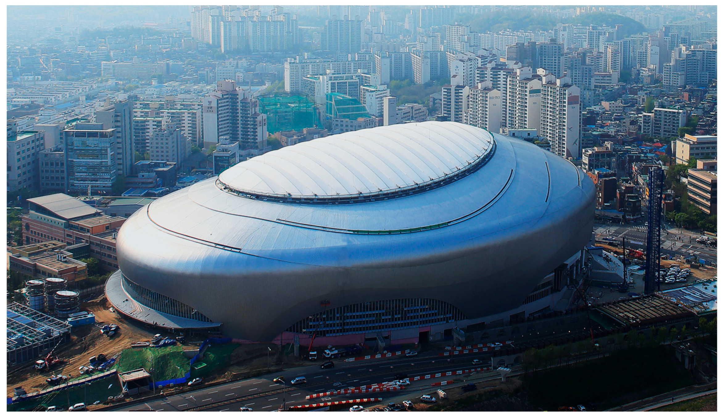
The target building is a stadium located in Guro District, Seoul. It is 67.59 m tall and has a dome at the top. It consists of two floors below ground and four floors above ground and the area is 29,120 m2 with 16,847 seats in the stands (Figure 3).

Figure 3.
Target building.
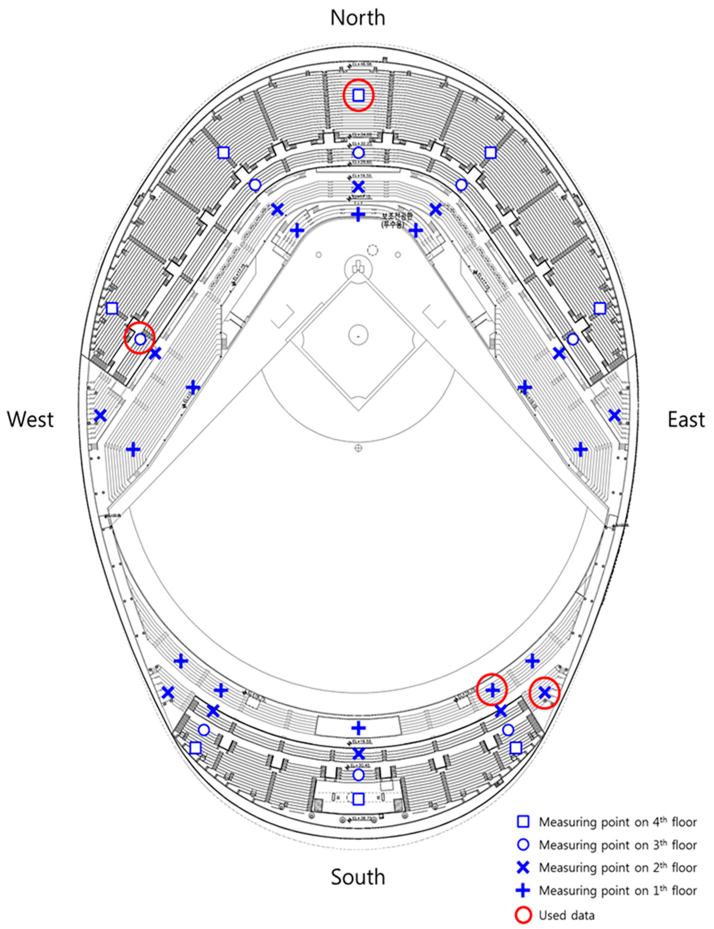
The south-north side of the target building is longer than the east-west side and the area for which the thermal environment will be predicted is where the stands are placed. The stands are placed all the way from the first to the fourth floors to the north of the infield and south of the outfield. The thermal environment data collection in each zone was based on the cardinal directions, floor level (height), envelop materials, and the layout of air inlets. Figure 4 demonstrates the data collection points.
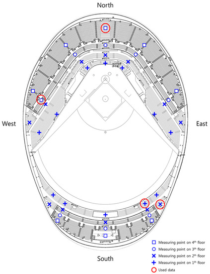
Figure 4.
Measuring points for data collection on each floor.
The plan of the actual building was simplified to model the building more efficiently. As the stands were used for the analysis of the thermal environment, only the height of the stands was considered; the chairs in the stands and other indoor structures were not included in the analysis [24]. Simulation boundary conditions were categorized into air inlets, air outlets, physical properties of a structure, and human body heat conditions. Since the HVAC plan of a large space building is extremely complicated, air inlets and outlets on the same floor were simplified and combined into 11 groups. Based on a reference facility design, the flow rate and the temperature at the air inlet were set at 4.6 m/s and 31 °C, respectively. The physical properties of structures such as glass, concrete, galvanized sheets, membranes, and outdoor conditions were set depending on the location of the building. For human body heat, the human skin temperature was set at 34 °C in the stands according to Chen [25] considering that it ranges 28 to 36 °C when it is cold and is approximately 36 °C when it is hot.
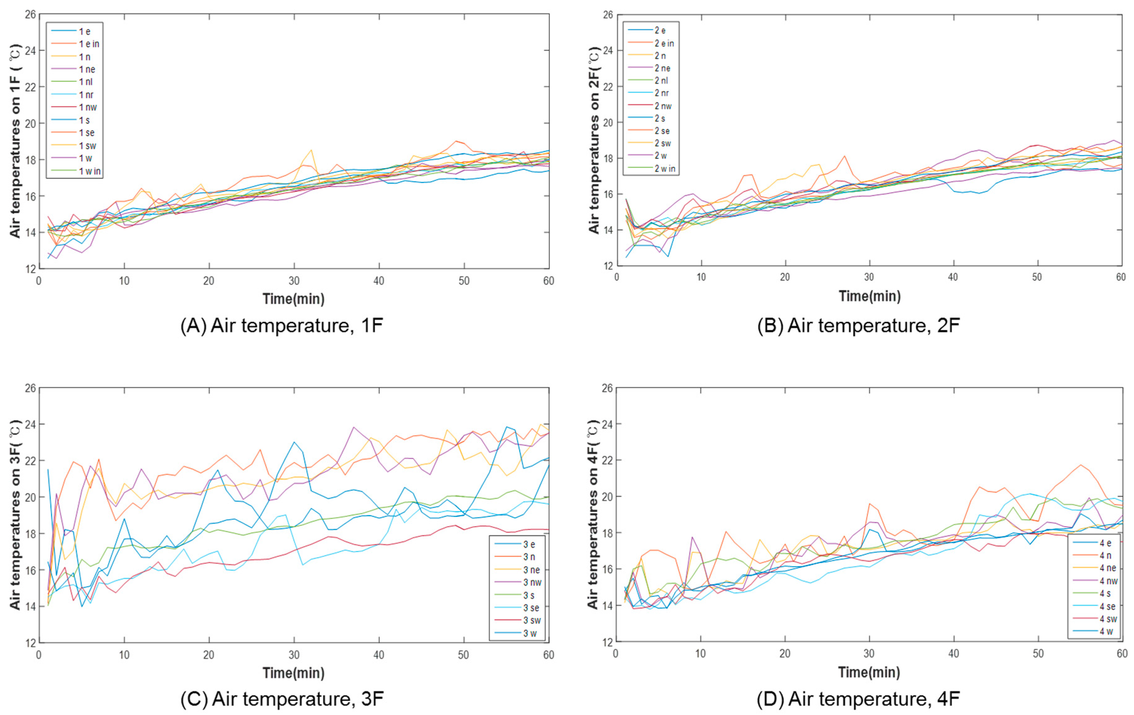
The simulation was performed for the data collection purposes (i.e., learning and verification data). The simulation program can produce different results depending on the simulation conditions set by the user. Therefore, we analyzed the trends in the data reported in previous studies [14,26] and determined the learning dataset suitable to evaluate the model accuracy. The simulation results for the interior wall surface temperature, indoor air temperature, and mean radiant temperature varied with the cardinal direction and floor level. The indoor air temperature was affected more strongly by the floor level than the cardinal direction; the indoor air temperature on each floor is depicted in Figure 5. Since the heating temperature of 31 °C lasted about an hour at the initial temperature of 14 °C, we were able to determine the overall tendency even though all values increased, time intervals for the collected data were very short, and the values were not stable.
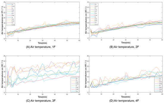
Figure 5.
Distribution of air temperature on each floor.
The temperature ranged from 12 °C to 19 °C on the first and second floors depending on the cardinal direction and as the dataset size gradually increased. The temperature ranged from 13 °C to 24 °C on the third floor and from 13 °C to 20 °C on the fourth floor. On the third floor, in particular, the temperature varied significantly with the cardinal direction after one hour and showed larger changes than on the first, second, and fourth floors. The third floor was affected by air buoyancy from the height and hot air coming from the first, second, and fourth floors. The fourth floor showed smaller changes than the third floor because the fourth floor was in contact with the roof, which is affected by the outdoor air temperature.
Cases 1 to 4 were selected based on the point of each floor that showed the largest changes in the indoor air temperature on 28 January (Table 2) and further specified into more cases such as Case 1-1 or Case 1-2 based on the time intervals of data collection (60 s, 300 s). Within the data collection period of 28–30 January 2015, we used the data collected on 28 and 29 January for learning and on 30 January for verification. Table 4 shows the range of the interior wall surface, indoor air, and mean radiant temperature values for the points selected (Figure 4).
Table 4.
Maximum and minimum range of dataset for T and MRT prediction models.
3.3. Dataset Collection: CLO
The CLO model was developed using the 6 am outdoor air temperature data from the ASHRAE RP-884 public database [27]. The data used in this study included the Ottawa Canada-winter, Grand Rapids MI-winter, and Peshawar Pakistan-winter and summer data [27]. All these locations are mid-latitude regions with a climate similar to that of Korea. The range of outdoor air temperatures in the learning dataset was set in a way that fully included the temperature changes during the season. A total of 64 datasets were collected; 57 of them were used for learning and seven for verification. Table 5 presents the range of data used in the CLO model.
Table 5.
Maximum and minimum range of dataset for CLO prediction model.
3.4. Deriving Thermal Environment Prediction Process in Large Space
ANN prediction models were divided into the indoor air temperature prediction model (T model), the mean radiant temperature prediction model (MRT model), and the clothing model (CLO model). Interior wall surface temperature data were input to the T and MRT models to predict indoor air and mean radiant temperatures; the outdoor air temperature data were input to the CLO model to predict clothing. The predicted values on indoor air temperatures, mean radiant temperatures, and clothing, and the set values on air velocity, relative humidity, and MET allowed the large building’s thermal environment to be evaluated comprehensively.
Occupants in a large space feel different thermal environments depending on their location and surroundings. Therefore, a large space should be divided into multiple zones to measure its thermal environment and control HVAC. The thermal environment prediction process that represents this idea is shown in Figure 6. Note that this study aims to predict three parameters (i.e., T, MRT, and CLO) in a large space, and the thermal environment evaluation was not included in this paper. The applicability of the thermal environment evaluation for an actual building is discussed in Section 4.2 and conclusion. For the thermal environment prediction in each zone, the prediction model was expanded into multiple models to predict indoor air and mean radiant temperatures that varied in each zone. Clothing was predicted in all zones with one value. The measured factors, which served as variables for thermal environment prediction in each zone, were indoor air temperature and mean radiant temperature. Using MATLAB’s neural network tool (2016, The MathWorks, Natick, MA, USA), we designed the ANN models in such a way to learn each case that predicted indoor air temperatures, mean radiant temperatures, and clothing.

Figure 6.
Thermal environment prediction process in a large space.
4. Evaluation of Thermal Environment Prediction Performance
4.1. Evaluation of ANN Model According to the Data Characteristics
The accuracy of T and MRT models was evaluated according to their data characteristics. For ANN model cases selected in Section 3.1, we developed T and MRT models using the learning datasets of indoor air and mean radiant temperatures in Section 3.2 (Table 2 and Table 4). In this section, we set the number of neurons (4-5-1: number of input neurons, number of hidden neurons, and number of output neurons), the learning algorithm, and the transfer function at basic conditions for the model structure (Table 1) and evaluated the model accuracy depending on the floor level and the number of data points. Table 6 presents the accuracy of each prediction model case evaluated using the statistical measures of Coefficient of determination (R2), Root Mean Square Error (RMSE), and Mean Absolute Error (MAE). R2 is obtained from the linear regression and indicates how well the variation of the data can be explained. It has a value between 0 and 1, and the closer the value is to 1, the higher the correlation between the two values. RMSE represents the accuracy of the model as a measure of how far the predicted value is from the target value, and MAE is the average of the absolute error between the predicted value and the target value. The prediction performance is higher as the values are close to 0.
Table 6.
Accuracy of T and MRT prediction models according to the data characteristic.
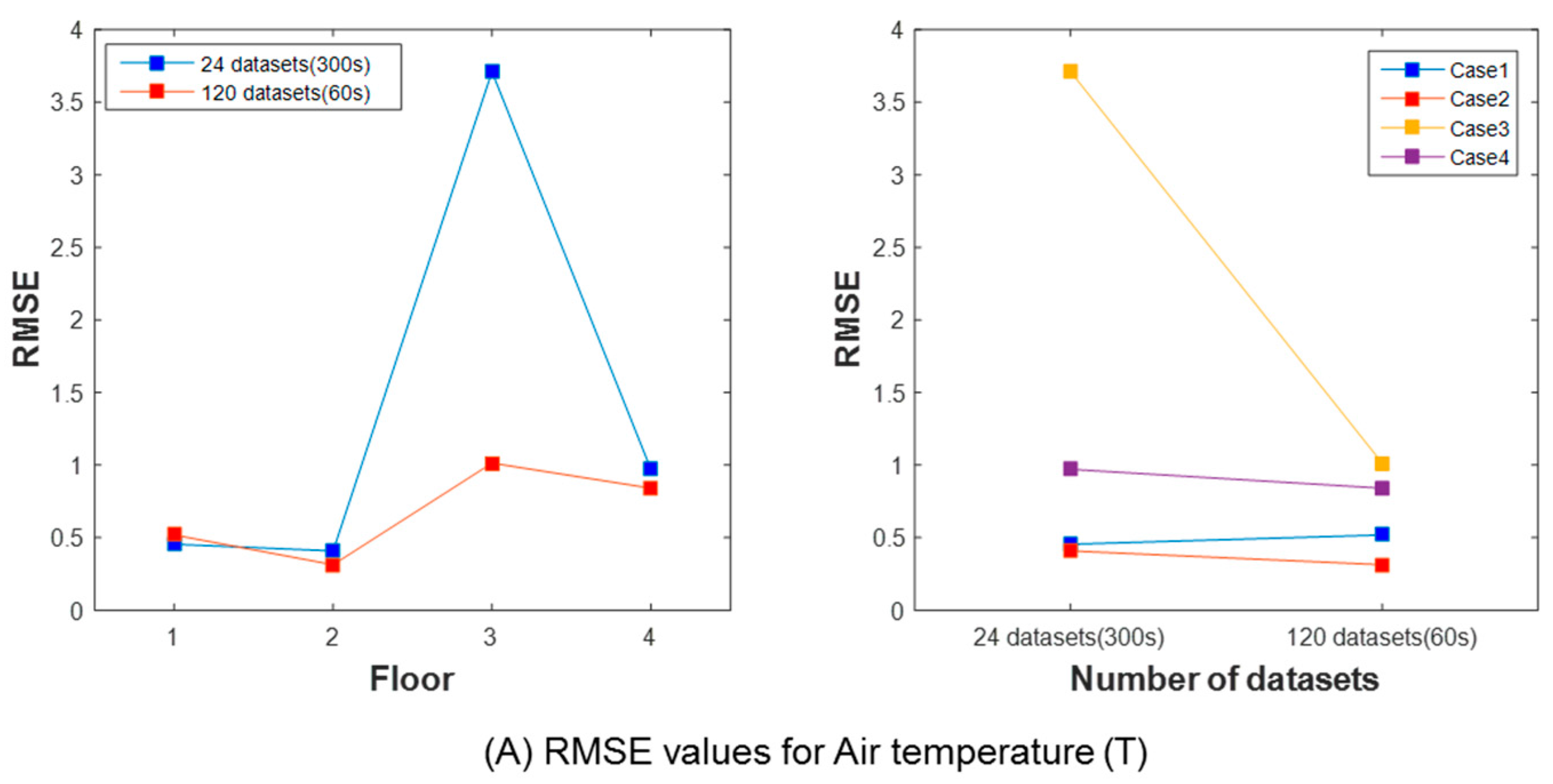
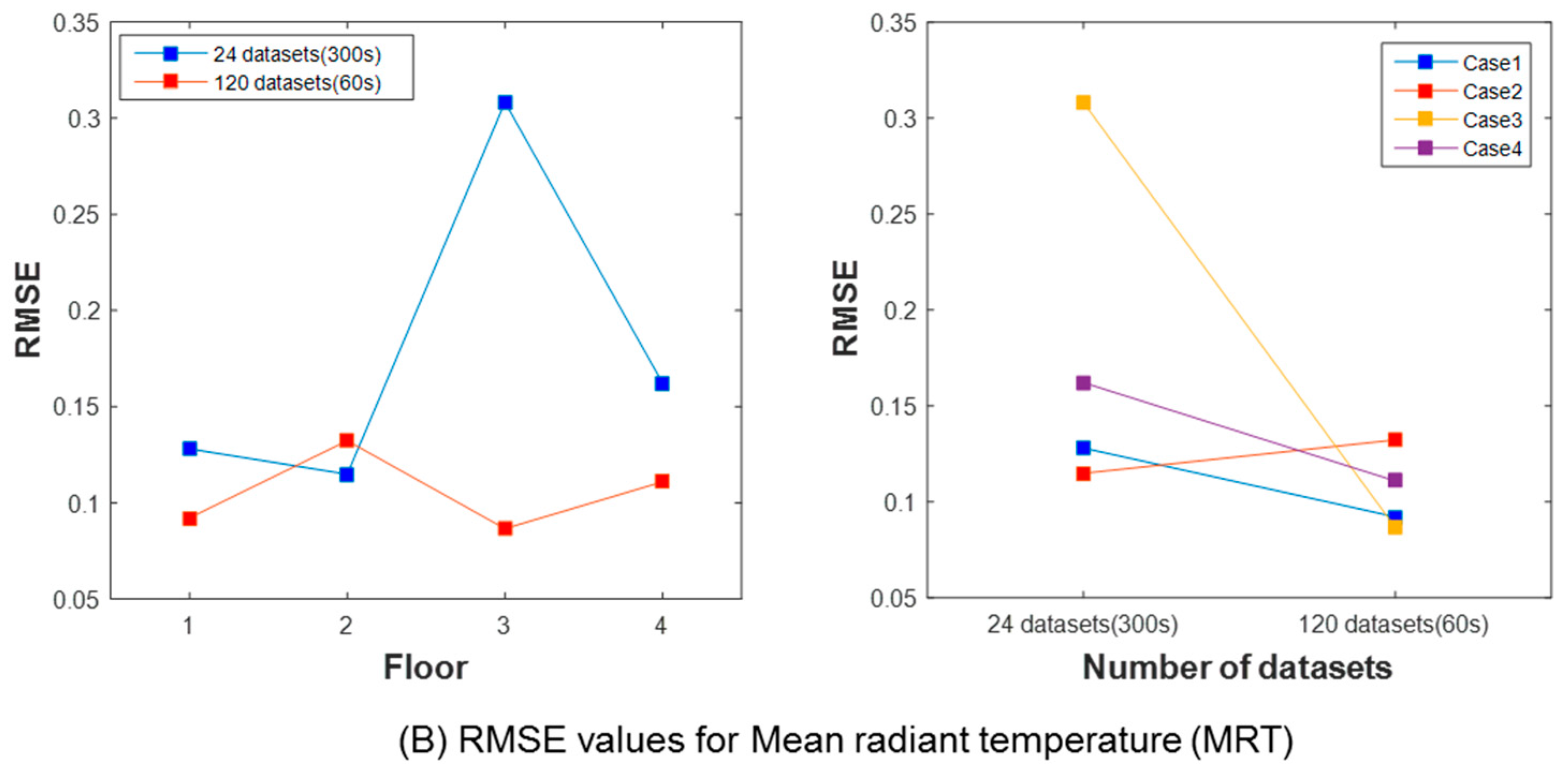
Figure 7A shows the T model’s accuracy on each floor for Cases 1 to 4. R2 was closer to 1 while RMSE and MAE were closer to 0 for Case 2 followed by Cases 1, 4, and 3. Each case’s learning data range (Table 4 and Table 5) demonstrates that accuracy was higher in the floor with smaller data variations (in the order of the second floor, the first floor, the fourth floor, and third floor). We also evaluated the accuracy in Cases 1 to 4 according to the number of data points. For Cases 1 and 2, which had smaller variations in the data, the number of data points did not have a large effect on the model accuracy. By contrast, in Cases 3 and 4, which had large variations, a larger number of data led to higher accuracy. Therefore, the third and fourth floors with larger variations would need more data than the first and second floors.
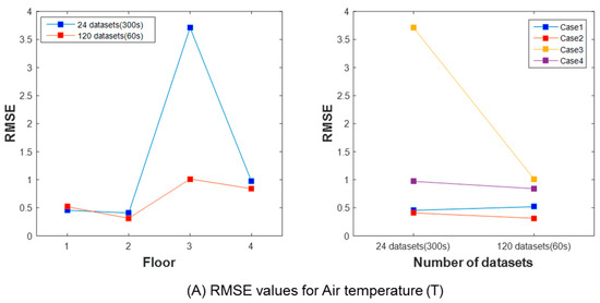
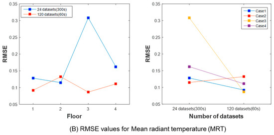
Figure 7.
Results of RMSE for T and MRT prediction models according to the floors and number of datasets.
Figure 7B shows the MRT model’s accuracy for Cases 1 to 4. There was no clear trend in the model accuracy with data variations (smallest in Case 1, followed by Cases 3, 4, and 2), which is attributable to the simulation method. Nonetheless, the error of the model with the same number of data points was lower in the order of Case 3-1 > Case 1-1 > Case 4-1 > Case 2-1 and lower in the order of Case 2-2 > Case 1-2 > Case 4-2 > Case 3-2, confirming that a larger number of data resulted in higher accuracy.
4.2. Evaluation of ANN Model According to the Model Structures
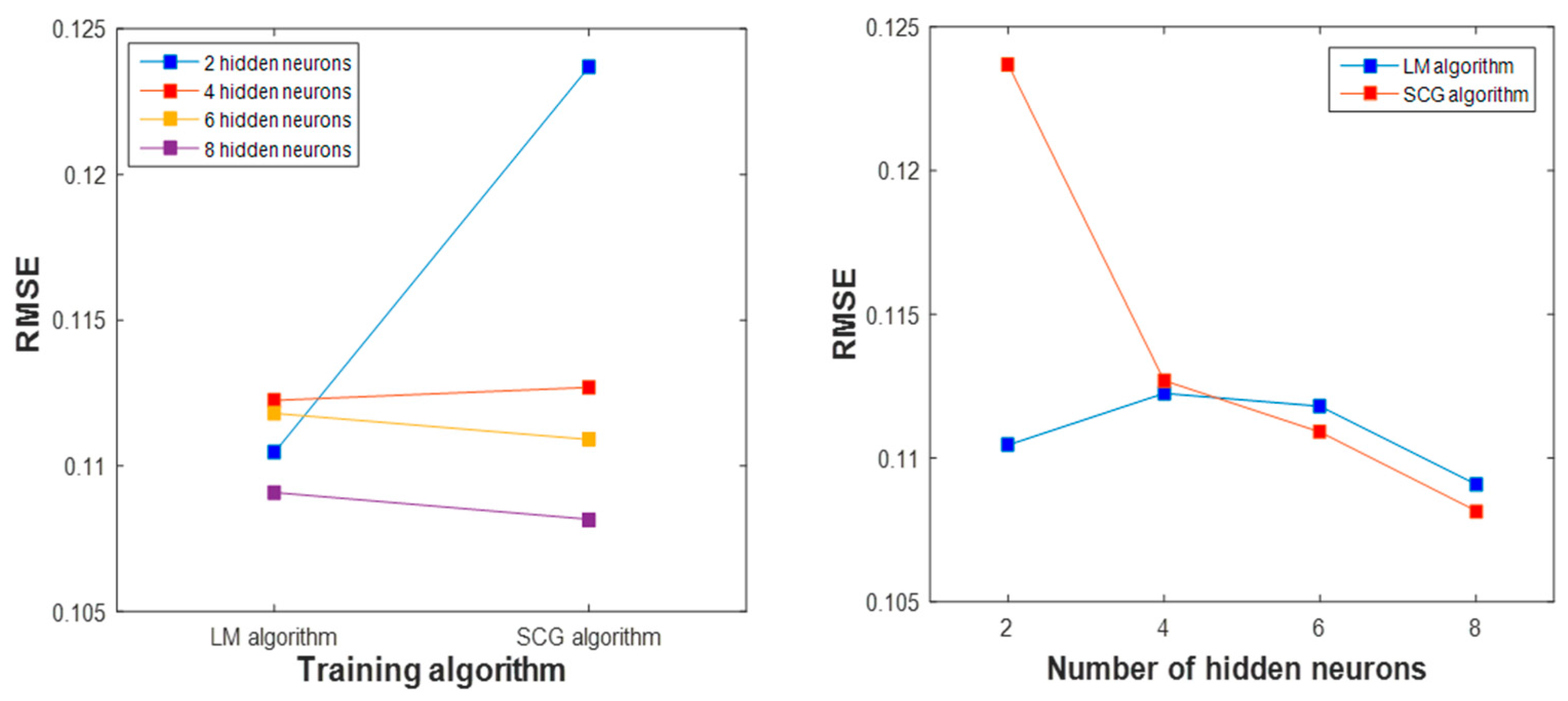
The accuracy of the CLO model was evaluated according to the model structure. For the ANN model cases selected in Section 3.1, the CLO model was developed using the learning dataset of clothing described in Section 3.3 (Table 3, Table 5 and Table 6). This section describes the evaluation of the model accuracy on cases according to the learning algorithm and the number of hidden neurons. Table 7 shows the CLO model accuracy on each case evaluated using the statistical measures of R2, RMSE, and MAE. The clothing learning results showed that the model had the explanatory power of 0.5 and did not vary with the number of hidden neurons. Figure 8 shows that the learning algorithm’s accuracy on Cases 5 and 6, albeit small, was higher in Case 5 than in Case 6 and that the LM algorithm was more accurate. In addition, RMSE value decreased as the number of hidden neurons increased.
Table 7.
Accuracy of CLO prediction models according to the model structures.
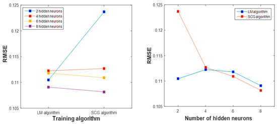
Figure 8.
Results of RMSE for CLO prediction models according to the floors and number of datasets.
An evaluation of the ANN models showed that smaller variations in data and a larger number of learning data points led to a higher level of accuracy. An evaluation of the prediction performance of the three models using the verification data showed that the prediction performance was in the order of CLO model > MRT model > T model. In the MRT and T models, learning data did not fully explain the verification data. The number of hidden neurons did not have a significant effect on the learning accuracy and a structure with one more hidden neuron than the number of input data points would be sufficient as suggested in the literature review.
The result of this study showed the applicability of the ANN model to predict thermal environment in a large space. This method not only enables users to install sensors on easy-to-install locations such as interior wall surface, but also to minimize the number of its installations (See Figure 9). The ANN applied in this study is a highly accurate prediction method and is used in various energy and environmental problems [13,14,26]. However, the prediction performance of the model depends on the learning data in the ANN. In order to increase the prediction accuracy, it is important to obtain learning data that can sufficiently explain the target area’s thermal environment. In practice, the actual building’s thermal environment does not change drastically but tends to show repeated patterns as per the building’s schedule. Therefore, if sufficient data were collected through experiments including testing, adjusting, and balancing (TAB) of a building’s system during commissioning, an ANN model with high prediction performance can be developed.
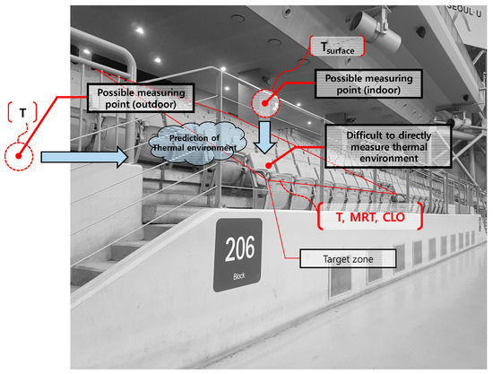
Figure 9.
An example of the method for predicting thermal environment in a large space. In a stadium, it can be difficult to directly install measuring devices on the seats. The ANN based prediction algorithm enables user to install measuring devices on easy-to-install locations.
5. Conclusions
A thermal environment prediction method is proposed using ANN models to evaluate the thermal environment in a large space divided into zones. Three of the six key factors that have a significant effect on the thermal environment felt by the occupants in a large space were the factors to be predicted and the other three were the fixed factors. The three factors to be predicted included indoor temperature, mean radiant temperature, and clothing. To develop ANN models for these three factors, we established learning and verification datasets and built a thermal environment prediction process. We also developed ANN models based on the data characteristics and the model structure and examined their applicability as an effective prediction method.
The prediction method was derived to improve two limitations of the thermal environment evaluation studies of stadiums; it is difficult to install measuring sensors directly on the stands and the stadium stands have different thermal environments depending on the location. Our prediction algorithm used interior wall surface and outdoor air temperature as measurement data; therefore, sensors can be installed in places where it is easy to control them. Furthermore, as the algorithm predicts thermal factors in each zone using ANN models, it can evaluate the thermal environment of the stands depending on the location. The six factors can be used as key input data for thermal environment evaluation indices. The thermal environment evaluation process derived in this study can be used to control HVAC facilities in each zone of a large space building via learning by ANN models.
Acknowledgments
This work was supported by Inha University research grant and this work was supported by a grant (18AUDP-B100345-04) from Architecture & Urban Development Research Program funded by Ministry of Land, Infrastructure and Transport of Korean government.
Author Contributions
Hyun-Jung Yoon and Jae-Hun Jo had the original idea for the study, and all co-authors conceived of and designed the methodology. Hyun-Jung Yoon drafted the manuscript, which was revised by Jae-Hun Jo. All authors read and approved the final manuscript.
Conflicts of Interest
The authors declare no conflict of interest.
References
- Mc Dowall, R. Fundamentals of HVAC Systems; SI Edition; ASHRAE Inc.: Atlanta, GA, USA, 2007. [Google Scholar]
- Jeong, S.J. A Study on the Characteristics and Effective Control of Heat Environment of Large Space; Catholic University of Daegu: Gyeongsan, Korea, 2009. [Google Scholar]
- Kim, D.S.; Cho, Y.J.; Kim, K.H.; Lee, J.H. Case study of thermal environmentin in large space. Mag. SAREK 2001, 30, 25–32. [Google Scholar]
- Fanger, P.O. Thermal Comfort: Analysis and Applications in Environmental Engineering; Danish Technical Press: Copenhagen, Denmark, 1970. [Google Scholar]
- ASHRAE Inc. Standard 55–2010—Thermal Environmental Conditions for Human Occupancy; ASHRAE Inc.: Atlanta, GA, USA, 2010. [Google Scholar]
- ISO. ISO 7730: Ergonomics of the Thermal Environment—Analytical Determination and Interpretation of Thermal Comfort Using Calculation of the PMV and PPD Indices and Local Thermal Comfort Criteria; ISO: Oslo, Norway, 2005. [Google Scholar]
- Kim, S.H.; Yun, S.J.; Chung, K.S. A study on the application of simulation-based simplified pmv regression model for indoor thermal comfort control. J. Energy Eng. 2015, 24, 69–77. [Google Scholar] [CrossRef]
- Tino, P.; Benuskova, L.; Sperduti, A. Artificial neural network models. In Handbook of Computational Intelligence; Springer: Berlin, Germany, 2015. [Google Scholar]
- Karatasou, S.; Santamouris, M.; Geros, V. Modeling and predicting building’s energy use with artificial neural networks: Methods and results. Energy Build. 2006, 38, 949–958. [Google Scholar] [CrossRef]
- Dombaycı, Ö.A.; Gölcü, M. Daily means ambient temperature prediction using artificial neural network method: A case study of Turkey. Renew. Energy 2009, 34, 1158–1161. [Google Scholar] [CrossRef]
- Al Shamisi, M.H.; Assi, A.H.; Hejase, H.A.N. Using MATLAB to develop artificial neural network models for predicting global solar radiation in Al Ain city—UAE. In Engineering Education and Research Using MATLAB; InTech: Rijeka, Croatia, 2011. [Google Scholar] [CrossRef]
- Antoine, G.; Julien, E.; Matthieu, C.; Stéphane, G. HVAC control and comfort management in non-residential buildings. In Proceedings of the 13th Conference of International Building Performance Simulation Association, Chambéry, France, 26–28 August 2013. [Google Scholar]
- Ferreira, P.M.; Ruano, A.E.; Silva, S.; Conceicao, E.Z.E. Neural networks based predictive control for thermal comfort and energy savings in public buildings. Energy Build. 2012, 55, 238–251. [Google Scholar] [CrossRef]
- Castilla, M.; Álvarez, J.D.; Ortega, M.G.; Arahal, M.R. Neural network and polynomial approximated thermal comfort models for HVAC systems. Build. Environ. 2013, 59, 107–115. [Google Scholar] [CrossRef]
- ASHRAE. Handbook of Fundamentals; American Society of Heating Refrigerating and Air Conditioning Engineers: Atlanta, GA, USA, 2005. [Google Scholar]
- Seok, H.T.; Kim, H.J.; Choi, D.H.; Chae, M.B.; Yang, J.H. A study on the comparison analysis of the field measurement and CFD simulation in dome stadium. J. Arch. Inst. Korea Plan. Des. 2009, 25, 357–364. [Google Scholar]
- Kim, D.S. Nueral Networks Theory and Applications 1; Dongnimmun-ro 14-gil: Seoul, Korea, 2006. [Google Scholar]
- Yoon, H.J.; Kim, E.J.; Jo, J.H. Development of smart sensors with implemented objective function to the indoor and outdoor environmental data. In Proceedings of the 9th International Conference on Indoor Air Quality Ventilation & Energy Conservation in Buildings, Seoul, Korea, 23–26 October 2016. [Google Scholar]
- Mark, H.B.; Martin, T.H.; Howard, B.D. R2016b NN User’s Guide; MathWorks: Natick, MA, USA, 2016. [Google Scholar]
- Carpenter, W.C.; Barthelemy, J.F. Common misconceptions about neural networks as approximators. J. Comput. Civ. Eng. 1994, 8, 345–358. [Google Scholar] [CrossRef]
- Seok, H.T.; Chae, M.B.; Choi, D.H. Measurement examination of indoor thermal environment characteristic in accordance with heat loads from occupant for large enclosure in winter. J. Korean Assoc. Spat. Struct. 2007, 7, 97–107. [Google Scholar]
- CATIA. Dassault Systems. Available online: http://www.3ds.com (accessed on 3 August 2016).
- STAR-CCM+. Siemens. Available online: http://mdx.plm.automation.siemens.com (accessed on 5 November 2016).
- Kim, S.S. Evaluation of the thermal environment in a theater using CFD. In Daewoo Construction Technology Report; Daewoo construction: Suwon-si, Gyeonggi-do, Korea, 2005. [Google Scholar]
- Chen, Y.Y. Energy Metabolism & Body Temperature; Zhengzhou University: Zhengzhou, China, 2005; Chapter 16. [Google Scholar]
- Atthajariyakul, S.; Leephakpreeda, T. Neural computing thermal comfort index for HVAC systems. Energy Convers. Manag. 2005, 46, 2553–2565. [Google Scholar] [CrossRef]
- ASHRAE RP884. The University of Sydney Database Downloader. Available online: http://sydney.edu.au (accessed on 5 June 2016).

© 2018 by the authors. Licensee MDPI, Basel, Switzerland. This article is an open access article distributed under the terms and conditions of the Creative Commons Attribution (CC BY) license (http://creativecommons.org/licenses/by/4.0/).