Harmonic Spectrum of Output Voltage for Space Vector Pulse Width Modulated Ultra Sparse Matrix Converter

Abstract

In a matrix converter, the frequencies of output voltage harmonics are related to the frequencies of input, output, and carrier signals, which are independent of each other. This nature may cause an inaccurate harmonic spectrum when using conventional analytical methods, such as fast Fourier transform (FFT) and the double Fourier analysis. Based on triple Fourier series, this paper proposes a method to pinpoint harmonic components of output voltages of an ultra sparse matrix converter (USMC) under space vector pulse width modulation (SVPWM) strategy. Amplitudes and frequencies of harmonic components are determined precisely for the first time, and the distribution pattern of harmonics can be observed directly from the analytical results. The conclusions drawn in this paper may contribute to the analysis of harmonic characteristics and serve as a reference for the harmonic suppression of USMC. Besides, the proposed method is also applicable to other types of matrix converters.

1. Introduction

The ultra-sparse matrix converter (USMC) evolved from the conventional matrix converter (CMC) and inherited many merits from CMC including compact structure without intermediate storage, sinusoidal input and output current, adjustable input power factor, etc. Meanwhile, USMC possesses superiorities over CMC, such as simpler commutation technology, a decrease in number of switches, etc. Currently, USMC is considered as a promising type of matrix converter [1,2,3,4].

As an AC–AC power converter, the primary task of USMC is to obtain a sinusoidal output waveform with high quality. However, due to the characteristics of the power device and the modulation methods, the output voltages of USMC inevitably contain harmonic components, thus negatively impacting the practical application. Therefore, it is very important to analyze the harmonic components in the output waveform of USMC, which not only lays the foundation for the suppression of the harmonics but also improves the theory concerning matrix converter harmonic analysis.

Up to now, there are some studies on the harmonic analysis of power electronics converters. Among them, fast Fourier transform (FFT) analysis is the most commonly used one [5,6,7,8]. It is simple and easy to implement. However, FFT involves sampling and window etc. in the processing, which will incur spectrum leakage, aliasing, and other issues. Therefore, when the frequencies of input, output and carrier signals are special, the results of FFT analysis are not accurate. Another commonly used method is calculating the analytical formula with Fourier series. In 1975, S. Bayes and B.M. Bird first applied the double Fourier analysis method to power electronic converters which were originally used in the communication system [9]. Since then, the studies on harmonic analytic solution have mostly concentrated on the double Fourier analysis. For example, the harmonic analytical formulas of output voltage of two-level inverter are derived in [10] by using double Fourier analysis and then a comparison about the high-frequency harmonics is carried out when using saw-tooth carrier and triangular carrier in modulation process. In [11], Jacobi matrix is used to find the closed solution of the double Fourier series; and the characteristics of output voltage of the inverter under different space vector pulse width modulation (SVPWM) are compared. In [12] the output voltage harmonics of inverters with different topologies under various modulation methods are analyzed in detail by double Fourier analysis.

Like CMC, the output voltage of USMC is related to the frequencies of input, output and carrier signals, which are independent of each other. If using double Fourier series analysis, only two of these frequencies are considered at most, resulting in inaccurate spectral analytic results. In view of this problem, some scholars have tried to use triple Fourier series to analyze the harmonic of output waveform for CMC under “AV method” [13,14]. However, due to some differences in the topology and control performance between USMC and CMC, a mature harmonic analysis theory for USMC has yet to emerge. Compared with “AV method”, SVPWM not only increases the maximum voltage transmission ratio from 0.5 to 0.866, but also achieves digitization easily. As a result, SVPWM is currently widely applied [15,16,17]. Therefore, for USMC, the harmonic analysis of output voltage under SVPWM is of important significance.

In this paper, based on the characteristics of SVPWM and triple Fourier series, an output voltage harmonic calculation method for USMC is proposed, which can obtain an accurate harmonic spectrum and identify the relations between the frequencies of harmonic components and the frequencies of input, output and carrier signals. In addition, the harmonic distribution pattern and the main harmonic components of output voltage of USMC are analyzed and summarized according to the analytical results.

2. Triple Fourier Series

It is assumed that the three-variable function g(x, y, z) is periodic in x, y, and z directions with the period of 2π, x, y and z being independent of each other. The triple Fourier series expression of g(x, y, z) can be defined by the following:

$$g(x,y,z)={\displaystyle \sum _{k=-\infty }^{+\infty }{\displaystyle \sum _{p=-\infty }^{+\infty }{\displaystyle \sum _{q=-\infty }^{+\infty }{\mathit{F}}_{kpq}}}}{\mathrm{e}}^{\mathrm{j}\left(kx+py+qz\right)}$$

(1)

where k, p, q are indices on the carrier frequency, output frequency and input frequency respectively; F_kpq is the triple Fourier coefficient and its expression is

$${\mathit{F}}_{kpq}=\frac{1}{8{\mathsf{\pi }}^3}{\displaystyle \int {\displaystyle \int {\displaystyle {\int }_0^{2\mathsf{\pi }}g(x,y,z){\mathrm{e}}^{-\mathrm{j}\left(kx+py+qz\right)}\mathrm{d}x\mathrm{d}y\mathrm{d}z}}}$$

(2)

Let x = 2πf_ct, y = 2πf_outt + φ₀, z = 2πf_int + φ_i then Equation (1) can be regarded as the output voltage expression of any phase of USMC.; f_c, f_out and f_in are respectively carrier frequency, output voltage frequency and input voltage frequency of USMC; φ_i is the input power factor angle; φ₀ is the output voltage initial phase. In most applications, USMC is required to operate with unit power factor, so φ_i = 0. When φ_o is not zero, the integration limits of Equation (2) should be adjusted. Since the integrand g(x, y, z) is periodic in x, y, and z directions with the period of 2π, the integration results would not be affected by the specific values of the integral limits as long as the periodic variation of x, y and z over 2π intervals. Therefore, whether φ₀ is zero does not have any effects on the calculation results. To simplify calculation, it is assumed that φ₀ = 0.

Expending Equation (1) and it can be expressed in the following form:

$$\begin{array}{ll}g(x,y,z)& =\frac{A_{000}}{2}+\left[\begin{array}{l}{\displaystyle \sum _{k=1}^{+\infty }\left[A_{k00}\cos \right(kx)+B_{k00}\cos (kx\left)\right]}+\hfill \\ {\displaystyle \sum _{p=1}^{+\infty }\left[A_{0p0}\cos \right(py)+B_{0p0}\cos (py\left)\right]}+\hfill \\ {\displaystyle \sum _{q=1}^{+\infty }\left[A_{00q}\cos \right(q\mathrm{z})+B_{00q}\cos (q\mathrm{z}\left)\right]}\hfill \end{array}\right]\\ & +\left[\begin{array}{l}{\displaystyle \sum _{k=1}^{+\infty }{\displaystyle \sum _{\begin{array}{l}p=-\infty \\ p\ne 0\end{array}}^{+\infty }\left[A_{kp0}\cos \right(kx+py)+B_{kp0}\sin (kx+py\left)\right]+}}\hfill \\ {\displaystyle \sum _{p=1}^{+\infty }{\displaystyle \sum _{\begin{array}{l}q=-\infty \\ q\ne 0\end{array}}^{+\infty }\left[A_{0pq}\cos \right(py+qz)+B_{0pq}\sin (py+qz\left)\right]+}}\hfill \\ {\displaystyle \sum _{k=1}^{+\infty }{\displaystyle \sum _{\begin{array}{l}q=-\infty \\ q\ne 0\end{array}}^{+\infty }\left[A_{k0q}\cos \right(kx+qz)+B_{k0q}\sin (kx+qz\left)\right]}}\hfill \end{array}\right]\\ & +{\displaystyle \sum _{k=1}^{+\infty }{\displaystyle \sum _{\begin{array}{l}p=-\infty \\ p\ne 0\end{array}}^{+\infty }{\displaystyle \sum _{\begin{array}{l}q=-\infty \\ q\ne 0\end{array}}^{+\infty }\left[\begin{array}{l}{A}_{kpq}\cos \left(kx+py+qz\right)+\\ B_{kpq}\sin \left(kx+py+qz\right)\end{array}\right]}}}\end{array}$$

(3)

In Equation (3) harmonic components are divided into four parts: the first part is the DC component (k = 0, p = 0, q = 0); the second part is the fundamental voltage (k = 0, p = 1, q = 0) and harmonic components only associated with the carrier frequency (when k = 1, 2, 3, …, p = 0, q = 0), the input frequency (when k = 0, p = 0, q = 1, 2, 3, …) or the output frequency (k = 0, p = 2, 3 …, q = 0) respectively; the third part is the harmonic components related to any two of the three frequencies(input, output, and carrier frequencies), and their frequencies are the sum of the integral multiple of the two frequencies; the fourth part is the harmonic components relevant to the three frequencies, and their frequencies are sums of the integral multiples of the three frequencies.

According to the Fourier analysis theory, the frequency of any harmonic is kf_c ± pf_out ± qf_in and the harmonic amplitude U_kpq satisfies the following relationship with F_kpq:

$$U_{kpq}=2\left|{\mathit{F}}_{kpq}\right|$$

(4)

3. Harmonic Calculation of Output Voltage of USMC Under SVPWM Strategy

3.1. SVPWM

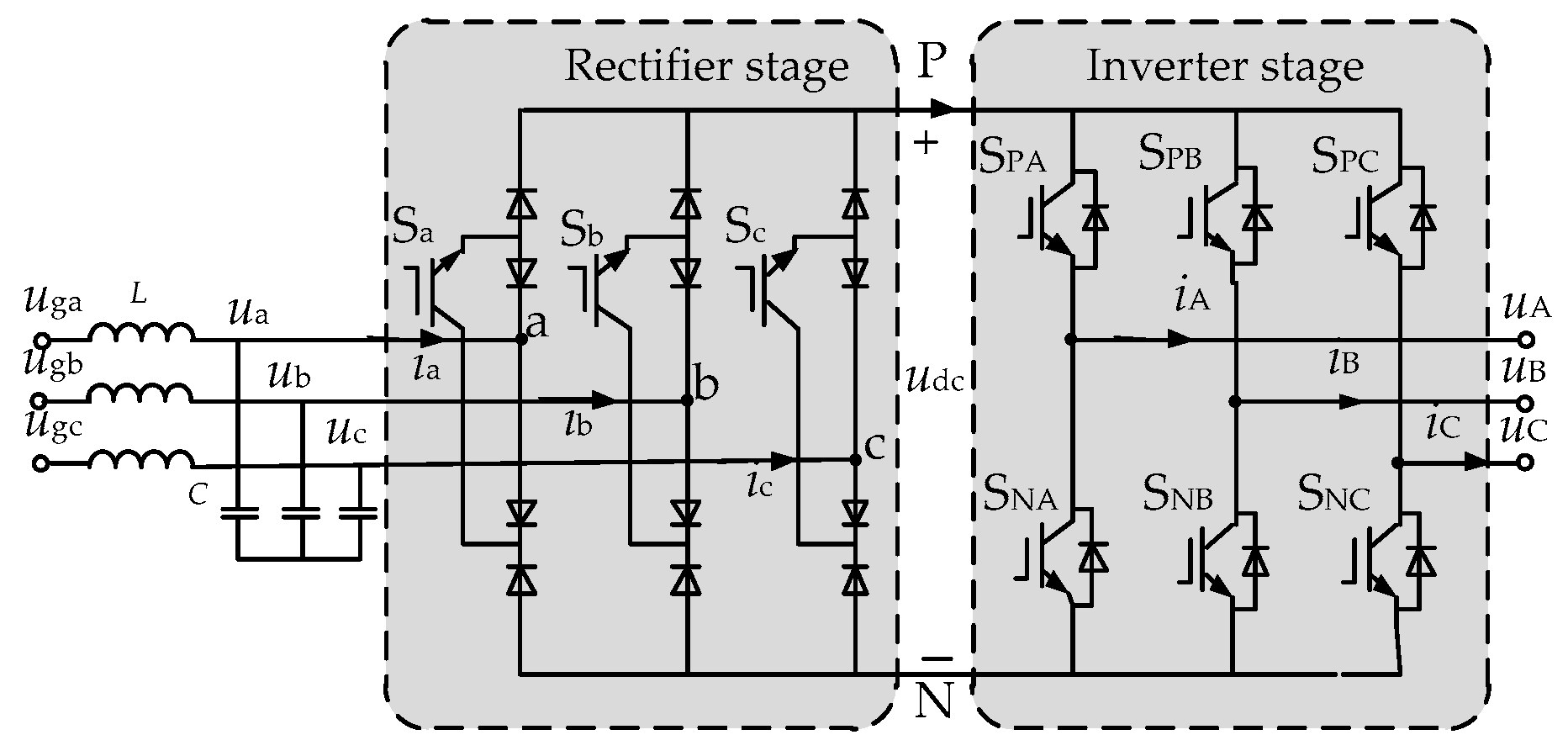
The topology of USMC is shown in Figure 1, which is divided into two stages, the rectifier stage and the inverter stage. There are three phases in rectifier stage, each of which consists of one unidirectional IGBT and four diodes. The inverter stage has the same structure as the traditional two-level voltage source inverter.

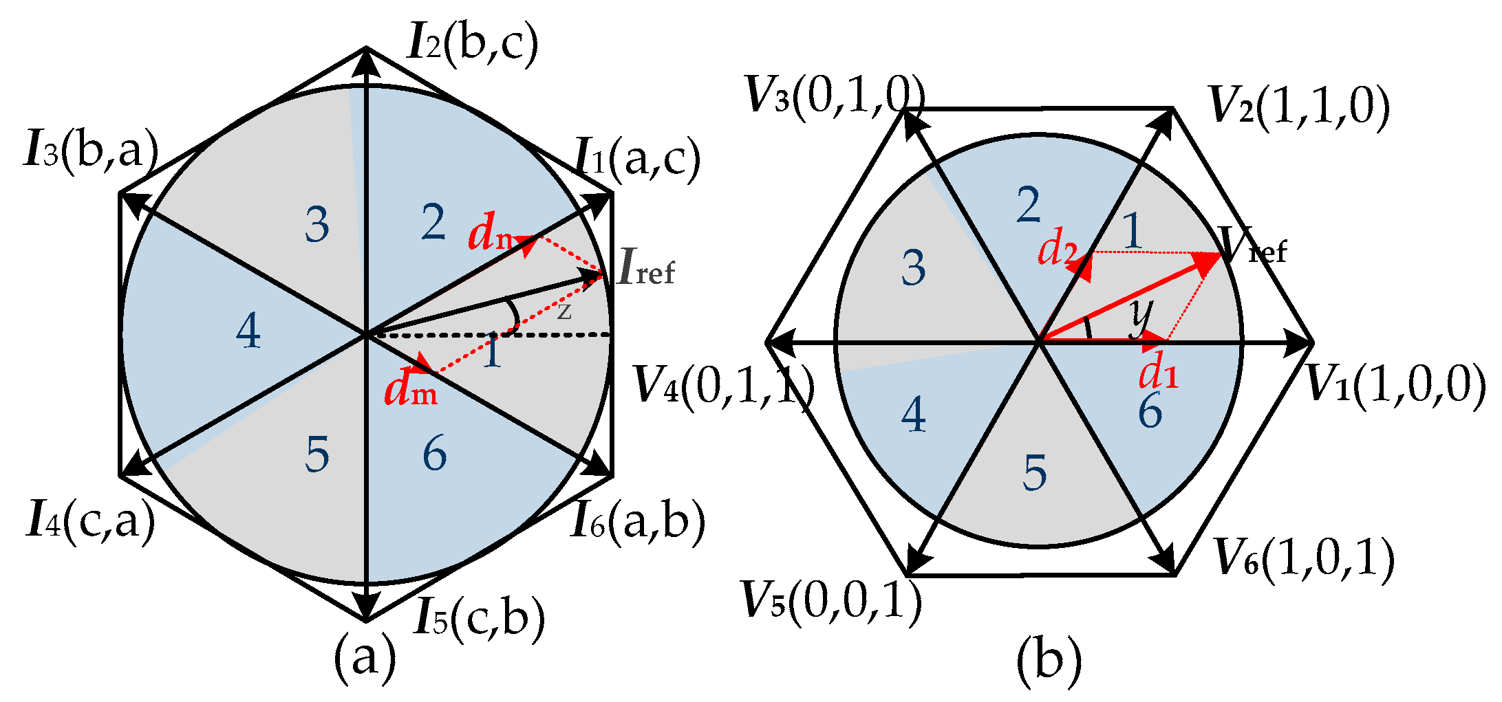
The SVPWM strategy of rectifier stage is shown in Figure 2a, in which the six effective vectors I₁–I₆ divide the space into six sectors. Taking I₁(a, c) as an example, “a” represents that S_a and S_c are on-state, while S_b is off-state. In each sector, there is always one phase remaining the maximum current amplitude in the rectifier stage. In order to obtain the maximum voltage utilization, the switching device corresponding to maximum current amplitude is kept open, and the other two switches are switched on alternately. The duty cycles of the two adjacent effective vectors required to synthesize the reference input current vector I_ref can be obtained by the following equation:

$$\{\begin{array}{l}{d}_{\mathrm{m}}=\frac{\sin \left[\frac{\mathsf{\pi }}{3}-z-\frac{\mathsf{\pi }}{6}+\frac{\mathsf{\pi }}{3}\left(k_{\mathrm{in}}-1\right)\right]}{\cos \left[z-\frac{\mathsf{\pi }}{3}(k_{\mathrm{in}}-1)\right]}\\ d_{\mathrm{n}}=\frac{\sin \left[z+\frac{\mathsf{\pi }}{6}-\frac{\mathsf{\pi }}{3}\left(k_{\mathrm{in}}-1\right)\right]}{\cos \left[z-\frac{\mathsf{\pi }}{3}(k_{\mathrm{in}}-1)\right]}\end{array}$$

(5)

where k_in is the sector number of the reference input current vector.

When I_ref is in the first sector, the expression of average DC voltage u_dc in a carrier cycle is as follows:

$$u_{\mathrm{dc}}=d_{\mathrm{m}}{u}_{\mathrm{ab}}+d_{\mathrm{n}}{u}_{\mathrm{ac}}=\frac{3U_{\mathrm{im}}}{2\cos z}$$

(6)

where u_ab and u_ac are input line voltage, u_ab = $\sqrt{3}$U_imcos(z + π/6), u_ac = $\sqrt{3}$U_imcos(z − π/6); U_im is the amplitude of input phase voltage.

Similarly, when I_ref is in other sectors, the values of u_dc and the duty cycles d_a, d_b and d_c of the switches S_a, S_b and S_c can be obtained as shown in

Table 1. The expression of d_a, d_b, and d_c when I_ref in diffirent vectors.

z	kin	da	db	dc	udc
[−π/6,π/6)	1	1	dm	dn	3Uim/2cosz
[π/6,π/2)	2	dm	dn	1	−3Uim/2cos(z + 2π/3)
[π/2,5π/6)	3	dn	1	dm	3Uim/2cos(z − 2π/3)
[5π/6,7π/6)	4	1	dm	dn	−3Uim/2cosz
[7π/6,3π/2)	5	dm	dn	1	3Uim/2cos(z + 2π/3)
[3π/2,11π/6)	6	dn	1	dm	−3Uim/2cos(z − 2π/3)

.

Figure 2b shows the SVPWM strategy of inverter stage, in which the six effective vectors V₁–V₆ divide the space vector into six sectors. Taking V₁(1, 0, 0) as an example, “1” means that S_pA is on-state in the upper bridge arm of phase A; and the second and third bits “0” represent that S_NB and S_NC are turned on in the lower bridge arm of phase B and phase C respectively. The duty cycles of the two adjacent effective vectors and zero vectors required to synthesize the reference output voltage vector V_ref can be obtained by the following equation:

$$\{\begin{array}{l}{d}_1=\frac{\sqrt{3}{U}_{\mathrm{ref}}}{u_{\mathrm{dc}}}\sin \left[\frac{\mathsf{\pi }}{3}-y+\frac{\mathsf{\pi }}{3}(k_{\mathrm{out}}-1)\right]\\ d_2=\frac{\sqrt{3}{U}_{\mathrm{ref}}}{u_{\mathrm{dc}}}\sin \left[y-\frac{\mathsf{\pi }}{3}(k_{\mathrm{out}}-1)\right]\\ d_0=1-d_1-d_2\end{array}$$

(7)

where k_out is the sector number of the reference output voltage vector, U_ref is the amplitude of output phase voltage.

The duty cycles of S_Pμ (μ = A, B, C) are defined as d_Pμ. When V_ref is located in different sectors, the values of d_Pμ are shown in

Table 2. The expression of d_Pμ when V_ref is in different vectors.

y	kout	dPA	dPB	dPC
[0,π/3)	1	(1 + d1 + d2)/2	(1 − d1 + d2)/2	(1 − d1 − d2)/2
[π/3,2π/3)	2	(1 + d1 − d2)/2	(1 + d1 + d2)/2	(1 − d1 − d2)/2
[2π/3,π)	3	(1 − d1 − d2)/2	(1 + d1 + d2)/2	(1 − d1 + d2)/2
[π,4π/3)	4	(1 − d1 − d2)/2	(1 + d1 − d2)/2	(1 + d1 + d2)/2
[4π/3,5π/3)	5	(1 − d1 + d2)/2	(1 − d1 − d2)/2	(1 + d1 + d2)/2
[5π/3,2π)	6	(1 + d1 + d2)/2	(1 − d1 − d2)/2	(1 + d1 − d2)/2

. Since the conducting state of upper and lower bridge arm switches in the same phase of A, B and C are complementary, the duty cycles of S_Pμ and S_Nμ satisfy the following relationship: d_Nμ = 1 − d_Pμ.

3.2. Harmonic Calculation of Output Voltage

Since the three-phase output voltages of USMC are symmetrical, the following calculation and analysis take Phase A as an example. It can be seen from Equation (4) that the amplitude corresponding to each harmonic can be determined by the value of Fourier coefficients. Considering the SVPWM process, the integration limit can be redefined without altering the analytical solution, requiring only cyclic variation of x, y and z over 2π intervals. So the expression of F_{A_kpq} in Equation (2) can be defined as follows:

$${\mathit{F}}_{\mathrm{A}\_}{}_{kpq}=\frac{1}{8{\mathsf{\pi }}^3}{\displaystyle {\int }_{\frac{-\mathsf{\pi }}{6}}^{\frac{11\mathsf{\pi }}{6}}{\displaystyle {\int }_0^{2\mathsf{\pi }}{\displaystyle {\int }_{-\mathsf{\pi }}^{\mathsf{\pi }}{u}_{\mathrm{A}}{\mathrm{e}}^{-\mathrm{j}\left(kx+py+qz\right)}\mathrm{d}x\mathrm{d}y\mathrm{d}z}}}$$

(8)

In the operation process of USMC, u_A is actually a pulse wave. Therefore, to solve Equation (8), it is necessary to determine the trip point of the output voltage pulse and the value of u_A. The following is the process to solve various trip points of output voltage pulse based on the analysis of SVPWM of USMC.

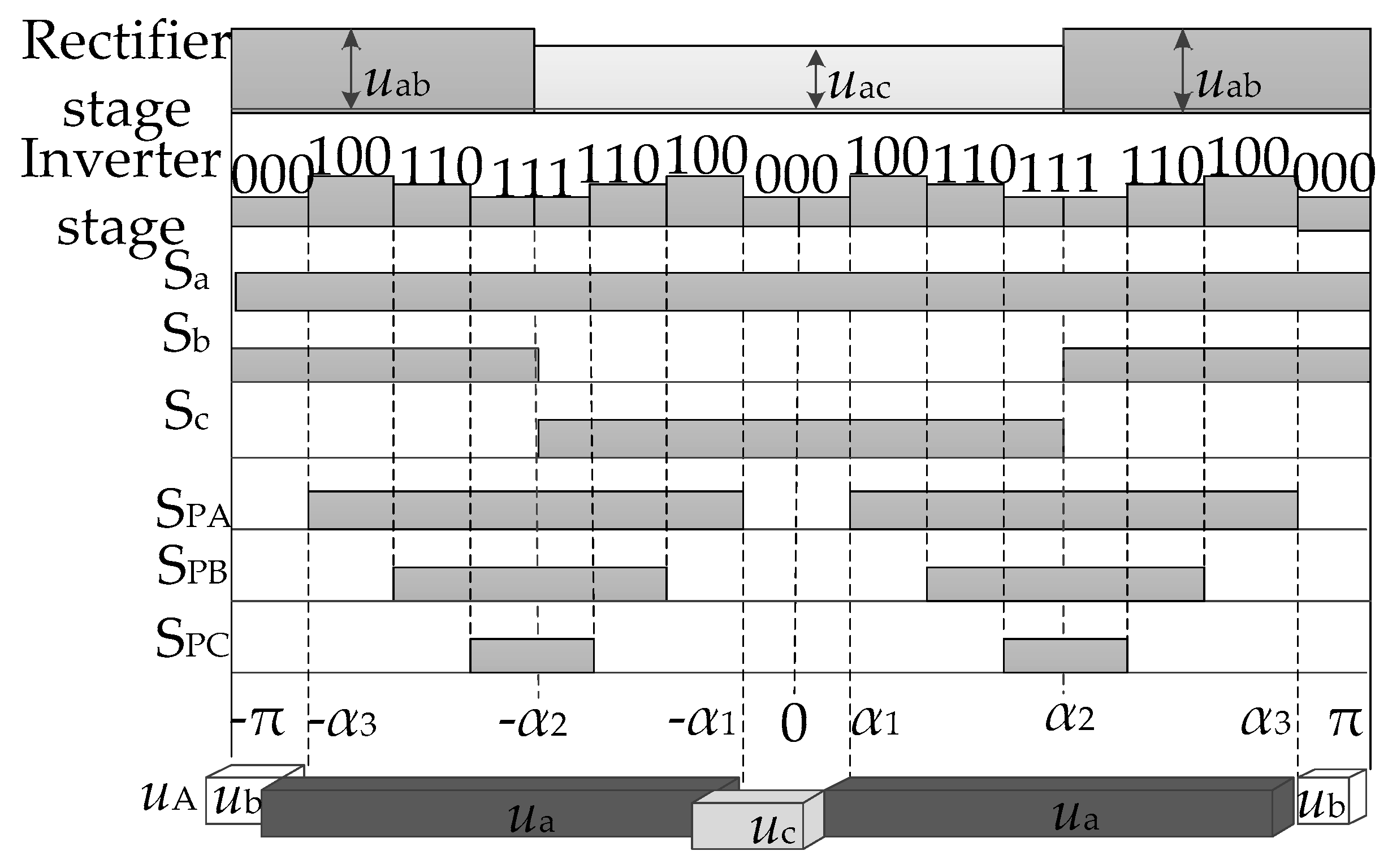
When both the reference input current vector I_ref and output voltage vector V_ref are in the first sector, the conduction state of each switch in one carrier period and instantaneous value of A-phase output voltage can be determined based on the switching sequence of the rectification stage and the inverter stage, as shown in Figure 3.

It should be noted that this paper is aimed at symmetrical regularly sampled SVPWM. The carrier function c(x) used in this paper can be expressed as:

$$c(x)=\frac{1}{\mathsf{\pi }}\cdot \arccos (\cos x),x\in \left[-\mathsf{\pi },\mathsf{\pi }\right]$$

(9)

Combine the duty cycle of each switch with Equation (9), and α₁, α₂ and α₃ in Figure 3 can be determined as follows:

$$\{\begin{array}{l}{\alpha }_1=d_{\mathrm{NA}}{d}_{\mathrm{n}}=(1-d_{\mathrm{PA}})d_{\mathrm{n}}\mathsf{\pi }\\ {\alpha }_2=d_{\mathrm{n}}\mathsf{\pi }\\ {\alpha }_3=\left(d_{\mathrm{n}}+d_{\mathrm{PA}}{d}_{\mathrm{m}}\right)\mathsf{\pi }\end{array}$$

(10)

When the reference vectors of input current and output voltage are located in other sectors, the values of α₁, α₂ and α₃ can be analyzed in a similar way. It is found that the expressions of α₁, α₂ and α₃ are the same when I_ref and V_ref are in different sectors, except that the specific values of d_PA, d_m and d_n are changed with k_in or k_out.

Based on the above analysis, Equation (8) can be further simplified as follows:

$${\mathit{F}}_{\mathrm{A}\text{\_}kpq}={\mathit{F}}_{\mathrm{A}1}+{\mathit{F}}_{\mathrm{A}2}$$

(11)

where

$${\mathit{F}}_{\mathrm{A}1}=\frac{1}{8{\mathsf{\pi }}^3}{\displaystyle \sum _{k_{\mathrm{in}}=1,3,5}{\displaystyle \sum _{k_{\mathrm{out}}=1}^6{\displaystyle {\int }_{z_{\mathrm{r}}}^{z_{\mathrm{f}}}{\displaystyle {\int }_{y_{\mathrm{r}}}^{y_{\mathrm{f}}}{D}_1\cdot {\mathrm{e}}^{-\mathrm{j}\left(py+qz\right)}\mathrm{d}y}}\mathrm{d}z}}$$

(12)

$${\mathit{F}}_{\mathrm{A}2}=\frac{1}{8{\mathsf{\pi }}^3}{\displaystyle \sum _{k_{\mathrm{in}}=2,4,6}{\displaystyle \sum _{k_{\mathrm{out}}=1}^6{\displaystyle {\int }_{z_{\mathrm{r}}}^{z_{\mathrm{f}}}{\displaystyle {\int }_{y_{\mathrm{r}}}^{y_{\mathrm{f}}}{D}_2\cdot {\mathrm{e}}^{-\mathrm{j}\left(py+qz\right)}\mathrm{d}y}}\mathrm{d}z}}$$

(13)

where

$$\begin{array}{ll}{D}_1& ={\displaystyle {\int }_{-\mathsf{\pi }}^{-{\alpha }_3}{u}_{\mathrm{A}1}{\mathrm{e}}^{-\mathrm{j}kx}\mathrm{d}x}+{\displaystyle {\int }_{-{\alpha }_3}^{-{\alpha }_1}{u}_{\mathrm{A}2}{\mathrm{e}}^{-\mathrm{j}kx}\mathrm{d}x}+{\displaystyle {\int }_{-{\alpha }_1}^{{\alpha }_1}{u}_{\mathrm{A}3}{\mathrm{e}}^{-\mathrm{j}kx}\mathrm{d}x}\\ & +{\displaystyle {\int }_{{\alpha }_1}^{{\alpha }_3}{u}_{\mathrm{A}4}{\mathrm{e}}^{-\mathrm{j}kx}\mathrm{d}x}+{\displaystyle {\int }_{{\alpha }_3}^{\mathsf{\pi }}{u}_{\mathrm{A}5}{\mathrm{e}}^{-\mathrm{j}kx}\mathrm{d}x}\end{array}$$

(14)

$$\begin{array}{ll}{D}_2& ={\displaystyle {\int }_{-\mathsf{\pi }}^{-{\alpha }_3}{u}_{\mathrm{A}1}{\mathrm{e}}^{-\mathrm{j}kx}\mathrm{d}x}+{\displaystyle {\int }_{-{\alpha }_3}^{-{\alpha }_2}{u}_{\mathrm{A}2}{\mathrm{e}}^{-\mathrm{j}kx}\mathrm{d}x}+{\displaystyle {\int }_{-{\alpha }_2}^{-{\alpha }_1}{u}_{\mathrm{A}3}{\mathrm{e}}^{-\mathrm{j}kx}\mathrm{d}x}\\ & +{\displaystyle {\int }_{-{\alpha }_1}^{{\alpha }_1}{u}_{\mathrm{A}4}{\mathrm{e}}^{-\mathrm{j}kx}\mathrm{d}x}+{\displaystyle {\int }_{{\alpha }_1}^{{\alpha }_2}{u}_{\mathrm{A}5}{\mathrm{e}}^{-\mathrm{j}kx}\mathrm{d}x}+{\displaystyle {\int }_{{\alpha }_2}^{{\alpha }_3}{u}_{\mathrm{A}6}{\mathrm{e}}^{-\mathrm{j}kx}\mathrm{d}x}\\ & +{\displaystyle {\int }_{{\alpha }_3}^{\mathsf{\pi }}{u}_{\mathrm{A}7}{\mathrm{e}}^{-\mathrm{j}kx}\mathrm{d}x}\end{array}$$

(15)

The integration limits z_r and z_f in Equations (12) and (13), and the values of u_Aλ (λ = 1–7) in Equations (14) and (15) are related to the sector number of reference input current as shown in

Table 3. Value of u_Aλ, z_r and z_f when k_in changes from 1 to 6.

kin	zr	zf	uA1	uA2	uA3	uA4	uA5	uA6	uA7
1	−π/6	π/6	ub	ua	uc	ua	ub	-	-
2	π/6	π/2	uc	ua	ub	uc	ub	ua	uc
3	π/2	5π/6	uc	ub	ua	ub	uc	-	-
4	5π/6	7π/6	ua	ub	uc	ua	uc	ub	ua
5	7π/6	3π/2	ua	uc	ub	uc	ua	-	-
6	3π/2	11π/6	ub	uc	ua	ub	ua	uc	ub

.; y_r and y_f in Equations (12) and (13) are related to the sector number of reference output voltage, as shown in

Table 4. Value of y_r and y_f when k_out change from 1 to 6.

kout	1	2	3	4	5	6
yr	0	π/3	2π/3	π	4π/3	5π/3
yf	π/3	2π/3	π	4π/3	5π/3	2π

.

Based on Equations (11) and (15), the analytical solution of F_{A_kpq} can be obtained by further calculation in MATLAB; then the amplitude of each harmonic can be got.

4. Spectrum Analysis of Harmonic Characteristics of Output Voltage of USMC

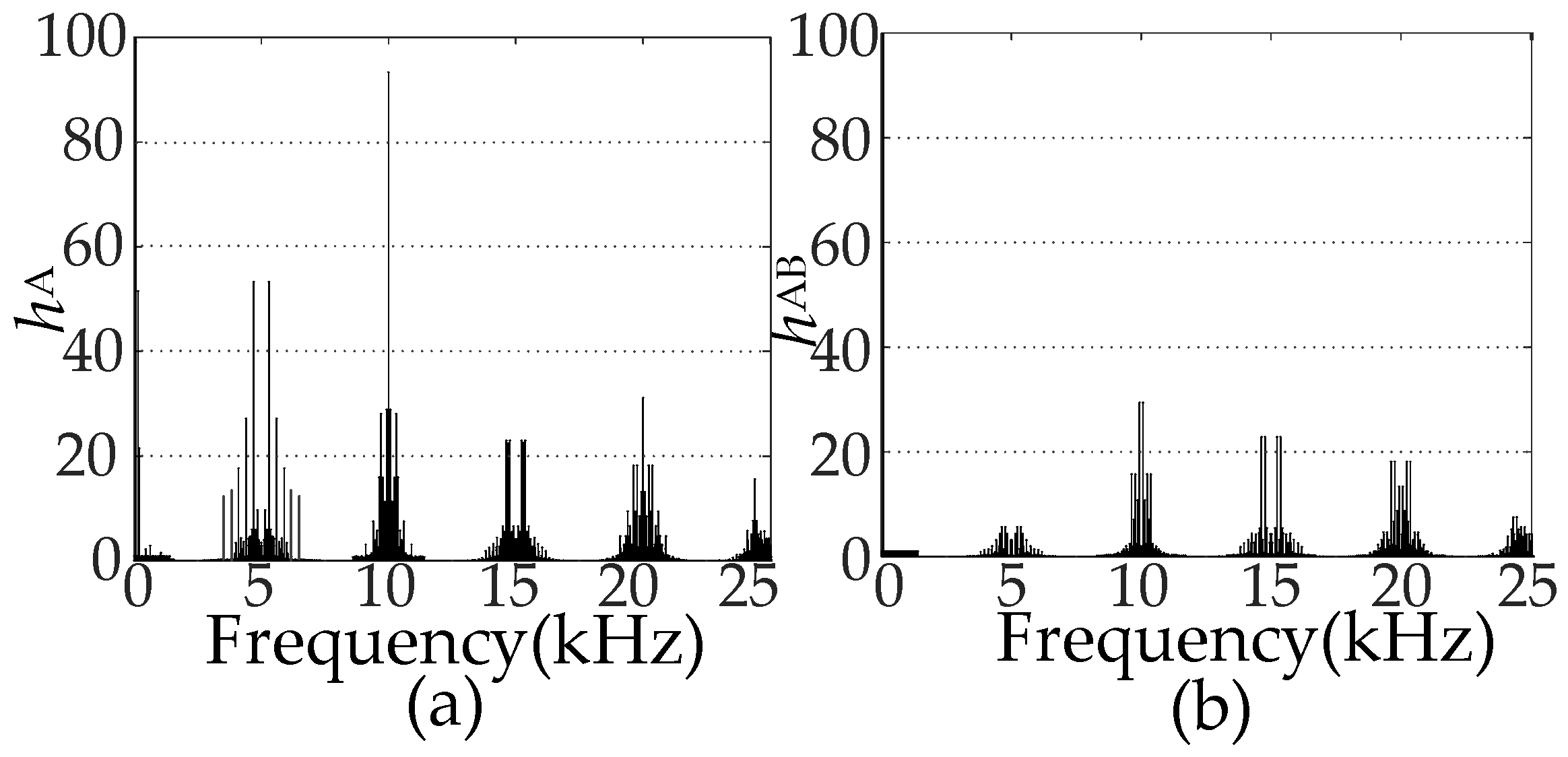
When the voltage transmission ratio m is 0.5 (m is the ratio of U_ref/U_im), the input frequency f_in is 50 Hz, the output frequency f_out is 70 Hz and the carrier frequency f_c is 5 kHz, the analytical spectrums of output phase voltage u_A and line voltage u_AB can be obtained by the calculation formula in Section 3. The spectrums are shown in Figure 4, where h_A and h_AB are normalized values based on the fundamental amplitude of phase voltage and line voltage respectively. 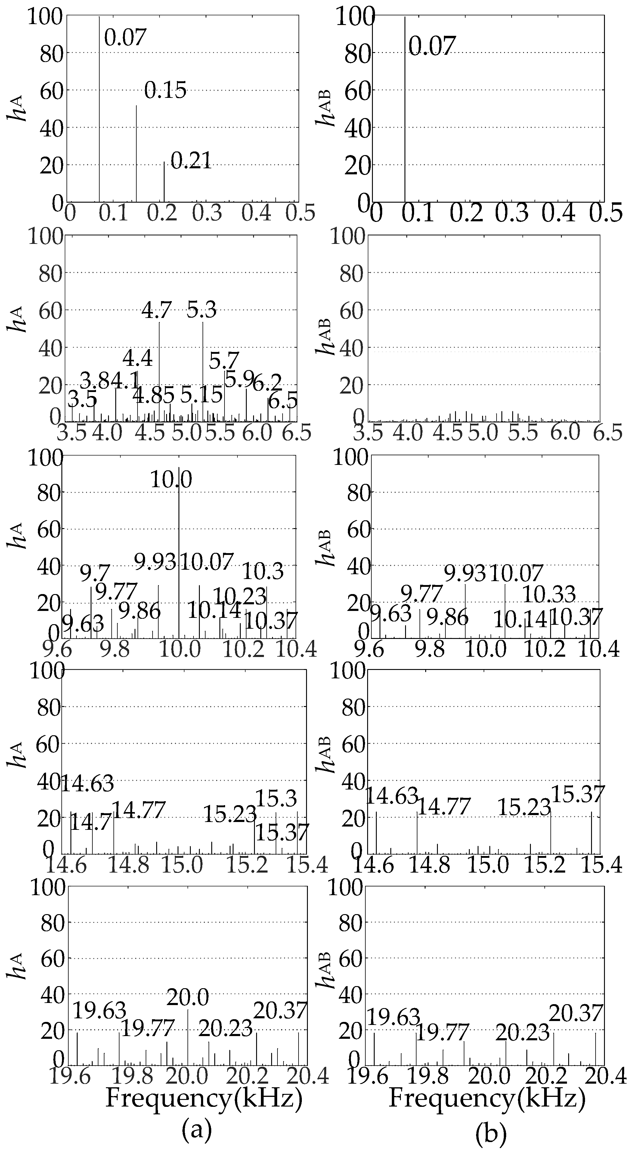It can be seen that the main harmonics are concentrated around the fundamental (k = 0) and 1 to 4 times of carrier frequency. Enlarge part of Figure 4 and mark the main harmonic frequency, as shown in Figure 5.

From Figure 5, it can be seen that the main components of low-frequency harmonics in output phase voltage are 3f_in and 3f_out. The amplitude of 3f_in is higher, which is up to 0.51 when m = 0.5. These two components belong to the common-mode voltage, so they are not contained in line voltage spectrum.

With respect to high-frequency harmonics, they cluster around an integer multiple of the carrier frequency and are symmetrical about the carrier frequency. Harmonics with high amplitudes in Figure 5 are listed in

Table 5. The main harmonic components in high-frequency bands.

f (kHz)	f	hA (%)
3.5/6.5	fc ± 30fin	9.69
3.8/6.2	fc ± 24fin	12.74
4.1/5.9	fc ± 18fin	17.66
4.4/5.6	fc ± 12fin	27.19
4.7/5.3	fc ± 6fin	53.29
4.85/5.15	fc ± 3fin	9.70
9.63/9.77/10.23/10.37	2fc ± fout ± 6fin	15.91
9.7/10.3	2fc ± 6fin	28.08
9.86/10.14	2fc ± 2fout	11.31
9.93/10.17	2fc ± fout	28.89
10.0	2fc	93.32
14.63/14.77/15.23/15.37	3fc ± fout ± 6fin	22.98
14.7/15.3	3fc ± 6fin	22.50
19.63//19.77/20.23/20.37	4fc ± fout ± 6fin	18.21
20.0	4fc	31.13

. The frequency expression of each harmonic in the table shows the relation between the frequency of main harmonics and the frequencies of input, output and carrier signals. Comparing the spectrum of phase voltage with line voltage, it is found that except the harmonics of 3f_in and 3f_out, there are other harmonic components which also belong to the common mode voltage, as marked gray in Table 5. The amplitude of 2f_c is the highest among all the harmonic components, up to 0.93 under the condition of m = 0.5, followed by the component of f_c ± 6f_in with the amplitude of 0.53. According to literature [18,19,20], high-frequency common-mode voltages are the main cause of bearing damage, winding fault, electromagnetic interference. The above analysis can accurately describe the amplitude of these common mode voltages, thus providing reference for the suppression of common mode voltage.

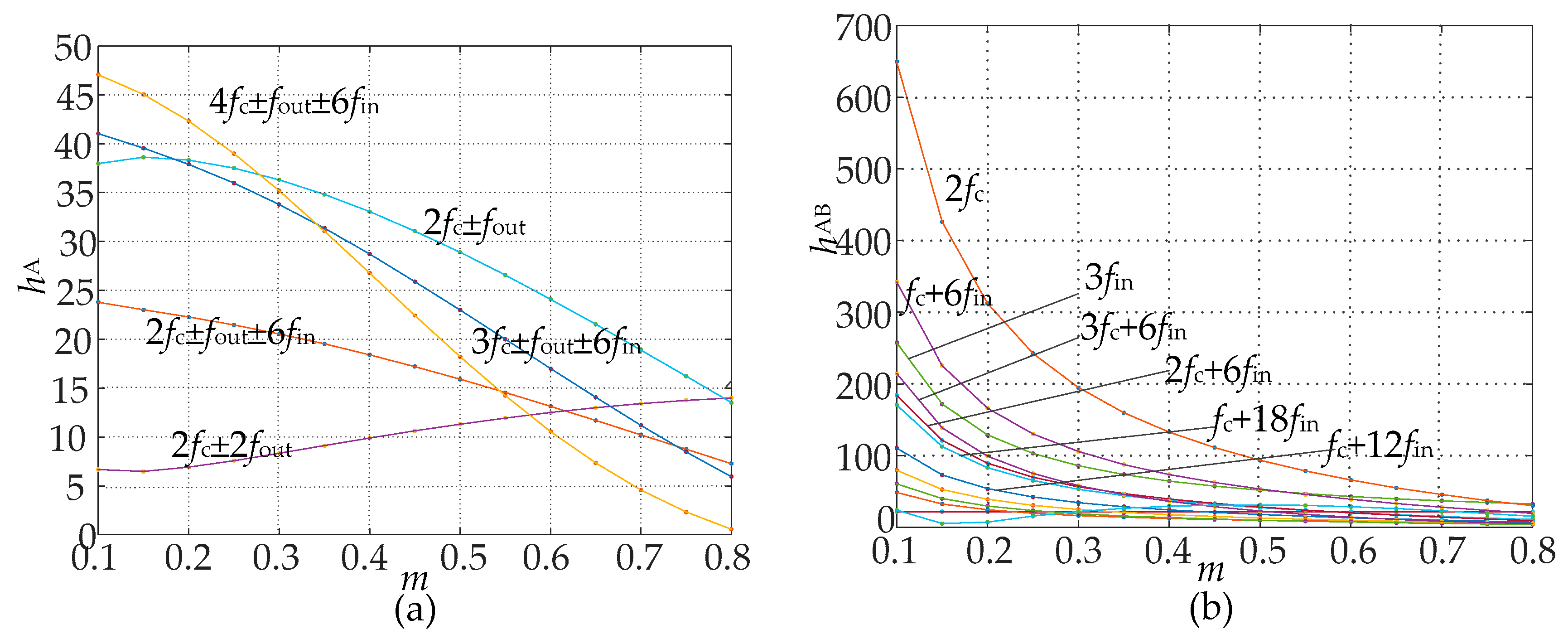
According to Equations (11) to (15), the amplitude of each harmonic is related to the voltage transmission ratio m. When m increases from 0.1 to 0.8, the relationship between amplitudes of main harmonics and m can be obtained, as shown in Figure 6. The harmonics in Figure 6a are components except for the common mode voltage in the output phase voltage. It can be seen that except the harmonic of 2f_c ± 2f_out most harmonics’ amplitudes decrease when m increase. The harmonics in Figure 6b are common mode components. When m ≤ 0.5, the amplitudes of 2f_c, f_c ± 6f_in, 3f_in and 3f_c ± 6f_in, are much higher than those of other harmonics. Besides, their amplitudes decrease rapidly with the increase of m. When m > 0.5, the amplitudes of harmonics in Figure 6b are gradually approaching, but still decrease with the increase of m.

From the above analysis, it can be seen that the amplitudes of high-frequency common mode components are much higher than those of other harmonics, especially when m is low. Besides, the harmonics’ amplitudes are affected by the value of m. Most harmonics’ amplitudes decrease gradually with the increase of m, but a few increase.

5. Comparative Analysis with FFT

The spectrums of the experimental waveforms cannot be obtained based on the triple Fourier series by the existing measurement techniques and analysis tools. FFT is usually used to deal with the experimental waveforms. Since it is very sensitive to the periodicity and frequency resolution of the waveforms, when the frequencies of input, output and carrier signals are all integers, and the time interval over which FFT is conducted as an integer multiple of the period of these three signals, the results obtained by the FFT analysis are accurate. However, when the values of these three frequencies are special (for example, the multiplicities of the three frequencies’ reciprocals are large or the three frequencies include non-integer), it is difficult to ensure that the time is an integer multiple of the carrier cycle, input and output voltage cycle. Under this condition, the harmonic spectrums obtained by FFT are not accurate. The following are the examples.

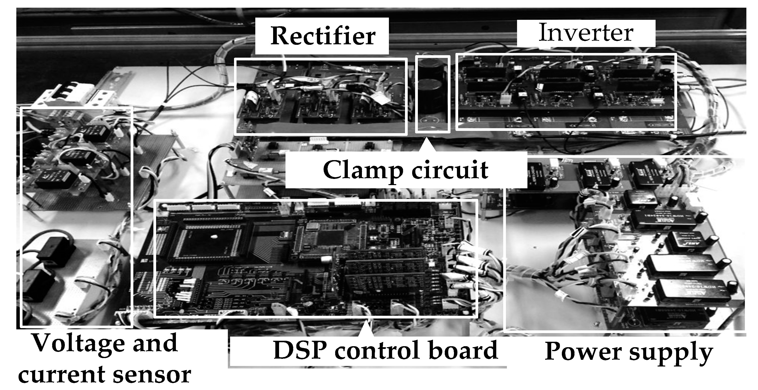
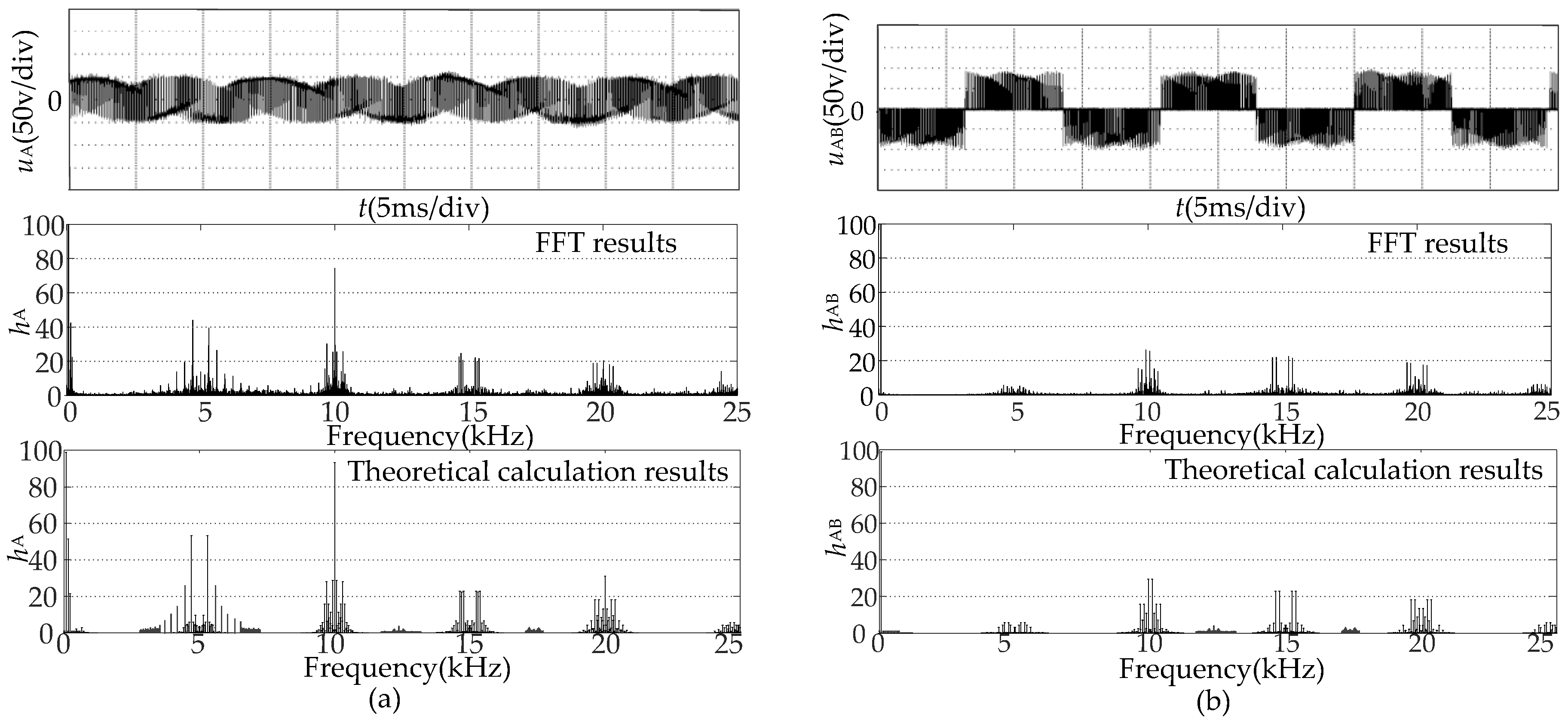
The spectrums obtained by FFT on the experimental waveforms of output voltage are compared with those analytical results based on the method proposed in this paper. Figure 7 shows the USMC experimental system. When the amplitude of input phase voltage is 42 V and the voltage transmission ratio m is 0.5, f_in = 50 Hz, f_out = 70 Hz, f_c = 5 kHz. The time domain waveforms of output voltage and their FFT results are shown in Figure 8, where Figure 8a denotes the waveform of phase voltage u_A and its FFT results and Figure 8b denotes the waveform of line voltage u_AB and its FFT results. The amplitudes of all the harmonic components in Figure 8 are the nominal value based on the fundamental amplitude. The FFT results in Figure 8 cuts out a section of the output voltage waveform for seven output voltage periods with a frequency resolution of 10 Hz. From the magnitudes of f_in, f_out, and f_c, the time corresponding to seven output voltage periods is an integer multiple of the carrier, input and output period so the FFT results are accurate. The main harmonic components in Figure 8 are listed in

Table 6. The main harmonic components in Figure 8.

FFT Results		Analytical Results
f (kHz)	hA (%)	f (kHz)	hA (%)
0.15	49.54	0.15	51.51
0.21	20.73	0.21	21.51
3.5/6.5	9.56	3.5/6.5	9.69
3.8/6.2	11.69	3.8/6.2	12.74
4.1/5.9	18.18	4.1/5.9	17.66
4.4/5.6	25.72	4.4/5.6	27.19
4.7/5.3	51.07	4.7/5.3	53.29
4.85/5.15	10.17	4.85/5.15	9.70
9.63/9.77/10.23/10.77	14.50	9.63/9.77/10.23/10.77	15.90
9.7/10.3	30.40	9.7/10.3	28.06
9.86/10.14	12.14	9.86/10.14	11.31
9.93/10.07	27.45	9.93/10.07	28.89
10.0	90.26	10.0	93.32
14.63/14.77/15.23/15.37	23.07	14.63/14.77/15.23/15.37	22.98
14.7/15.3	24.36	14.7/15.3	22.50
19.63/19.77/20.23/20.37	19.07	19.63/19.77/20.23/20.37	18.21
20.00	28.20	20.00	31.13

and compared with the results obtained from the analytical calculation. It can be seen that the frequencies of primary harmonics in Figure 8 are consistent with the analytical results but the amplitudes of them are slightly different. This is due to the existence of the switching dead-time, the conduction voltage drop of the switching device and the ripple of the input voltage at line side. The largest error between the measured spectrum and the theoretical results is only 3.06%.

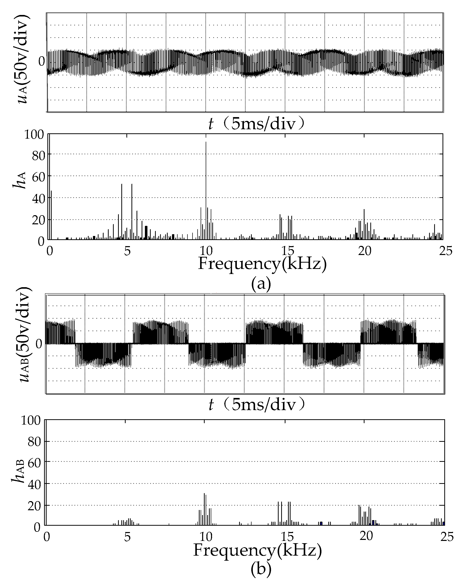
When f_in = 50 Hz, f_out = 70.5 Hz, f_c = 5 kHz, m = 0.5, the output voltage harmonic spectrums are shown in Figure 9. Under this condition, at least 141 periods of output waveform has to be intercepted to ensure the accuracy of FFT results. But the amount of data corresponding to 141 output periods is too large to be processed. The FFT results in Figure 9 intercepted a section of the output voltage waveform for seven output voltage periods with the frequency resolution of 10.07 Hz, it can be seen that there exist large errors between the FFT analysis and the analytical results. However, the analytic calculation method based on triple Fourier series in this paper is not affected by the magnitude of input, output and carrier frequencies. The analytical results can accurately determine the amplitudes and frequency of each harmonic component regardless of the magnitude of the three frequencies. In practical applications, the carrier frequency and the output frequency of USMC usually vary according to application requirements. Therefore, the method proposed in this paper has a wider scope of application than FFT.

6. Conclusions

In this paper, a theoretical calculation method based on three Fourier series is proposed for USMC under SVPWM. Taking input, output, and carrier frequencies into account, amplitudes and frequencies of harmonic components of output voltage are determined precisely for the first time. Including both the low-frequency harmonics and the high-frequency harmonic components, the relation between the frequencies of harmonic components and the frequencies of input, output and carrier signals can be determined. Through spectrum analysis in this paper, the following conclusions can be drawn:

• The frequencies of low-frequency harmonics are triple that of the input or output frequencies. The high-frequency harmonics are organized in sidebands and symmetrical about integer multiples of carrier frequency.
• The high-frequency common-mode components are kf_c + 6f_in, kf_c, etc., whose amplitudes are high. This feature is obvious, especially when the voltage transmission m is low.
• The harmonic amplitudes are affected by the value of m, and most of which decrease gradually with the increase of m, while a few decrease.