Article

Stationary-Frame Modeling of VSC Based on Current-Balancing Driven Internal Voltage Motion for Current Control Timescale Dynamic Analysis

State Key Laboratory of Advanced Electromagnetic Engineering Technology, Huazhong University of Science and Technology, Wuhan 430074, China
*
Author to whom correspondence should be addressed.
Energies 2018, 11(2), 374; https://doi.org/10.3390/en11020374
Submission received: 4 January 2018 / Revised: 29 January 2018 / Accepted: 31 January 2018 / Published: 6 February 2018

Abstract

:
High-frequency oscillations caused by voltage source converters (VSCs) are constantly emerging in power systems with the increasing penetration of renewable energies. VSC models in current control timescale play a pivotal role in the analysis of these oscillation issues. Conventional VSC models show few physical mechanisms of VSC dynamics during system oscillations. Hence, this paper proposes a VSC model from the viewpoint of its internal voltage (namely, VSC output voltage), which is driven by current balancing between the current reference and the feedback in a stationary frame. The proposed model can be used to study VSC dynamic characteristics in an intuitionistic physical way. Based on the proposed model, it is found that VSC current reference in a stationary frame varies with internal voltage dynamic due to the essence of active and reactive current control in a current control timescale. Additionally, in a stationary frame, the dynamic relation between internal voltage and error current embodies a generalized integrating characteristic with adaptable center frequency determined by a phase-locked loop, which guarantees the zero steady state error of VSC current control. Comparisons of simulations between the proposed model and a switch-based model validates the effectiveness of the proposed model.

1. Introduction

With the wide application of voltage source converters (VSCs) in power systems, the emerging oscillations caused by VSC control dynamics show diverse forms in multiple timescales [1,2,3]. In the current control timescale (CCTS) of VSCs, the unstable phenomena caused by VSCs, presenting as high-frequency oscillations, leads to financial loss for electricity companies [4]. Consequently, a system dynamics analysis in the current control timescale of a high VSC penetration system has received increasing attention from academic and industry scientists.
The VSC model is the foundation from which to study the dynamics issues of VSCs in current control timescale. Different kinds of VSC models have been proposed in published literature. The differential equation-based VSC model is usually used in modal analysis [5,6]. This kind of VSC model is deduced in the time domain and shows more mathematical detail than physical meanings. Early frequency-domain models of VSCs were deduced from the perspective of control theory and focused on the design of regulator parameters [7,8,9]. However, since the VSC and its external grid are modeled together, it is difficult to study VSC characteristics in such models. Therefore, the emerging impedance-based frequency domain model, in which VSC is modeled separately from the external grid, is proposed [10,11,12,13]. In this kind of model, as all of the control branches in VSCs are lumped into the equivalent impedance, the motion process of the inner key state in VSC is concealed, which limits the physical mechanism study of oscillations caused by VSCs. Therefore, it is necessary to propose a VSC model that is not only independent of its external grid but can also reflect the physical mechanism of the key state motion in VSC.
Generally, the output voltage of a grid-connected device is an important state to represent the motion of the device [14,15,16], as the voltage of each node is the most important index in the power system. In traditional synchronous generator (SG) modeling, the back electromotive force (EMF) is chosen to reflect the state of motion of the SG [15]. Recently, in the modeling of wind turbine generators (WTG), the equivalent output voltage is used to describe the device’s state of motion in an electromechanical timescale [16]. Furthermore, similar work was done in Reference [14] in which the output voltage of the VSC is used to reflect the dynamic behavior of the VSC in a DC voltage control timescale. However, in modeling a VSC in a current control timescale, there are few models that use the output voltage to reflect the state of motion in VSCs. In fact, in a current control timescale, it is easy to find that a system disturbance leads to an imbalance between the current reference and the feedback, and then the current balancing drives the motion of the internal voltage (namely, VSC output voltage) through the controller. Therefore, in a current control timescale, it is proper to model VSCs from the perspective of an internal voltage, which is driven by current balancing between current reference and feedback.
The VSC model can be deduced in a direct-quadrature (DQ) reference frame or stationary frame. Most existing VSC models are deduced in the DQ reference frame to avoid the periodically time-varying operation trajectories. However, as discussed in Reference [17], it is more difficult for DQ frame-based models to intuitively reflect the dynamic relations between three-phase quantities than models in a stationary frame. Moreover, for multi-machine system analysis in a current control timescale, the dynamic network model in a DQ frame is much more complicated than a stationary-frame model. Hence, in this paper, the proposed current-balancing driven internal voltage motion model of VSCs is carried out step by step in a stationary frame.
The rest of this paper is organized as follows: In Section 2, a brief description of a VSC current control system and some fundamental concepts are presented. Section 3 deduces, step by step, the current-balancing driven internal voltage motion model of VSCs. Then, the VSC dynamic characteristic analyses are shown in Section 4. Based on the proposed model, an interaction mechanism analysis between a VSC and a network is carried out in Section 5. Finally, several conclusions are drawn briefly in Section 6.

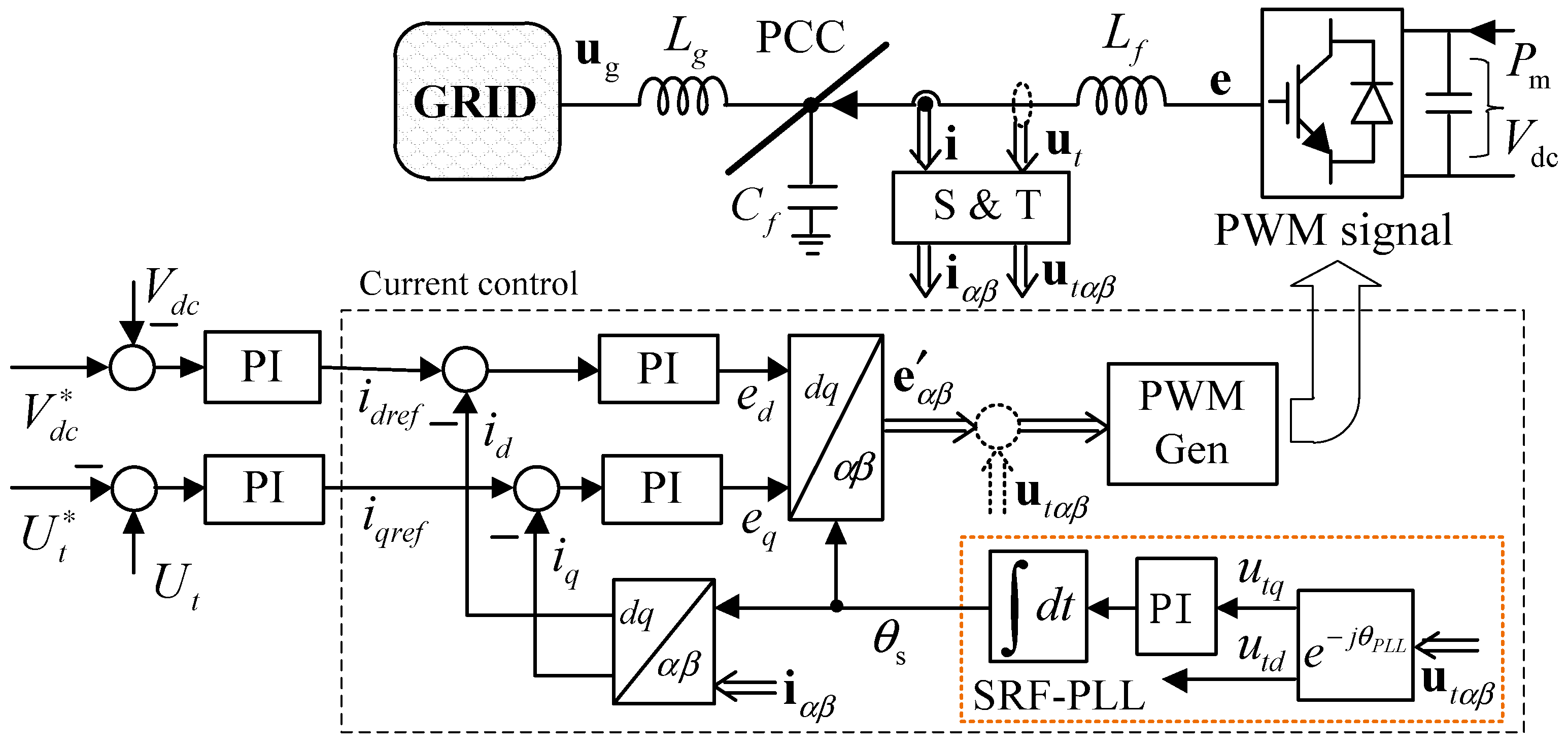
2. Description of VSC Current Control System and Fundamental Concept

The proportional plus integral (PI) regulator based on a synchronous reference frame phase-locked loop (SRF-PLL) is widely used in VSC current control. Figure 1 depicts a simplified diagram of VSC current control. The cross-decoupling items are neglected for simplification. The space vectors of current and voltage are denoted by boldface letters: for example, e for output voltage vector of VSC, ut for terminal voltage vector, ug for infinite bus voltage vector, and i for the current vector of VSC filter inductor. Signals in a SRF-PLL reference frame and stationary frame are denoted by subscript ‘dq’ and ‘αβ’. Those space vectors can be expressed by complex quantities [18,19]: for example, terminal voltage utαβ can be expressed as u + ju or Utej(ωt + ϴ) where Ut is the amplitude of the space vector. Additionally, it can be rewritten in real space vector form as [u, u]T. Unless otherwise stated, in this paper the bold non-italic letters represent real space vectors and transfer matrices and the bold italic letters represent complex vectors.

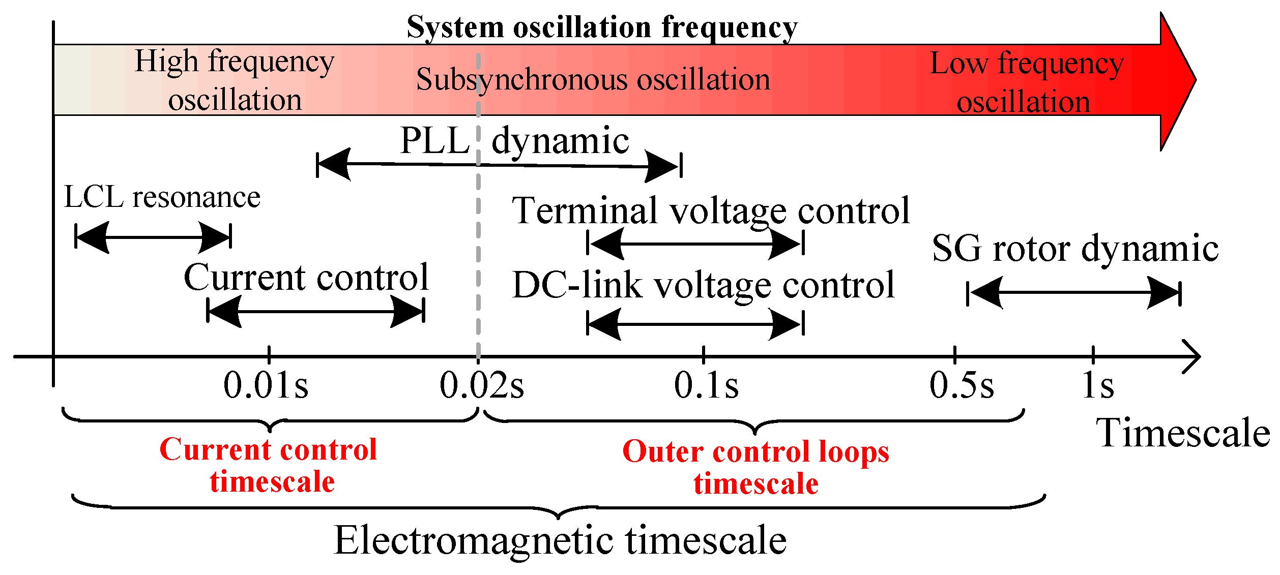
2.1. Definition of Current Control Timescale

Timescale decomposition is a useful tool for simplifying system dynamic analysis. According to the traditional timescale decomposition, the dynamics of VSC control loops belong to the electromagnetic timescale (less than 1 s). The current control loops have a minimum response time constant (less than 20 ms) among VSC control loops [4]. The outer control loops, such as DC-link voltage control and terminal voltage control, have a much slower dynamic (about 20 ms to 1 s) [14]. The phase-locked loop’s dynamic response time constant is between those of the outer loops and current control loops. The relative relations of different VSC control loops and their response time constants are shown in Figure 2. To study the high frequency oscillations caused by VSCs, this paper focuses mainly on dynamics less than 20 ms, and defines it as current control timescale. Therefore, the outer control loops are ignored in the modeling, except the SRF-PLL.

2.2. The Internal Voltage of VSCs in Current Control Timescale

For power system operation, the voltage of each node in a grid is an important index to evaluate the system’s state. The grid node voltage is mainly determined by the output voltage of each grid-connected device—for example, the back EMF in SG, the output voltage of VSC in WTGs, and so on. The dynamics of each device’s output voltage has significant impact on power system dynamics. In this paper, the device output voltage is defined as the internal voltage since its dynamic is only determined by the device itself. For the VSC, the AC side inverter voltage is defined as its internal voltage.
As mentioned above, the dynamic of the device’s internal voltage has an important impact on system dynamics. In addition, the dynamics of the internal voltage is determined by the VSC inner control process. Thus, in order to intuitively reflect the influence of VSC on the system dynamics, this paper models VSC from the perspective of the internal voltage, in which the internal voltage is used as the output interface of the proposed VSC model, and the current reference and feedback are used as the model input interface. From this perspective, it is possible to find that the dynamics of the VSC’s internal voltage in the current control timescale is physically determined by balancing between current reference and feedback current. Furthermore, current balancing will be impacted by the PLL through coordinate transformations. Based on the considerations above, a current-balancing driven internal voltage motion model of VSC is proposed in this paper.

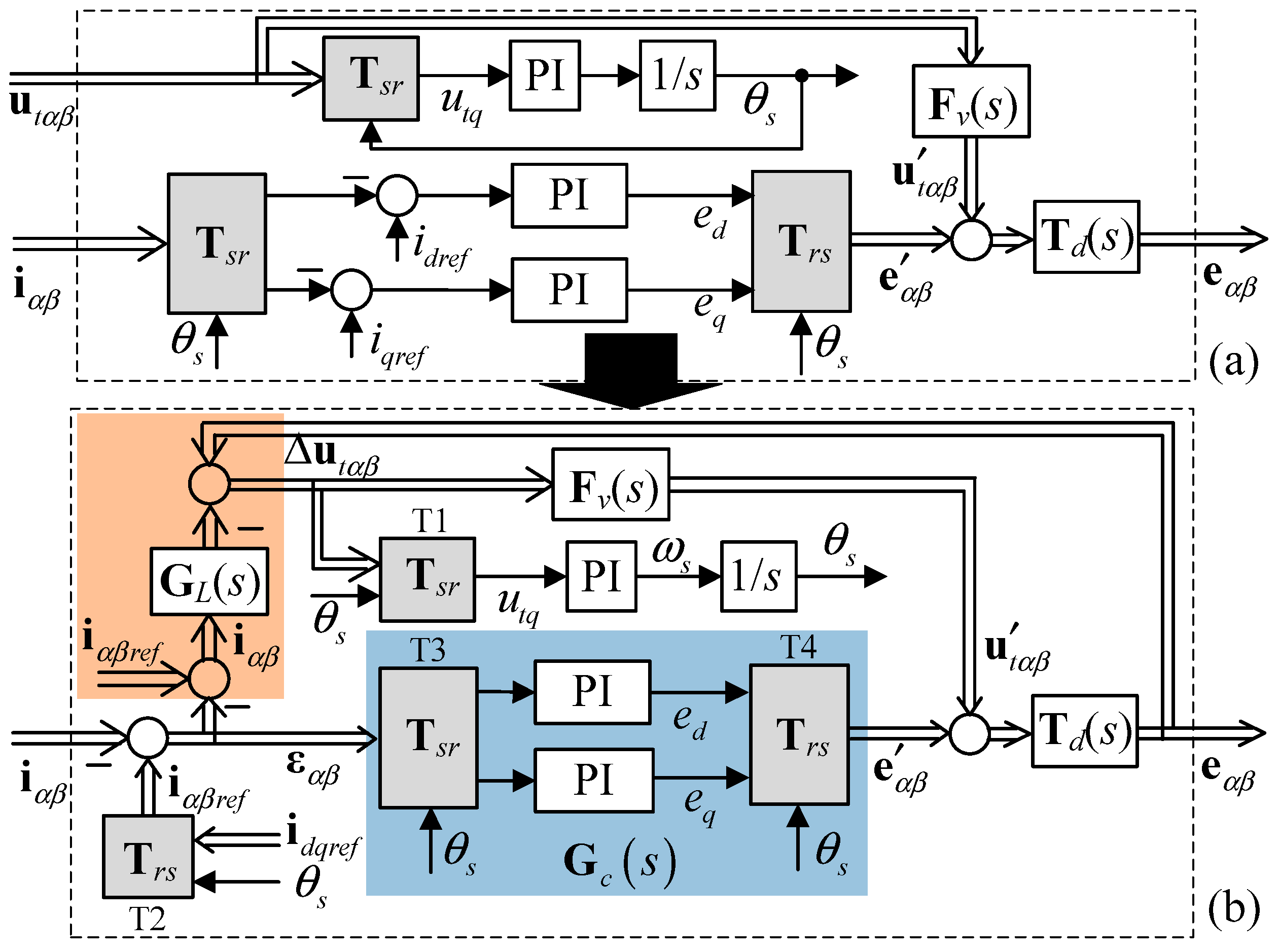
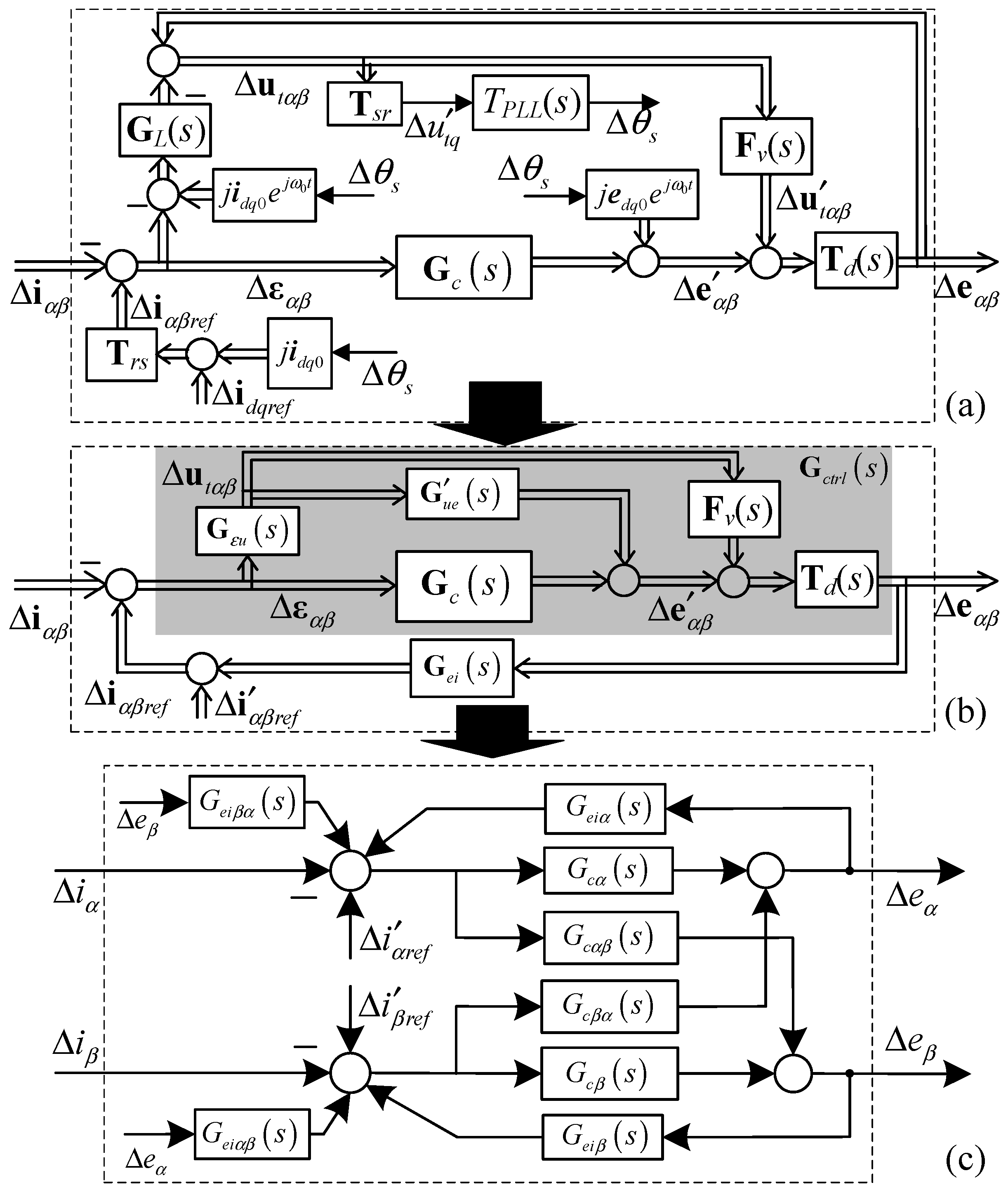
3. Current-Balancing Driven Internal Voltage Motion Model of VSCs in Stationary Frame

In this section, the current-balancing driven internal voltage motion model with the consideration of SRF-PLL is deduced step by step by block diagram in a stationary frame. Comparisons of simulations between the proposed model and a switch component-based model are used to verify the proposed model.

3.1. The Modeling of VSCs in Stationary Frame

According to the current control diagram shown in Figure 1, it is possible to obtain a diagram description of a VSC in Figure 3a. Tsr and Trs in Figure 3a represent the coordinate transformation with the mathematical form as
T s r = T r s 1 = [ cos θ sin θ sin θ cos θ ]
In Figure 3, the PIs are the proportional-integral regulators for current control and SRF-PLL. The PI parameters for current control are denoted by kpc and kic, while the PI parameters for PLL are denoted by kps and kis. The transfer function matrix Fv(s) is used to simulate the effect of the sample and filter on the voltage feedforward pathway and can be written as:
F v ( s ) = [ f v ( s ) 0 0 f v ( s ) ]
where fv(s) = afv/(s + afv), and afv is the cutoff angular frequency. Td(s) is used to simulate the time delay effect caused by sampling, digital control, PWM implementation, and so on, and is
T d ( s ) = [ f i ( s ) 0 0 f i ( s ) ] e 1.5 T s s
where fi(s) = afi/(s + afi), and afi is the cutoff angular frequency. Ts is the sampling period, which is set as 2.1 kHz.
Replacement of the terminal voltage by current and internal voltage: As mentioned above, the reference and feedback currents are chosen as the input interface of the proposed model in this paper. However, the input of the PLL is terminal voltage utαβ. In order to unify the input interface of the model, it is necessary to replace utαβ by another quantity in VSC. In fact, utαβ can be replaced by iαβ and e based on their mathematical relations of filter inductor on the AC side:
u t α β = e α β [ s L f 0 0 s L f ] G L ( s ) i α β
Furthermore, iαβ equals the difference of iαβref and εαβ. Thus, it is possible to convert the block diagram shown in Figure 3a into an equivalent form, shown in Figure 3b.
The self-adaption resonant characteristic of SRF-PLL-based dual PI control in a stationary frame: The blue shadow area in Figure 3b presents the equivalent control diagram of SRF-PLL-based dual PI regulators in a stationary frame. According to the control diagram, the regulators’ outputs in the stationary frame can be written as the sum of the output of the proportional part and the integral part, which can be expressed as follows:
[ e α e β ] = T r s k p c I 2 × 2 T s r [ ε α ε β ] + [ x α x β ]
where [xα, xβ]T is the output of the integral regulator in a stationary frame, and can be obtained by the state-space equation as:
[ x ˙ α x ˙ β ] = [ 0 ω s ( t ) ω s ( t ) 0 ] [ x α x β ] + 1 k i c [ 1 0 0 1 ] [ ε α ε β ]
where ωs(t) is the differential of θs as shown in Figure 3b. Thus, the SRF-PLL-based dual PI regulator is a time-varying system in a stationary frame if the dynamic of PLL is considered.
If the output angular velocity ωs(t) of PLL is assumed as constant, it is possible to obtain the transfer function between error current and internal voltage from Equations (5) and (6) as follows:
[ e α ( s ) e β ( s ) ] = { [ k p c 0 0 k p c ] + k i c s 2 + ω s 0 2 [ s ω s 0 ω s 0 s ] } G c ( s ) [ ε α ε β ]
From Equation (7), the integral part of the PLL-based dual PI regulators acts as a generalized integrating characteristic with its center frequency at ωs0 in a stationary frame. However, in a practical power system, the system’s frequency is a slowly varying function of time. The SRF-PLL in VSCs follows the system frequency. Hence, the characteristic of SRF-PLL-based dual PI regulators in a stationary frame can be viewed as an adaptable resonant controller with its center frequency ωs(t) regulated by PLL.
Linearization of coordinate transformations: The model shown in Figure 3b is still a nonlinear model for the existence of the coordinate transformations. These transformations are nonlinear for the time-varying angular frequency caused by the PLL dynamic [17]. Therefore, the linearization of coordinate transformations is the foundation for obtaining the small-signal VSC model. To overcome this difficulty, the harmonic linearization is introduced into VSC modeling [20,21]. This paper shows a different way to obtain the linearized VSC model in a stationary frame. In fact, the coordinate transformation can be easily linearized in polar coordinates since the steady value of vector magnitude and angular frequency are DC variables. The detail derivation process of the coordinate transformation linearization is shown in the Appendix A.
By applying the linearization process in T1, T2, T3, and T4, it is possible to get the corresponding linearized transformation as follows:
[ Δ u t d Δ u t q ] [ 0 Δ θ s U t 0 ] + T s r [ Δ u t α Δ u t β ]
[ Δ i α r e f Δ i β r e f ] T r s [ i q 0 Δ θ s i d 0 Δ θ s ]
[ Δ ε d Δ ε q ] T s r [ Δ ε α Δ ε β ]
[ Δ e α Δ e β ] T r s { [ e q 0 Δ θ s e d 0 Δ θ s ] + [ Δ e d Δ e q ] }
According to the SRF-PLL diagram shown in Figure 1, Δθs in Equations (8), (9), and (11) can be obtained as:
Δ θ s = k p s s + k i s s 2 + u t d 0 k p s s + u t d 0 k i s T P L L ( s ) Δ u t q .
After linearization of the coordinate transformations, it is possible to convert Figure 3b into the linear model shown in Figure 4a. However, the system in Figure 4a is still a linear periodically time-varying system in a stationary frame for the DQ asymmetry introduced by the branch of PLL. Hence, it is difficult to obtain the corresponding frequency domain model in a stationary frame.
In order to deduce the frequency model in a stationary frame, the system in Figure 4a should be simplified into a DQ symmetric one. According to Reference [22], an unsymmetrical matrix can be equivalently converted into two symmetrical matrices. Hence, by substituting Equation (12) into Equations (9) and (11), the transformations can be rewritten as
[ Δ i α r e f Δ i β r e f ] T r s { G u i + ( s ) [ Δ u t d Δ u t d q ] + G u i ( s ) [ Δ u t d Δ u t d q ] }
[ Δ e α Δ e β ] T r s { G u e + ( s ) [ Δ u t d Δ u t q ] + G u e ( s ) [ Δ u t d Δ u t q ] + [ Δ e d Δ e q ] }
where Gui+(s), Gui(s), Gue+(s), and Gue(s) are transfer function matrices and shown in the Appendix B.
If the components introduced by Gui(s) and Gue(s) in (13) and (14) are both neglected, the system shown in Figure 4a can be converted into a DQ symmetric one. Hence, it becomes possible to obtain the system stationary-frame model as shown in Figure 4b. Note that Gui+(s) and Gue+(s) are denoted to descript the dynamic relations in a DQ frame, and G′ui(s) and G′ue(s) are denoted to replace them in the stationary frame. The illustration of Figure 4b is shown as follows:
The dynamic relation between error current and terminal voltage: According to the diagram in Figure 4a, the terminal voltage Δutαβ can be calculated by the error current and internal voltage. Furthermore, it is able to simplify the calculation of terminal voltage Δutαβ through error current by
G ε u ( s ) = [ G c ( s ) T d ( s ) + G L ( s ) ] · [ I 2 × 2 + G L ( s ) G u i ( s ) T d ( s ) ( G u e ( s ) + F v ( s ) ) ] 1
The dynamic relation between internal voltage and current reference: In Figure 4a, the transformation between the DQ current reference and the stationary frame current reference is affected by the PLL dynamic through Δθs. In addition, the terminal voltage, which is the input of PLL, is influenced by the internal voltage Δeαβ. Therefore, in Figure 4b, the dynamic relation between the internal voltage Δeαβ and the stationary frame current reference is highlighted by Gei(s). This is an important dynamic characteristic that relates to the active and reactive current control. More discussions will be presented in the following text. The Gei(s) can be calculated by:
G e i ( s ) = G u i ( s ) · G ε u ( s ) G c t r l 1 ( s )
The dynamic relation between internal voltage and error current: The internal voltage in VSC is directly driven by the imbalance between current reference and feedback. Thus, the dynamic relation between internal voltage and error current shows the control behavior of VSC in a stationary frame. This dynamic relation is shown in Figure 4b by Gctrl(s), which is the synthetic transfer function matrix of the dynamic relations in the shadow area. The Gctrl(s) can be obtained by:
G c t r l ( s ) = T d ( s ) [ G c ( s ) + ( G u e ( s ) + F v ( s ) ) G ε u ( s ) ]
In fact, Gctrl(s) in Figure 4b clearly presents the influence of the current PI regulator, the PLL, and the voltage feedforward on the internal voltage through three branches. Furthermore, it shows that there is a similar influence of PLL and voltage feedforward on internal voltage; that is, both of them can impact internal voltage through the feedforward pathway. In Figure 4c, the model is presented in the form of transfer functions. Geiα(s), Geiβα(s), Geiαβ(s), and Geiβ(s) are the elements of the transfer matrix Gei(s) in (16). G(s), Gcβα(s), Gcαβ(s) and G(s) are the elements of the transfer matrix Gctrl(s).
From what has been deduced above, the current-balancing driven internal voltage motion model of VSC in current control timescale has been obtained in Figure 4c. It is worth noting that it is possible to obtain the impedance-based VSC model in a stationary frame through the rearrangement of the proposed model. In order to have a more insightful view of VSC, the VSC dynamic characteristic will be studied in the next section.

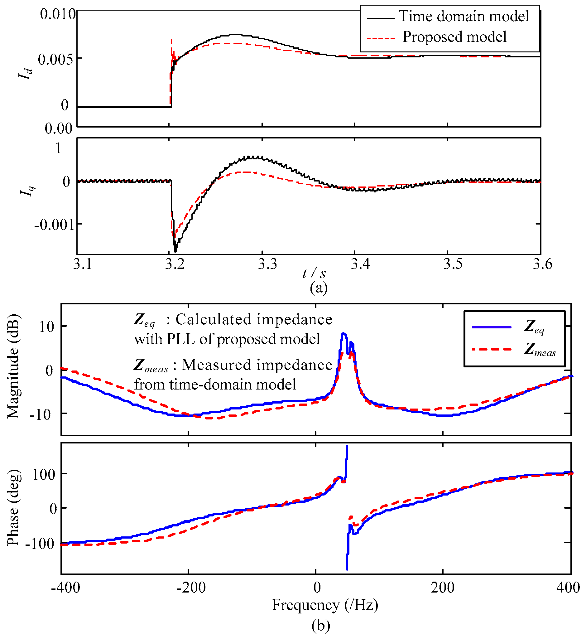
3.2. Verification of the Proposed Model

To verify the correctness of the proposed VSC model, a comparison of a step response and VSC equivalent impedance between a switch-based time-domain VSC model and the proposed model was carried out. The main parameters used in the two models are presented in Table 1. In time-domain simulations, a step disturbance in the current reference appears at 3.2 s in the two different models. In order to make the comparison more observable, all the waves are converted into a rotating DQ reference with a constant angular velocity. The step responses of current Id and Iq are shown in Figure 5a. It can be seen that the dynamic response of the proposed VSC model coincides with the time-domain model, which verifies the correctness of the model proposed in this paper. The differences between the two models are caused by the Insulated Gate Bipolar Transistor (IGBT) dynamics in the time domain simulation and simplification of the linearization on coordinate transformation in the proposed model. The difference of the fast and short transient at 3.2 s between the two models is caused by the parasitic resistance of passive components in the network. Figure 5b shows the VSC impedance comparison between the two models. The blue line presents the calculated impedance of the proposed VSC model and the red-dashed line presents the measured impedance of the time-domain model. The impedance measure of the time-domain model is realized by frequency scans in the time-domain simulations. Both comparisons between the two kinds of models show that the proposed model can reflect the primary characteristics of a VSC in a stationary frame.

4. VSC Dynamic Characteristic Analysis in Current Control Timescale

The characteristics of grid-connected devices affect system dynamic behavior. This section discusses the dynamic characteristic of a VSC in stationary frame from a physical viewpoint. Firstly, the characteristics of a variable current reference in the proposed model are concluded. Then, the VSC control characteristics in a stationary frame are discussed and the influence of PLL on VSC is presented.

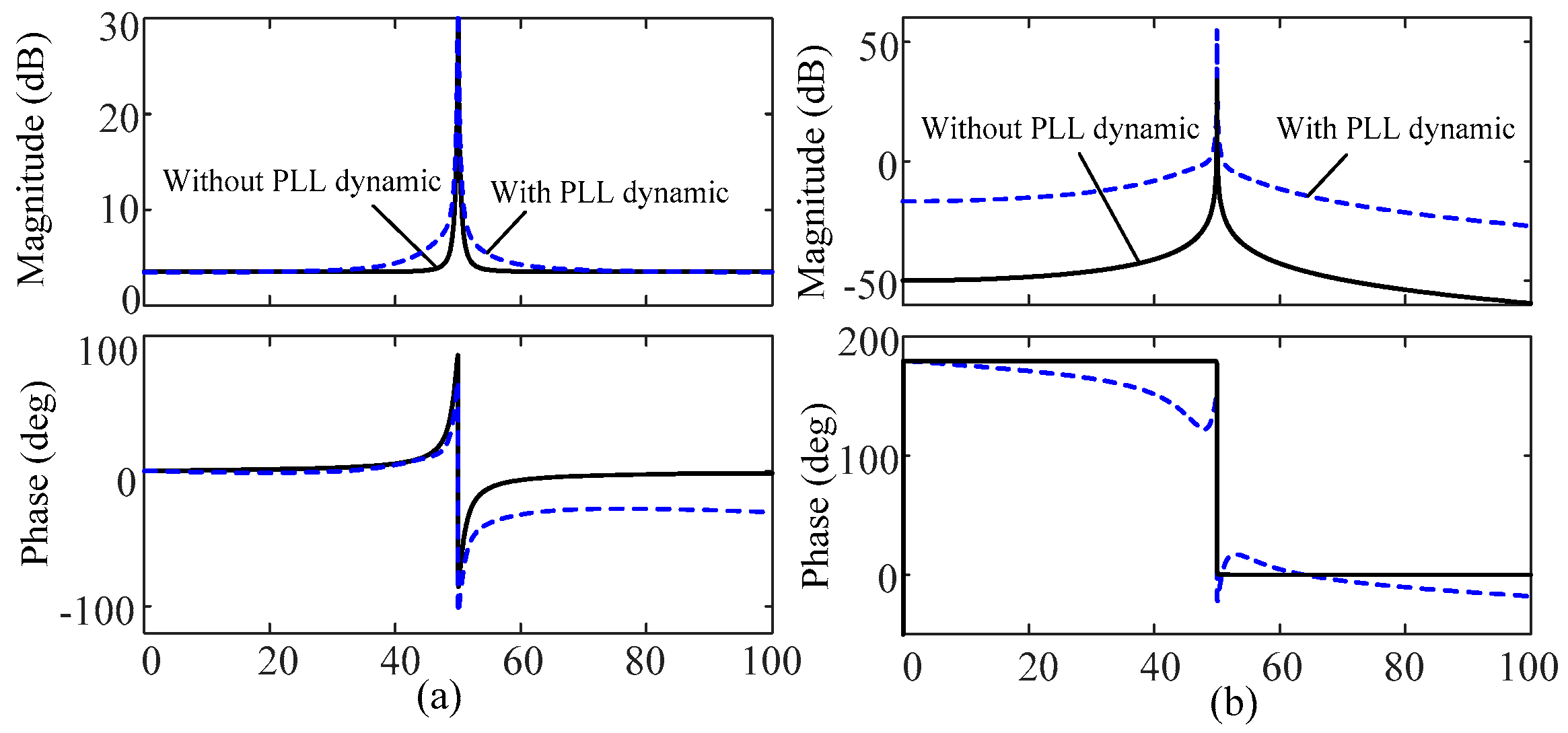
4.1. The VSC Characteristic of Variable Current References in Stationary Frame

The current reference is a key quantity in VSC current control. Generally, the current reference is treated as a constant in most cases of VSC current control analyses. However, since the current references are generated by the outer control loops in the PLL reference frame, the current references will become variable quantities if they are converted into a stationary frame. This is because the stationary-frame references are calculated by the DQ current reference and coordinate transformation, while the coordinate transformation introduces the variable components into the stationary-frame reference. Naturally, the variation of current references will be impacted by the PLL dynamic through the coordinate transformation. The characteristics of the variable current references affect VSC dynamic behavior greatly during a system disturbance. The proposed model in Figure 4c clearly shows this characteristic through the block diagram.
In order to present the dynamic relations of Gei(s) intuitively, the time-domain simulation response of current reference and internal voltage in a stationary frame are shown in Figure 6. The time-domain simulation is based on the system in Figure 1 with its parameters shown in Table 1. The simulation results show that the current reference will change with internal voltage in the same tendency. There is only a short time delay between the two waves, which is caused by the phase shifts of Gei(s).
Due to the characteristic of variable current reference, the increased internal voltage leads to increasing current reference, which then increases the error current, which may lead to a further increase of the internal voltage. In other words, the characteristic of the variable current reference may introduce negative damping in VSCs during system dynamic processing. This dynamic characteristic of VSCs may deteriorate system stability.

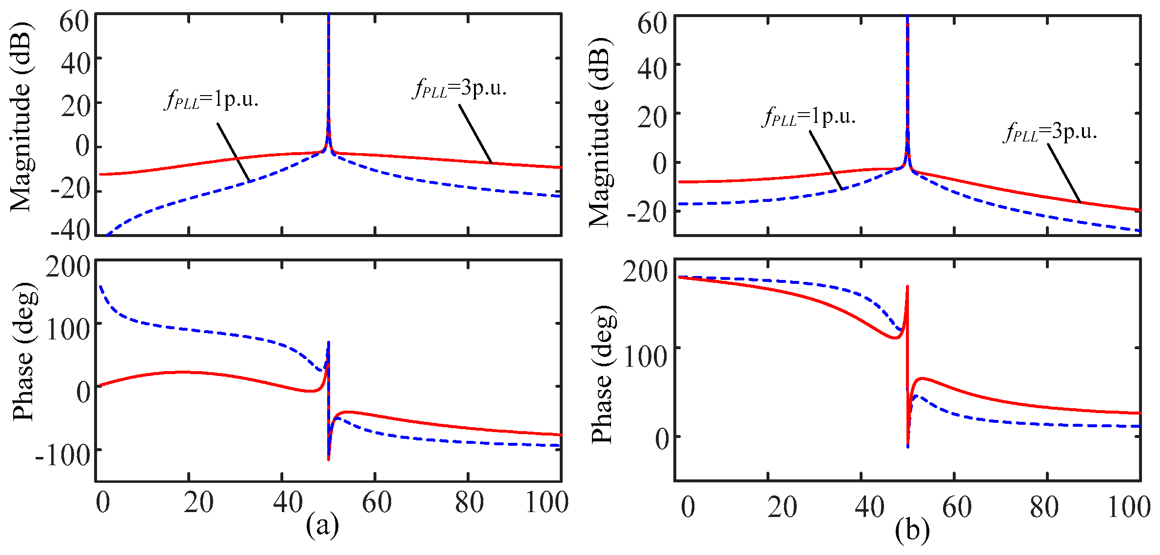
4.2. Control Characteristic of the VSC in Stationary Frame

In current control timescale, the current control loop in a grid-connected VSC can be viewed as a typical control system design. The VSC control characteristic that reflects the dynamic relation between error current and internal voltage is important to the dynamic response of the current control loop. In most cases, the VSC control characteristic is treated as the characteristic of the PI regulator in a DQ reference frame. According to the conclusion in Reference [23], the VSC control characteristic can be described by a proportional resonant controller in a stationary frame when the dynamic of PLL is ignored. However, there is no literature that discusses the VSC stationary frame control characteristic in consideration of the PLL dynamic, which makes the following work necessary.
According to the frequency model shown in Figure 4c, the VSC control characteristic can be intuitively reflected by the transfer function matrix Gctrl(s) between the error current and internal voltage. In Figure 7, the Bode plots of the diagonal and off-diagonal elements in Gctrl(s) are presented; the impact of the terminal voltage feedforward is ignored in the plots for simplification. By analyzing the Bode plots in Figure 7, it is possible to find the impact of the PLL dynamic on the VSC control characteristic. It is obvious that Gctrl(s) acts as a PR controller if the PLL dynamic is ignored, and the existence of the PLL dynamic can broaden the bandwidths centered at the fundamental frequency. Additionally, the coupling between different axes in an αβ stationary frame will be increased by the PLL dynamic, which is reflected in the Bode plot of the off-diagonal in Figure 7b. In summary, the existence of the resonance centered at the fundamental frequency in Gctrl(s) makes the VSC able to realize the zero steady state error current control in a stationary frame. This control characteristic is similar to the generalized integrating characteristic as discussed in Reference [23].
A further in-depth perspective of the PLL’s influence on the VSC control characteristic can be discussed based on the diagram shown in Figure 4b. The Gc(s) presents the stationary frame PR regulator, which relates to the PI regulator in the PLL reference frame. In addition, the existence of the PLL dynamic introduces a branch, which is formed by the transfer function matrix Gεu(s) and G′ue(s), in parallel with Gc(s) in Figure 4b. The Bode plots of the diagonal and off-diagonal elements in Gεu(s)G′ue(s) are shown in Figure 8. It shows that Gεu(s)G′ue(s) also has a resonance point at the fundamental frequency. Increasing the PLL bandwidth leads to the increase of Gεu(s)G′ue(s) in a wide frequency band, which may increase the gain of Gctrl(s) and affects the control system dynamic. Furthermore, by comparing Figure 7b and Figure 8b, it is possible to find the reason why the coupling between the α and β axes in Gctrl(s) increased in consideration of the PLL dynamic. This is caused by the high gain of the off-diagonal element in Gεu(s)G′ue(s).
Note that the above conclusions are obtained based on the linearized model. For the nonlinear model shown in Figure 3b, the resonance frequency of the VSC controller in a stationary frame is determined by the PLL operation point, which is affected by the external grid state. In other words, VSC shows an adaptable generalized integrating characteristic with its center frequency determined by PLL.

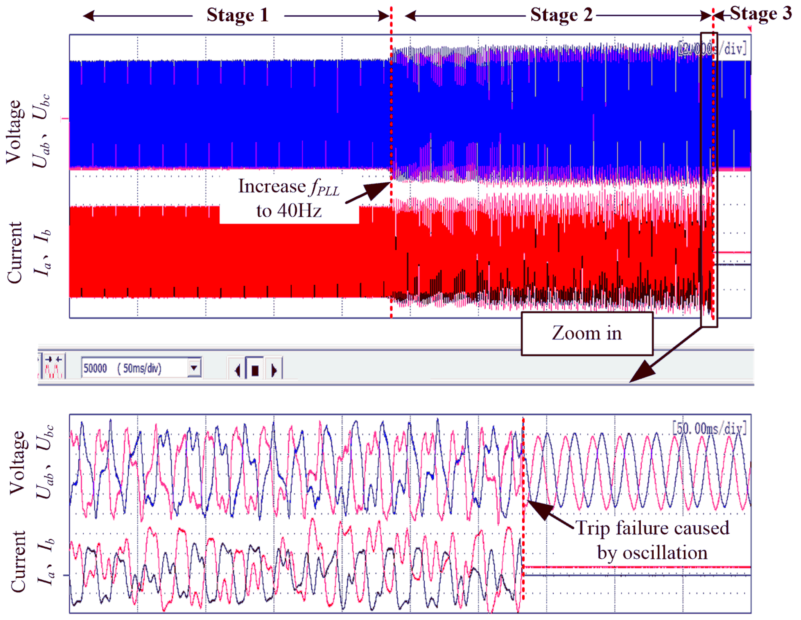
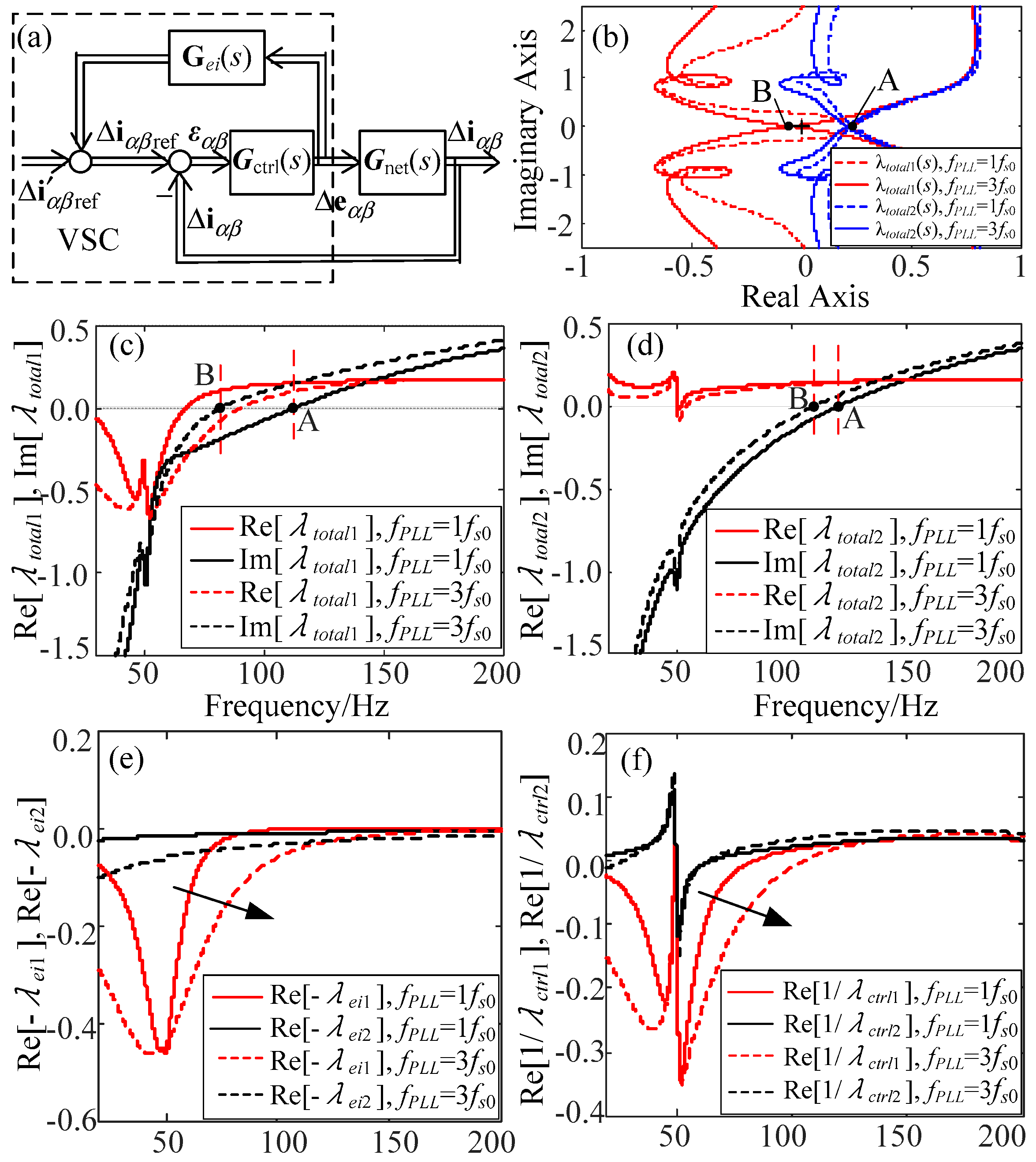
5. Application of the Proposed Model in Stability Analyses of a Grid-Connected VSC

In this section, the stability of the system shown in Figure 1 is elaborated upon as an application example of the proposed model. The interaction between a VSC and an external grid is studied.
In system oscillation caused by the interaction between VSC control strategies and the network, the VSC dynamic characteristics studied above can be used to indicate the impact of VSCs on system stability. By combining the characteristics of both the VSC and the network, it is possible to evaluate system stability.
The system shown in Figure 1 can be described by the block diagram shown in Figure 9a. The VSC is described by the proposed model and the network is represented by the transfer function matrix Gnet(s) as:
G n e t ( s ) = [ G g ( s ) 0 0 G g ( s ) ]
where Gg(s) is:
G g ( s ) = s L f ( s L g + 1 / ( s C f ) + R d ) s 2 L f 2 ( s L g + 1 / ( s C f ) + R d ) + s L g ( 1 / ( s C f ) + R d )
According to Figure 9a, it is possible to obtain the dynamic relation of current reference Δi′αβref and internal voltage Δeαβ as:
Δ e α β = [ G n e t ( s ) G e i ( s ) + G c t r l 1 ( s ) G t o t a l ( s ) ] 1 Δ i α β r e f
Therefore, the system stability can be evaluated by the inverse of Gtotal(s). Furthermore, according to the generalized Nyquist criterion of matrix transfer function [24], the system stability evaluation can be simplified to the analysis of the characteristic loci of Gtotal(s). The characteristic loci can be calculated by:
λ t o t a l 1 , 2 ( s ) = g 11 ( s ) + g 22 ( s ) ± [ g 11 ( s ) g 22 ( s ) ] 2 + 4 g 12 ( s ) g 21 ( s ) 2
where g11(s) and g22(s) are the diagonal elements in Gtotal(s); g12(s) and g21(s) are the off-diagonal elements in Gtotal(s).
The Nyquist curves of the characteristic loci in Gtotal(s) are shown in Figure 9b with the change of PLL bandwidth from 1 fs0 to 3 fs0. fs0 is the bandwidth of PLL that is calculated by initial parameters. Since Gtotal(s) has no Smith–McMillan pole on the right-half plane, the system will be stable if there is no encirclement of the characteristic loci around the original point. In Figure 9b, it is obvious that the cross-point of λtotal1(s) on the real axis changes from A to B when the PLL bandwidth is increased, which indicates that the system will become unstable. This conclusion coincides with published literature [25,26].
In fact, the encirclement of the Nyquist curves at the original point in Figure 9b can be recognized by the real part of the curves when its imaginary part is zero. Therefore, the system stability criterion can also be simplified into the formula shown in Equation (22) where λtotal(jω), λctrl(jω), λei(jω), and λnet(jω) are the characteristic loci of Gtotal(jω), Gctrl(jω), Gei(jω) and Gnet(jω). ‘Im[ ]’ and ‘Re[ ]’ denote the imaginary and real parts of the complex variable. Based on Equation (22), Figure 9c,d indicates the system stability more directly. In Figure 9c, it is clear that Re[λtotal1(jω)] will become negative when Im[λtotal1(jω)] crosses the abscissa axis at point B, which indicates the instability of the system. The plots in Figure 9c indicate that the unstable frequency band is close to but higher than the fundamental frequency. Note that it is impossible to find the potential oscillation frequency in a stationary frame by the DQ frame-based VSC model. This is a comparative advantage of the proposed model in this paper over the DQ frame-based VSC model.
Furthermore, as shown in Equation (22), the characteristic loci of Gtotal(jω) can be calculated by the characteristic loci of Gctrl(jω), Gei(jω), and Gnet(jω). Thus, based on the proposed model, the impacts of Gctrl(jω) and Gei(jω) on system stability can be studied directly, which shows insight into the physical mechanism of VSC on system dynamic stability. Figure 9e,f shows the real part of -λei(jω) and 1/λctrl(jω). It is obvious that the increasing PLL bandwidth will decrease the Re[−λei1(jω)] and Re[1/λctrl1(jω)]. This will cause the system stability to deteriorate.
{ Im [ λ t o t a l ( j ω ) ] = 0 , Re [ λ t o t a l ( j ω ) ] > 0 Stable Im [ λ t o t a l ( j ω ) ] = 0 , Re [ λ t o t a l ( j ω ) ] = 0 Ctritically   Stable Im [ λ t o t a l ( j ω ) ] = 0 , Re [ λ t o t a l ( j ω ) ] < 0 Unstable λ t o t a l ( j ω ) = 1 λ c t r l ( j ω ) λ e i ( j ω ) + λ n e t ( j ω )
To verify the analysis results above, a 10 kW experiment platform of grid-connected VSC based on dSPACE was implemented and the same per unit value parameters used in the analyses were assigned in the experiment system. The influences of SRF-PLL bandwidth on current control stability were checked. The experimental results of VSC attached to a weak grid are shown in Figure 10. There are three stages in the experiment:
  • Stage 1: the system is in a state of stable operation with 10 kW of active power output;
  • Stage 2: the PLL bandwidth is changed to 40 Hz; and
  • Stage 3: a trip failure caused by oscillations leads to disconnection of the VSC.
The theoretical analysis results in Figure 9 show that the system will become unstable in Stage 2; the experimental results coincide with the theoretical analysis. In Stage 3, the waves show that the VSC is disconnected from the grid, caused by the oscillation.

6. Conclusions

This paper proposed a VSC dynamic model that is established from the perspective of its internal voltage for power system dynamic analysis in current control timescale. From the proposed model, it is possible to find the physical essence of a VSC dynamic in the current control timescale during a system disturbance, which can be described as the motion of internal voltage driven by current balancing between the current reference and feedback in a stationary frame. Based on the proposed VSC model, the VSC dynamic characteristics can be studied from two aspects: (1) the VSC variable current reference characteristic, which is essentially caused by active and reactive current control; and (2) the adaptable generalized integrating characteristic of VSC with its center frequency determined by the PLL in stationary frame. Furthermore, the impact of PLL bandwidth on VSC dynamic characteristic is discussed. Moreover, the application of the proposed model in stability analysis of a single VSC infinite bus system shows the mechanism of the control interaction between the VSC and the network in current control timescale. The experimental prototype-based tests verify the correctness of analyses.

Acknowledgments

The work presented in this paper was fully supported by the grant from the National Key Research and Development Program of China (2016YFB0900104) and the grant from the Basic Research Project of Qinghai Province of China (2016-ZJ-767). The authors would like to thank Xiaojie Zhang and Lei Shang from SEEE, Huazhong University of Science and Technology, for their help on the experiments.

Author Contributions

Yabing Yan, Xiaoming Yuan and Jiabing Hu propose the main idea of the paper. Yabing Yan also implements the mathematical derivations, simulation analyses and experimental verification. The paper is written by Yabing Yan and is revised by Xiaoming Yuan and Jiabing Hu.

Conflicts of Interest

The authors declare no conflict of interest.

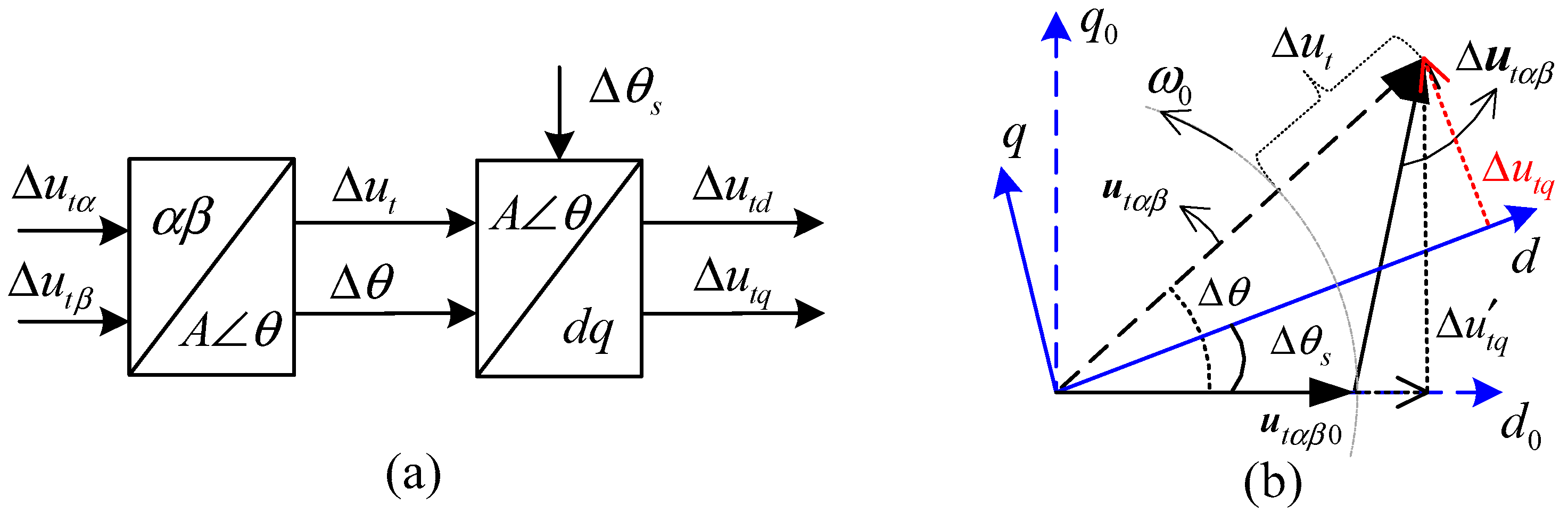
Appendix A. Linearization of the Coordinate Transformation

The specific process of the coordinate transformation linearization is shown in Figure A1a. The linearization of the coordinate transformation in PLL is presented as an example in the following. The coordinate transformation can be written as
u t d q = u t d + j u t q = u t α β e j θ s
where θs is the output phase of SRF-PLL. utαβ can be divided into the steady state operation point part and the small-signal disturbance part in its polar coordinate as
u t α β = u t α β 0 + Δ u t α β = ( U t 0 + Δ u t ) e j ( ω 0 t + θ 0 + Δ θ )
where utaβ0 is the steady-state operation point with the form of periodically time-varying trajectories in the stationary frame. Δutaβ is the small-signal disturbance part. Δut and Δθ are relative small-signal perturbations in the amplitude and phase of utαβ in its polar coordinate system. Unless otherwise stated, the subscript ‘0′ in variables means the steady operation points. Thus, the coordinate transformation in Equation (A1) can be rewritten as follows:
u t d q 0 + Δ u t d q = ( U t 0 + Δ u t ) e j ( ω 0 t + θ 0 + Δ θ ) e j ( ω 0 t + θ s 0 + Δ θ s )
where Δθs is the small-signal output of PLL, and Δutdq is the small-signal disturbance part in the DQ frame. The relation of vectors in (A3) can be intuitively shown in Figure A1b by a vector diagram. The steady state of Equation (A3) is utdq0 = Utej(θ0−θs0). Furthermore, θ0 = θs0 in steady state for a PLL frame is oriented to the utαβ. According to the expansion of Equation (A3), we obtain the following:
Δ u t d q Δ u t + j ( Δ θ Δ θ s ) U t 0
Figure A1. Small-signal variable in SRF-PLL: (a) the diagram description of the linearization of the coordinate transformation in SRF-PLL; and (b) small-signal space vector relations between different frame references.
Energies 11 00374 g0a1
Combining (A2) and (A4), the linearization relation of coordinate transformation in the matrix form is:
[ Δ u t d Δ u t q ] [ 0 Δ θ s U t 0 ] + T s r [ Δ u t α Δ u t β ]

Appendix B. The Expression of Gui+(s), Gui(s), Gue+(s), and Gue(s)

G u i ± ( s ) = ± [ i d 0 / 2 i q 0 / 2 i q 0 / 2 i d 0 / 2 ] T P L L ( s )
G u e ± ( s ) = ± [ e d 0 / 2 e q 0 / 2 e q 0 / 2 e d 0 / 2 ] T P L L ( s )

References

  1. Adams, C.; Carter, C.; Huang, S.H. ERCOT experience with Sub-synchronous Control Interaction and proposed remediation. In Proceedings of the IEEE PES Transmission and Distribution Conference and Exposition, Orlando, FL, USA, 7–10 May 2012; pp. 1–5. [Google Scholar]
  2. Shun-Hsien, H.; Schmall, J.; Conto, J.; Adams, J.; Zhang, Y.; Carter, C. Voltage control challenges on weak grids with high penetration of wind generation: ERCOT experience. In Proceedings of the IEEE PES General Meeting, San Diego, CA, USA, 22–26 July 2012. [Google Scholar]
  3. Zhao, M.; Yuan, X.; Hu, J.; Yan, Y. Voltage Dynamics of Current Control Time-Scale in a VSC-Connected Weak Grid. IEEE Trans. Power Syst. 2015, 31, 2925–2937. [Google Scholar] [CrossRef]
  4. Buchhagen, C.; Rauscher, C.; Menze, A.; Jung, J. BorWin1—First Experiences with harmonic interactions in converter dominated grids. In Proceedings of the International ETG Congress: Die Energiewende—Blueprints for the New Energy Age, Bonn, Germany, 17–18 November 2015; pp. 1–7. [Google Scholar]
  5. Kroutikova, N.; Hernandez-Aramburo, C.; Green, T. State-space model of grid-connected inverters under current control mode. IET Electr. Power Appl. 2007, 1, 329–338. [Google Scholar] [CrossRef]
  6. Wang, Y.; Wang, X.; Blaabjerg, F.; Chen, Z. Harmonic Instability Assessment Using State-Space Modeling and Participation Analysis in Inverter-Fed Power Systems. IEEE Trans. Ind. Electron. 2017, 64, 806–816. [Google Scholar] [CrossRef]
  7. Blasko, V.; Kaura, V. A novel control to actively damp resonance in input LC filter of a three-phase voltage source converter. IEEE Trans. Ind. Appl. 1997, 33, 542–550. [Google Scholar] [CrossRef]
  8. Liserre, M.; Teodorescu, R.; Blaabjerg, F. Stability of photovoltaic and wind turbine grid-connected inverters for a large set of grid impedance values. IEEE Trans. Power Electron. 2006, 21, 263–272. [Google Scholar] [CrossRef]
  9. Brogan, P. The stability of multiple, high power, active front end voltage sourced converters when connected to wind farm collector systems. In Proceedings of the EPE Wind Energy Chapter Seminar, Stafford, UK, 15–16 April 2010. [Google Scholar]
  10. Harnefors, L.; Bongiorno, M.; Lundberg, S. Input-Admittance Calculation and Shaping for Controlled Voltage-Source Converters. IEEE Trans. Ind. Electron. 2007, 54, 3323–3334. [Google Scholar] [CrossRef]
  11. Sun, J. Impedance-Based Stability Criterion for Grid-Connected Inverters. IEEE Trans. Power Electron. 2011, 26, 3075–3078. [Google Scholar] [CrossRef]
  12. Wang, X.; Blaabjerg, F.; Wu, W. Modeling and Analysis of Harmonic Stability in an AC Power-Electronics-Based Power System. IEEE Trans. Power Electron. 2014, 29, 6421–6432. [Google Scholar] [CrossRef]
  13. Wen, B.; Boroyevich, D.; Burgos, R.; Mattavelli, P.; Shen, Z. Analysis of D-Q Small-Signal Impedance of Grid-Tied Inverters. IEEE Trans. Power Electron. 2016, 31, 675–687. [Google Scholar] [CrossRef]
  14. Yuan, H.; Yuan, X.; Hu, J. Modeling of Grid-Connected VSCs for Power System Small-Signal Stability Analysis in DC-Link Voltage Control Timescale. IEEE Trans. Power Syst. 2017, 32, 3981–3991. [Google Scholar] [CrossRef]
  15. Kundur, P. Power System Stability and Control; McGraw-Hill: New York, NY, USA, 1994. [Google Scholar]
  16. He, W.; Yuan, X.; Hu, J. Inertia Provision and Estimation of PLL-Based DFIG Wind Turbines. IEEE Trans. Power Syst. 2017, 32, 510–521. [Google Scholar] [CrossRef]
  17. Sun, J. Small-Signal Methods for AC Distributed Power Systems—A Review. IEEE Trans. Power Electron. 2009, 24, 2545–2554. [Google Scholar]
  18. Dalton, P.M.; Gosbell, V.J. A study of induction motor current control using the complex number representation. In Proceedings of the Conference Record on IEEE Industry Applications Society Annual Meeting, San Diego, CA, USA, 1–5 October 1989; Volume 1, pp. 355–361. [Google Scholar]
  19. Harnefors, L. Modeling of Three-Phase Dynamic Systems Using Complex Transfer Functions and Transfer Matrices. IEEE Trans. Ind. Electron. 2007, 54, 2239–2248. [Google Scholar] [CrossRef]
  20. Sun, J.; Bing, Z.H.; Karimi, K.J. Input Impedance Modeling of Multipulse Rectifiers by Harmonic Linearization. IEEE Trans. Power Electron. 2009, 24, 2812–2820. [Google Scholar]
  21. Cespedes, M.; Sun, J. Impedance Modeling and Analysis of Grid-Connected Voltage-Source Converters. IEEE Trans. Power Electron. 2014, 29, 1254–1261. [Google Scholar] [CrossRef]
  22. Martin, K.W. Complex signal processing is not complex. IEEE Trans. Circuits Syst. I Regul. Pap. 2004, 51, 1823–1836. [Google Scholar] [CrossRef]
  23. Yuan, X.; Merk, W.; Stemmler, H.; Allmeling, J. Stationary-frame generalized integrators for current control of active power filters with zero steady-state error for current harmonics of concern under unbalanced and distorted operating conditions. IEEE Trans. Ind. Appl. 2002, 38, 523–532. [Google Scholar] [CrossRef]
  24. Skogestad, S.; Postlethwaite, I. Multivariable Feedback Control: Analysis and Design; Wiley: New York, NY, USA, 2007. [Google Scholar]
  25. Zhou, J.Z.; Ding, H.; Fan, S.; Zhang, Y.; Gole, A.M. Impact of Short-Circuit Ratio and Phase-Locked-Loop Parameters on the Small-Signal Behavior of a VSC-HVDC Converter. IEEE Trans. Power Deliv. 2014, 29, 2287–2296. [Google Scholar] [CrossRef]
  26. Wen, B.; Dong, D.; Boroyevich, D.; Mattavelli, P.; Burgos, R.; Shen, Z. Impedance-Based Analysis of Grid-Synchronization Stability for Three-Phase Paralleled Converters. IEEE Trans. Power Electron. 2016, 31, 26–38. [Google Scholar] [CrossRef]
Figure 1. Simplified diagram of a voltage source converter (VSC) current control with phase-locked loop (PLL).
Energies 11 00374 g001
Figure 2. Timescale decomposition in VSC control loops.
Energies 11 00374 g002
Figure 3. The process to obtain the current-balancing driven internal voltage motion model, (a) the basic control diagram of the VSC; and (b) the VSC model without input of the terminal voltage.
Energies 11 00374 g003
Figure 4. The process to obtain the current-balancing driven internal voltage motion model of VSC with PLL dynamic, (a) the VSC model with the linearized coordinate transformation; (b) the VSC frequency domain model in a stationary frame; and (c) the internal voltage motion model.
Energies 11 00374 g004
Figure 5. The comparison of the time-domain model and the proposed model: (a) current step responses; and (b) VSC impedance in stationary frame.
Energies 11 00374 g005
Figure 6. The internal voltage and current reference waves in time-domain simulation after a small-signal disturbance.
Energies 11 00374 g006
Figure 7. The frequency curves of the elements in the transfer matrix Gctrl(s) with or without PLL dynamics: (a) the frequency curves of a diagonal element; and (b) the frequency curves of off-diagonal elements.
Energies 11 00374 g007
Figure 8. The frequency curves of elements in matrix Gεu(s)G′ue(s) with the change of PLL bandwidth: (a) the frequency curves of a diagonal element; and (b) the frequency curves of an off-diagonal element.
Energies 11 00374 g008
Figure 9. The system block diagram and frequency characteristic curves of the system transfer function matrix: (a) the block diagram of the studied system, (b) the Nyquist curves of the characteristic loci in Gtotal(s), (c) the real and imaginary part of λtotal1(jω) with changing PLL bandwidth, (d) the real and imaginary part of λtotal2(jω) with changing PLL bandwidth, (e) the real part of −λei1,2(jω), (f) the real part of 1/λctrl1,2(jω).
Energies 11 00374 g009
Figure 10. The experimental results of a grid-connected VSC with changing PLL bandwidth (Time: 50 ms/div, AC voltage: 500 V/div, AC current: 25 A/div).
Energies 11 00374 g010
Table 1. Studied System Parameters.
SymbolQuantityValues (p.u. a)
Lggrid equivalent inductor0.667
Lffilter inductor0.15
Cffilter capacitor0.17
Rddamping resistor1.00
kpcproportionality coefficient of current controller1
kicintegral coefficient of current controller20.0
kpsinitial proportionality coefficient of SFR-PLL0.194
kisinitial integral coefficient of SFR-PLL4.456
a System PU base voltage: 315 V, base power: 10 kVA, and base frequency: 50 Hz.

