Article

An Investigation of Parallel Post-Laminar Flow through Coarse Granular Porous Media with the Wilkins Equation

by
Ashes Banerjee
1,*,
Srinivas Pasupuleti
1,
Mritunjay Kumar Singh
2 and
G.N. Pradeep Kumar
3
1
Departmentof Civil Engineering, Indian Institute of Technology (Indian School of Mines), Dhanbad 826004, Jharkhand, India
2
Department of Applied Mathematics, Indian Institute of Technology (Indian School of Mines), Dhanbad 826004, Jharkhand, India
3
Department of Civil Engineering, SVU College of Engineering, Sri Venkateswara University, Tirupati 517502, Andhra Pradesh, India
*
Author to whom correspondence should be addressed.
Energies 2018, 11(2), 320; https://doi.org/10.3390/en11020320
Submission received: 17 December 2017 / Revised: 23 January 2018 / Accepted: 30 January 2018 / Published: 2 February 2018

Abstract

:
Behaviour of flow resistance with velocity is still undefined for post-laminar flow through coarse granular media. This can cause considerable errors during flow measurements in situations like rock fill dams, water filters, pumping wells, oil and gas exploration, and so on. Keeping the non-deviating nature of Wilkins coefficients with the hydraulic radius of media in mind, the present study further explores their behaviour to independently varying media size and porosity, subjected to parallel post-laminar flow through granular media. Furthermore, an attempt is made to simulate the post-laminar flow conditions with the help of a Computational Fluid Dynamic (CFD) Model in ANSYS FLUENT, since conducting large-scale experiments are often costly and time-consuming. The model output and the experimental results are found to be in good agreement. Percentage deviations between the experimental and numerical results are found to be in the considerable range. Furthermore, the simulation results are statistically validated with the experimental results using the standard ‘Z-test’. The output from the model advocates the importance and applicability of CFD modelling in understanding post-laminar flow through granular media.

1. Introduction

The porous media flow is commonly characterized by the linear relation between the superficial velocity and hydraulic gradient, proposed by Henry Darcy as:
V = k i
where V is the superficial velocity (m/s); i is the hydraulic gradient (head loss per unit length in the direction of flow), and k is the coefficient of permeability (m/s).
However, it is observed that Equation (1) predicts the flow satisfactorily only when the Reynolds number is less than 10 [1,2]. At higher Reynolds numbers, the velocity and hydraulic gradient do not exhibit a linear relationship. Therefore, use of Darcy’s law can cause considerable error in the post-laminar conditions such as the calculation of well productivity [3] and the discharge measurement and design of pumping wells, hydraulic structures such as rock fill dams [4,5], water treatment filters and fissured rocks. Therefore, the characterization and modeling of flow through porous media is pertinent since the issue aptly addresses the abovementioned challenges. Furthermore, the studies and knowledge about the porous media flow can also largely influence efficiency and understanding of the oil and gas exploration which are directly related to the energy sector.
The flow, in the post-laminar regime is mostly described using the Forchheimer equation, as:
i = aV + bV2
where a (s/m) and b (s2/m2) are the Darcy and Non-Darcy coefficients, respectively.
From a thorough review of the literature, one can find enough evidence confirming the complex variation pattern of the Darcy and non-Darcy coefficients with field and media conditions such as porosity, media size, convergent angle, permeability, and so on [6,7,8,9,10,11]. Efforts are made to relate the Darcy and non-Darcy coefficients with the parameters influencing the flow, but they are observed to be empirical therefore of limited use [12,13,14,15,16,17]. The complex variation pattern of the coefficients makes it difficult to predict their values for a given set of media and field conditions. Therefore, modelling of the post-laminar flow, using the Forchheimer type equations often prove to be very difficult.
Since there is no proper equation for representing flow in the non-laminar regime, the search for a single constitutive relation continues even now [18,19].
The Wilkins equation was developed to represent flow in both laminar and non-laminar flow regimes. The equation can be presented as [20]:
V = C 1 μ α r β i γ
where r is characteristic length; α and β are constants; C1 is a coefficient; γ is an exponent having a value between 0.5 and 1.0, depending on the nature of the regime; and μ is the dynamic viscosity of the fluid. For a constant viscosity, Equation (3) can be written as:
V = W r β i γ   with ,   W = C 1 μ α
where W is the modified Wilkins coefficient for a constant viscosity. The coefficients of the Wilkins equation are reported to be relatively non-deviating for media with different hydraulic radius (discussed in Section 2) [21,22,23], unlike the Forchheimer equation [6,20]. The non-deviating nature of Wilkins coefficients encouraged the authors to further investigate the behaviour of these coefficients when subjected to independently varying media sizes and porosities. Further, an effort is made in the present study to simulate the post-laminar flow through porous media with a comprehensive CFD model using ANSYS FLUENT. The model outputs are compared with the experimentally obtained results and further validated statistically using the standard ‘Z-test’. The model outputs and its correlation with the experimental results may advocate the use of such CFD models to analyse and understand the nature and characteristics of post-laminar flow through granular porous media.

2. Experiments and Methodology

A specially conceived parallel flow permeameter with a diameter of 250 mm and a length of 1100 mm is used after packing it with irregularly shaped media having a volume diameter (diameter of a sphere having the same volume as the irregular media) of 29.8 mm, 34.78 mm, and 41.59 mm (Figure 1). To investigate the effect of porosity variation on the flow resistance, velocity behaviour; the same media is repacked three times to achieve separate porosities. The media is packed between two perforated plates and water is allowed to flow at the maximum possible rate for 4 to 5 h to make sure no reorientation of media occurs during the experimentation.
Water is supplied through a header tank (1300 mm × 300 mm × 300 mm) to the permeameter at a constant volumetric flow rate (m3/s). The flow rate is measured as the average of three volumetric flow measurements (m3/s) with an accuracy of ±2.35%. The measured volumetric flow rate m3/s) is divided by the cross sectional area (m2) of the permeameter to obtain the superficial velocity (m/s). For every flow rate, eight separate piezometric head differences are noted from tapings placed vertically over the permeameter at a regular interval of 50 mm. The average hydraulic gradient calculated from the recorded head differences is used for further analysis with an accuracy of ±1.89%. Such an arrangement eliminates any error due to the non-uniformity of packing.
To ensure a post laminar flow condition, experimentations are performed at a higher range of Reynolds number (1736–7194) defined by Kovacs [1,2] as:
Re = V d k ν
where ν = kinematic viscosity (m2/s); dk = characteristic length, defined as d(1 − f)αs/4f; d and αs are the volume diameter (m) and shape factor of the media, respectively.
The ‘hydraulic radius’ (r) [24] (ratio of the void ratio (e) to specific surface (S0)) is used as the characteristic length while calculating the Wilkins coefficients since it includes both parameters (porosity and media size) that influence the flow. The average surface areas and volumes which are prerequisites to calculate the specific surface (surface area per unit volume) are measured as described by Banerjee et al. [23] and presented in Table 1. After measuring the surface area and volume, the volume diameter (diameter of the sphere having the same volume of the media) and the specific surface is calculated.

3. Correction Factors

The experimental setups used in the laboratory are confined in nature, which creates uneven packing in the vicinity of the wall and in the interior of the bed. However, in reality, most of the flows are unconfined in nature. Similarly, during the experimentation, the flow path is assumed to be linear whereas, in reality, it is very tortuous. As a consequence of such constraints, an exact simulation of the field condition in the laboratory is very difficult. In view of the fact that the results obtained in the laboratory cannot be directly applicable to the field, the wall, tortuosity and porosity corrections are applied to the obtained results.

3.1. Wall Correction

The confined boundary wall of the permeameters used in the laboratory causes uneven packing between the media near the walls, which is loosely packed, compared to the media inside. Therefore, the velocity of the flow inside the media and near the wall becomes different. Given that, the media used in the present study are larger in size and the ratio of the permeameter to media diameter is low. Therefore, a wall correction factor developed by Thiruvengadam and Kumar [6] is used to correct the data from any wall effect as follows:
V w = V C w   with   C w = [ ( D + 4.83 × d 2 ) ( D 0.83 × d 2 ) D 2 ] 1
where Vw is the corrected velocity after wall correction, D is the diameter of the permeameter section (mm), and d is the diameter of the porous media used.

3.2. Tortuosity Correction

Generally, the hydraulic gradient is calculated as the ratio of the total head loss to the distance between the tapings, assuming that the flow path is linear in the direction of the pressure loss. However in reality, the fluid flows through the interlinked void spaces within the media. Owing to that, the flow path is mostly non-linear which can cause inaccuracies in the calculation of hydraulic gradient. Therefore, tortuosity corrections are helpful to reduce that error. By definition, tortuosity (τ) is presented as the ratio between the actual lengths of flow between two tapings to the linear distance between them.
The complexity of the porous structure poses a very challenging task while deriving an expression of tortuosity correction factor. Therefore, most tortuosity corrections are empirical in nature obtained from experiments. The Yu and Li [25] model is used here because it theoretically represents a well-defined relationship between tortuosity and porosity. The model presents the tortuosity correction as:
τ = 1 + 1 f ( 1 2 + ( 1 1 f 1 ) 2 + 1 4 1 1 f )
where f is the porosity of the media.

3.3. Porosity Correction

The velocities obtained from the test are calculated by dividing discharge with the cross-section area of the permeameter (superficial velocity), which is different from the velocity inside the media (pore velocity). In order to estimate the actual pore velocity, porosity corrections [26] are introduced as follows:
V v = V f
where Vν is the pore velocity and f is the porosity.
The results are analysed after incorporating all the corrections to their respective parameters as:
V c = V . τ f C w   and   i c = i τ
where Vc and ic are the corrected velocity and hydraulic gradients, respectively.

4. Data Analysis

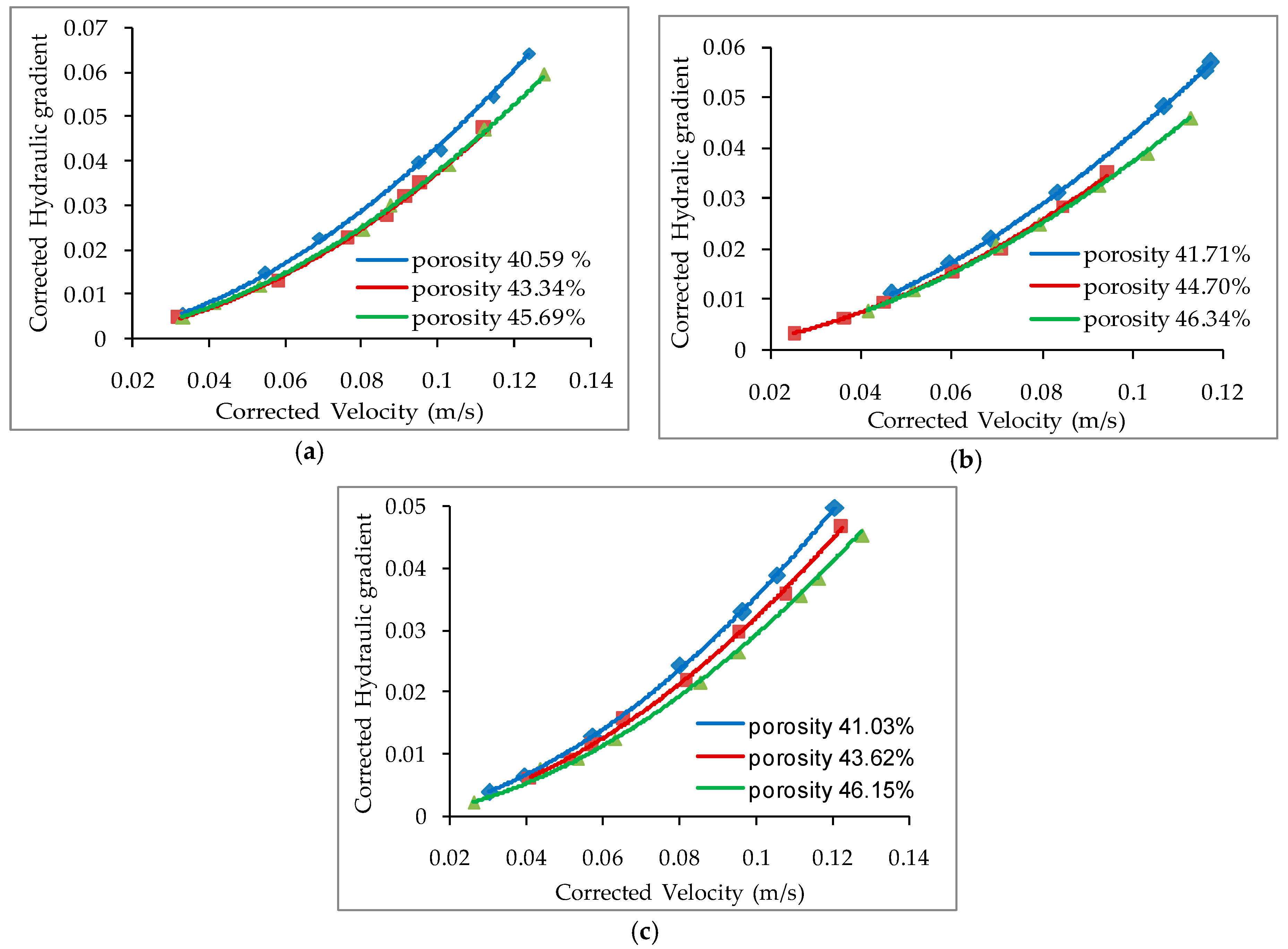
Before the analysis of the data, the following assumptions were made: the flow is single phase and unidirectional, the medium is homogeneous, and the porosity of the medium is uniform. After applying all the corrections in to the experimentally obtained superficial velocities (V) and hydraulic gradients (i), the corrected velocities (Vc) and corrected hydraulic gradients (ic) are plotted in Figure 2 and a relationship in the form of a power law is obtained. This type of equations are also referred as Izbash equation [27] or Missbach equation [20] in the literature:
i c = P V c j
Values of the coefficient P and the exponent j from Equation (10) are calculated from Figure 2. The equation can be modified as follows:
V c = ( i c ( 1 j ) P j )
The Wilkins equation for a constant viscosity can be written as:
V c = W r β i c γ
Thus, judging by the similarity of Equations (11) and (12):
P j = 1 W r β   with   γ = 1 j
1 j log P = ( log W + β log r )
When Equation (14) is plotted in linear form (Figure 3) with −(1/j)log P on the y axis and log r on the x axis, the slope represents the value of the coefficient β and the intercept represents the value of log W. The obtained values of W and β are compared for different media sizes and porosities to understand their effect on the Wilkins coefficients.

5. The Behavior of the Wilkins Coefficients with Independently Varying Media Size and Porosity

Experimentally obtained values for the Wilkins coefficients (W and β) are presented in Table 2. The values of the coefficients are found to be rather constant for all the media experimented with. However, values of γ depend on the flow regime, as mentioned earlier. When compared with the results obtained from earlier reported studies (Table 3), almost similar values of the coefficients are observed. However, it is worth mentioning that the coefficients in the present study vary a little from the ones presented by Banerjee et al. [23]. This may be due to the application of the correction factors. To compare the present experimental results with some of the earlier reported data [28], correction factors are directly applied to the measured velocity and hydraulic gradient instead of modifying the Wilkins equation itself. Since some of the studies have used correction factors where others did not, and the minor differences in the presented results can be attributed to application of correction factors and their different values used to correct the velocity and hydraulic gradient along with the uncertainty and complexity of the porous structure and the human errors during experimentation and calculation. However, one can agree that, for all the reported data, the coefficients of the Wilkins equation present similar values. Furthermore, an attempt is made in the present study to understand the nature of the Wilkins coefficient (W) when the size of the media (volume diameter) and porosity vary independently, after having the coefficients calculated for different hydraulic radius. The values of W are calculated from Equation (12) and plotted for different media sizes whilst keeping the porosity of the packing constant (Figure 4a) and similarly, for different porosities whilst keeping the media size constant (Figure 4b). Figure 4a,b indicate a constant nature of W for media size variation, whereas it shows a slightly increasing trend with porosity when media size is constant.

6. Numerical Modelling

The CFD approach is a very powerful tool for modelling and visualising flows under different conditions. The CFD approach numerically solves three basic equations: the continuity (mass conservation) equation, the motion equation and the energy equation at each point of the computational domain. The ANSYS FLUENT CFD solver, which is based on the Finite Volume method, is used to create and simulate laboratory conditions and to solve the CFD problem.

6.1. Turbulence Modelling

The continuity equation and the momentum conservation (Navier–Stokes) equation for incompressible flow are presented as Equations (15) and (16) respectively:
u i x j = 0
where ui is the velocity component in the xi direction:
ρ u j u i x j = p x j + x j ( μ u i x j ) + ρ g i
where ρ is the density of the fluid, p the pressure, μ is the molecular viscosity and g is the gravitational acceleration.
The turbulent flow is usually simulated after modification of the continuity equation and the momentum conservation (Navier–Stokes) equation for laminar flow with Reynolds decomposition.
The generated quantities known as “Reynolds Stresses” ( ρ u i u j ¯ ) can be defined by the Boussinesq hypothesis using turbulent viscosity (μt) and turbulent kinetic energy (k) [29].
Finally, two additional transport equations need to be incorporated in order to close the equation system representing the turbulent kinetic energy and the turbulence dissipation rate (the k-ε model). The “realizable” k-ε model [30] with a standard wall function is used after a bibliographical study concerning the validation of the CFD model including the realizable k-ε model for a wide range of flows, as well as flows that include the boundary layers and flows over obstacles [30,31].
The two equations for turbulent modelling kinetic energy (k) and turbulence dissipation rate ( ε ) can be written as [29]:
ρ [ x j ( k u j ) ] = x j [ ( μ + μ t σ k ) k x j ] + G k ρ ε
ρ [ x j ( ε u j ) ] = x j [ ( μ + μ t σ ε ) ε x j ] + ρ C 1 S ε ρ C 2 ε 2 k + ν ε
where C 1 = max [ 0.43 ; η η + 5 ] ; C 2 = 1.9; σ k = 1; σ ε = 1.2; η is the time scale ratio defined as =   S k ε with S is the modulus of the mean rate of strain tensor defined by S = 2 S i j S i j ; G k represents the production of the turbulence kinetic energy.
It is worth mentioning that the authors have opted for the standard values of the model constants in the present study since the required model outputs (pressure loss and superficial velocity) are found to be in judicious agreement with the experimental ones. However, the standard values of the model constants may not always provide satisfactory output especially while modelling with no or little turbulence. In such cases, some low Reynolds number closure [32,33,34,35] may be used.

6.2. Model Description

The 3D geometric model with an inlet section, a tank, a parallel flow permeameter, and an outlet section of similar dimensions as the experimental set-up is created using the geometry feature in the ANSYS FLUENT workbench. Owing to the high degree of randomness and the fact that no two porous media shows similar structures at the pore level, it is unnecessary to construct the whole porous media at the fine level as it may not affect the overall physical property of the media. Therefore, the permeameter section is identified as the porous zone with uniform porosity similar to that achieved during experimentation. The porous media is numerically accounted as a momentum sink or a resistance in the momentum equation composed of viscous and inertial terms as given in Equation (19) [29]:
S i = ( j = 1 3 D i j μ v j + j = 1 3 C i j 1 2 ρ | v | v j )
where S i is the source term for ith (x, y or z) momentum equation; | v | is the magnitude of the velocity; D and C are the prescribed matrices. For a homogeneous media:
S i = ( μ α v i + C 2 1 2 ρ | v | v i )
where α is the permeability; C2 is the inertial resistance factor simply specifying D and C as diagonal matrices; and μ and ρ are the dynamic viscosity and the density of the fluid, respectively. The viscous and inertial resistance are measured based on the pressure loss observed from the experimental setup [29,36]. Furthermore, the model is solved by the finite volume method with the velocity pressure coupling done by the SIMPLE algorithm. The governing equations are discretized using the second order upwind differencing scheme. Convergence is attained when the scaled residuals are less than 10−4 times of their initial values.

6.3. Meshing

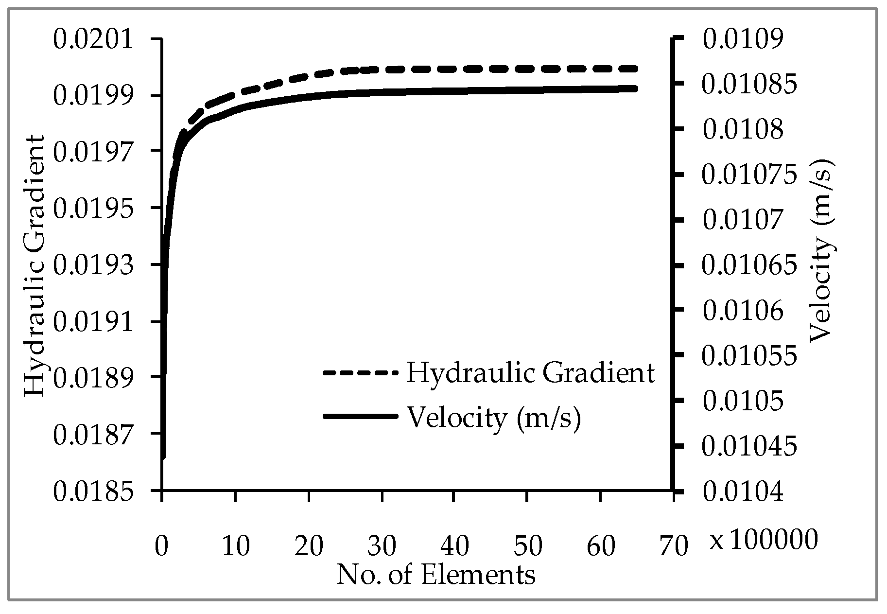
By creating the mesh, a continuous domain describing the flow with partial differential equations is replaced with a finite number of volumes (meshes). The discretization is performed using structured tetrahedral meshes. Nine different grid sizes are selected arbitrarily having element number ranging from 8867 to 6,463,169. Iterative convergence is obtained for each of these grid sizes whilst keeping all other input conditions identical. The output parameters, hydraulic gradient, and velocity are compared for all these meshes which have different numbers of elements. Figure 5 shows that the output parameters become constants as the grid size is refined. Furthermore, a grid sensitivity analysis is performed using the Grid Convergence Index (GCI) method to authenticate the precision of the numerical model [37].
The GCI is the representation of the discretization error between the numerical solutions obtained from the finer grid and the coarser one. For three different selected grids (h1, h2, h3) simulations are carried out to estimate the key variables ( ϕ ); in the present study these variables are Hydraulic gradient, Velocity (m/s) at 0.285 m and Velocity (m/s) at 1.11 m. The apparent order (p) of the method is then calculated using the following equations:
p = 1 ln ( r 21 ) | ln | ε 32 / ε 21 | + q ( p ) |
q ( p ) = ln ( r 21 p [ 1 . sgn ( ε 32 / ε 21 ) ] 32 [ 1 . sgn ( ε 32 / ε 21 ) ] )
where ε 32 = ϕ 3 ϕ 2 , ε 21 = ϕ 2 ϕ 1 , and r 21 = h 2 / h 1 . The equations are solved using fixed-point iteration using the first term as an initial guess [37]. The relative error ( e α 21 , e α 32 ) and the extrapolated relative error ( e e x t 21 , e e x t 32 ) are calculated using Equations (23) and (24):
e a 21 = ϕ 1 ϕ 2 ϕ 1
e e x t 21 = ϕ e x t 21 ϕ 2 ϕ e x t 21   where   ϕ e x t 21 = ( r 21 p ϕ 1 ϕ 2 ) / ( r 21 p 1 )
Finally, the fine Grid Convergence Index (GCI) is calculated using the following equation:
G C I f i n e 21 = 1.25 e a 21 r 21 p 1
Table 4 represents values of these parameters for three selected grids (227,414; 72,709; and 32,301). The output parameters are mentioned as ϕ 1 , ϕ 2 , ϕ 3 or grid sizes h1, h2 and h3 in Table 4. A similar analysis is performed for other selected grid sizes. Numerical uncertainty in the fine grid solution is observed to be 1.09%, 0.56%, and 0.02% respectively for the hydraulic gradient, the velocity at a vertical distance of 0.285 m from the entrance of the permeameter, and the velocity at a vertical distance of 1.11 m from the entrance of the permeameter (Table 4). The GCI values indicate a negligible discretization error and therefore a grid independent solution for the selected grid. Considering the simulation time and precision, a grid system of 1,288,576 elements is adopted for the model.

6.4. Boundary Conditions

The boundary conditions are very important for the numerical solution of the problem. The type and the numerical values of the boundary conditions are carefully chosen. The inlet velocity is calculated by dividing the experimental discharge with the area of the inlet pipe. The turbulent quantities (k and ε) at the inlet are calculated from the Equations (26) and (28) using the turbulent intensity (I); turbulent length scale (l),which depends on the hydraulic diameter (Dh); and the inlet velocity(V) [38]. Equation (26) is used to calculate the turbulent intensity at the core of a fully developed duct [29]:
I = 0.16 ( Re ) ( 1 8 )
The value of k is then calculated using the turbulent intensity from the following equation:
k = 3 2 ( V I ) 2
where Re is the Reynolds number for a pipe flow defined as ρ V d μ .
ε = C μ 3 4 k 3 2 l   with   l = 0.07 D h
The outlet is kept as an outflow boundary, assuming that the flow is completely developed; thereby causing the diffusion flux for all flow variables in the exit direction to be zero [29].

7. Results and Discussion

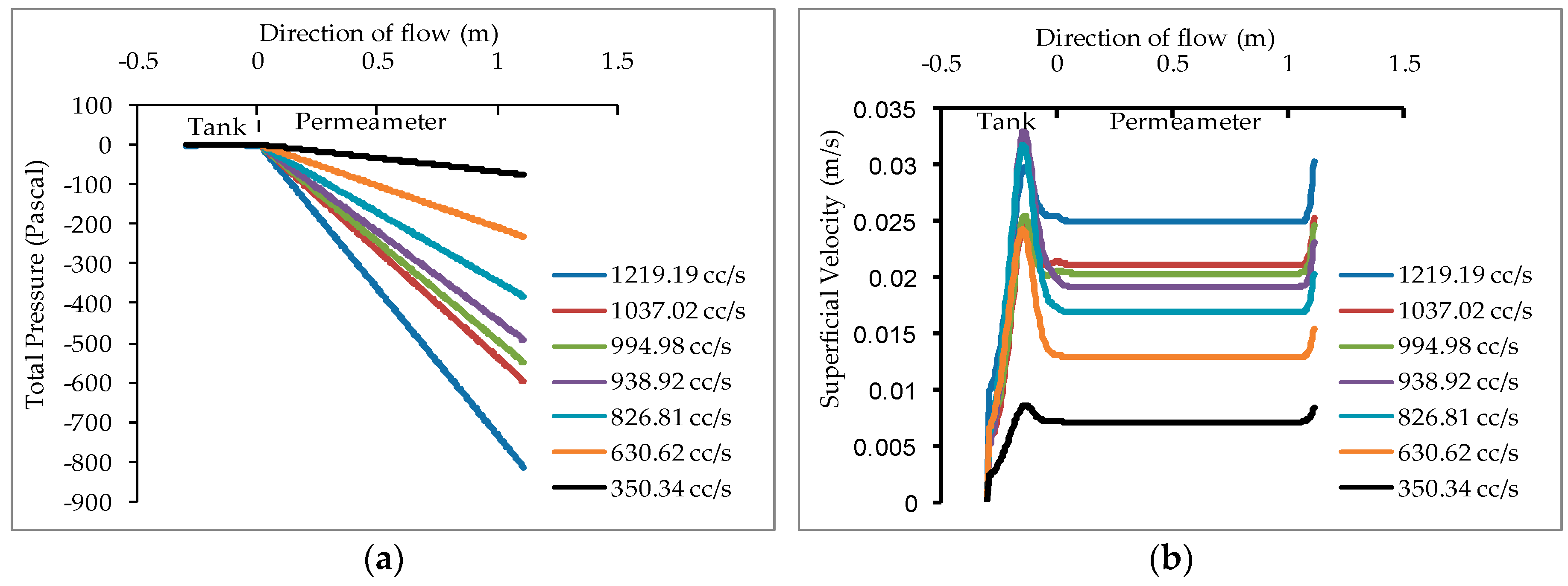
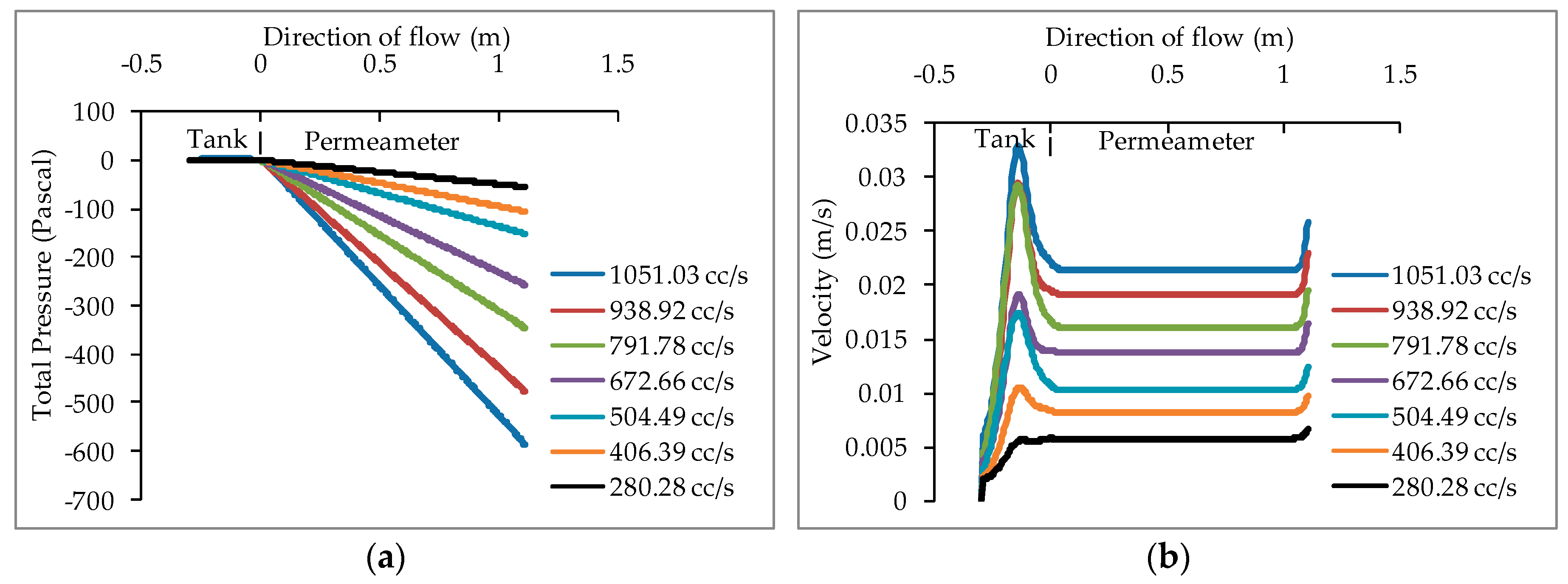
The values of the pressure and velocity along the direction of the flow (length of the permeameter) for the media sizes of 29.8, 34.78 and 41.59 mm are presented in Figure 6a,b, Figure 7a,b and Figure 8a,b, respectively. It can be observed that the total pressure decreases as the flow passes through the length of the permeameter, whereas the velocity plots illustrate a constant superficial velocity throughout the length of permeameter. The pressures and velocities at the tank section (−0.3 m to 0 m) are not used for further analysis since only the permeameter section (0 m to +1.1 m) is identified as a porous zone and subjected to the study. It is worth mentioning that, during the simulation, the operating pressure is set to zero in order to cut down the rounding errors, resulting in negative values in the pressure distribution diagram. However, it does not affect the simulation because of two main reasons; (a) the flow is assumed to be incompressible and (b) the pressure difference is taken into account by the Navier–Stokes equation which drives the flow. The validation of the results and the importance of the model are discussed further in the following sections.

7.1. Comparison between the Experimental and Simulation Data and Statistical Validation of the Simulation

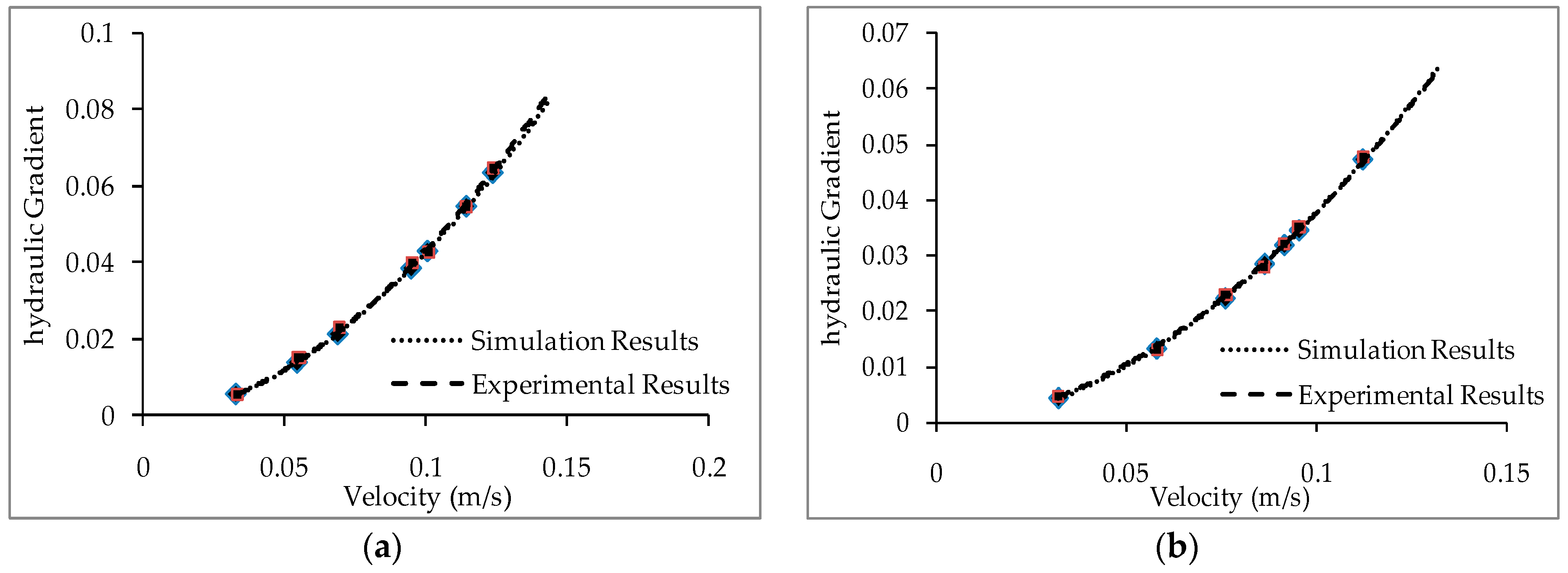
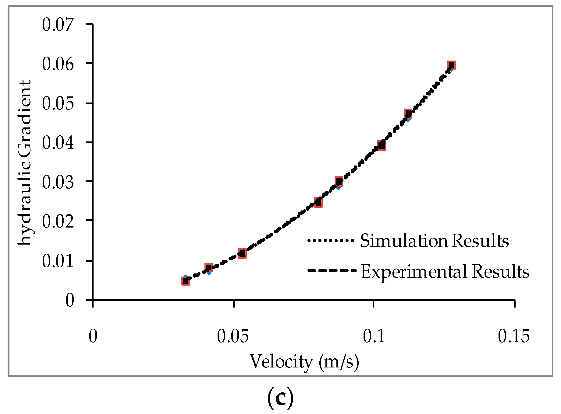
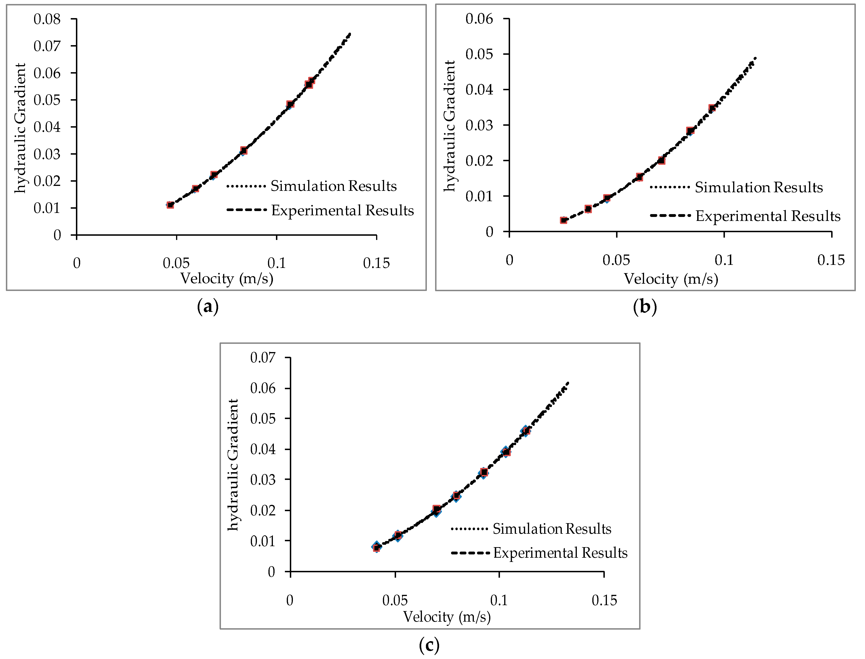
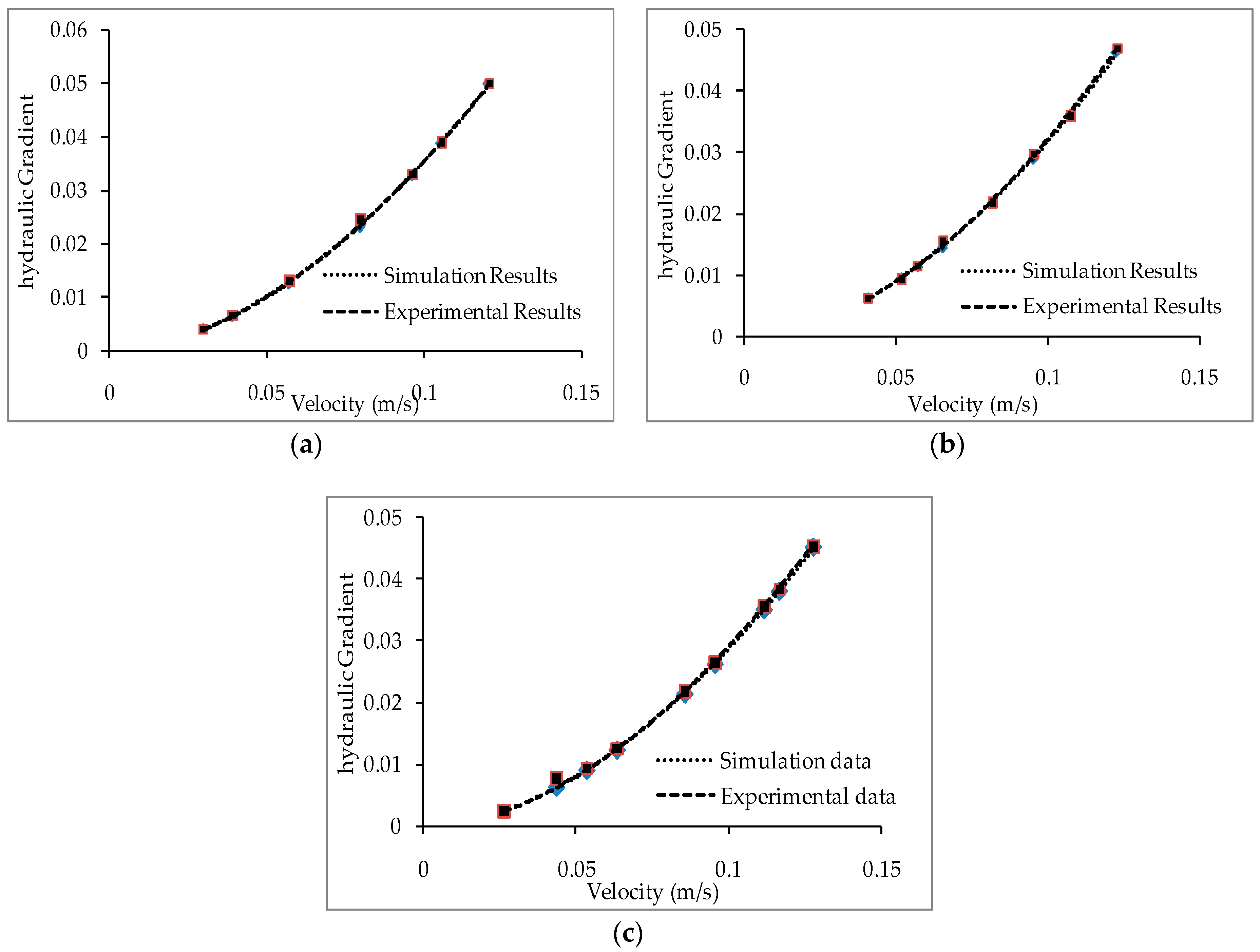
Experimentally and numerically calculated hydraulic gradients are plotted as exponential function (Equation (10)) of the respective velocities in Figure 9a–c, Figure 10a–c and Figure 11a–c. The plots suggest an acceptable correlation between the experimental results and the simulation results for the range of the data tested.
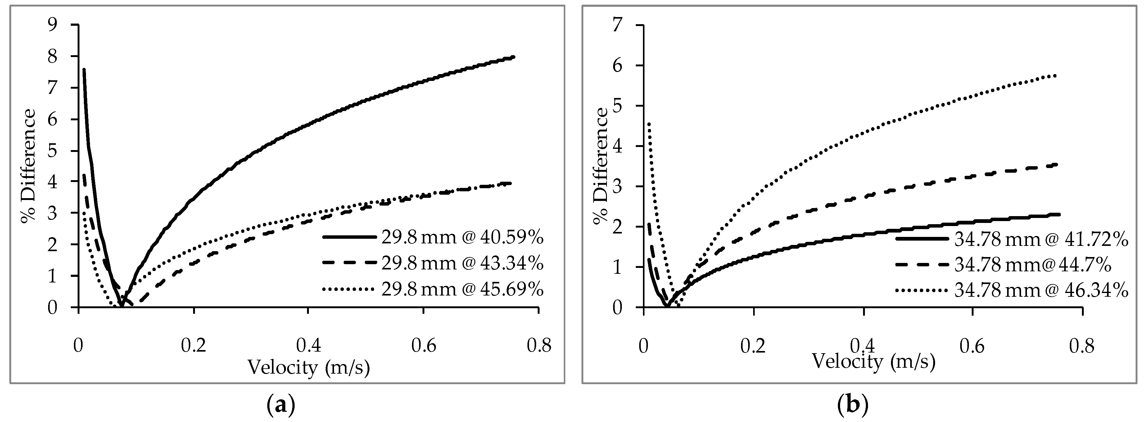
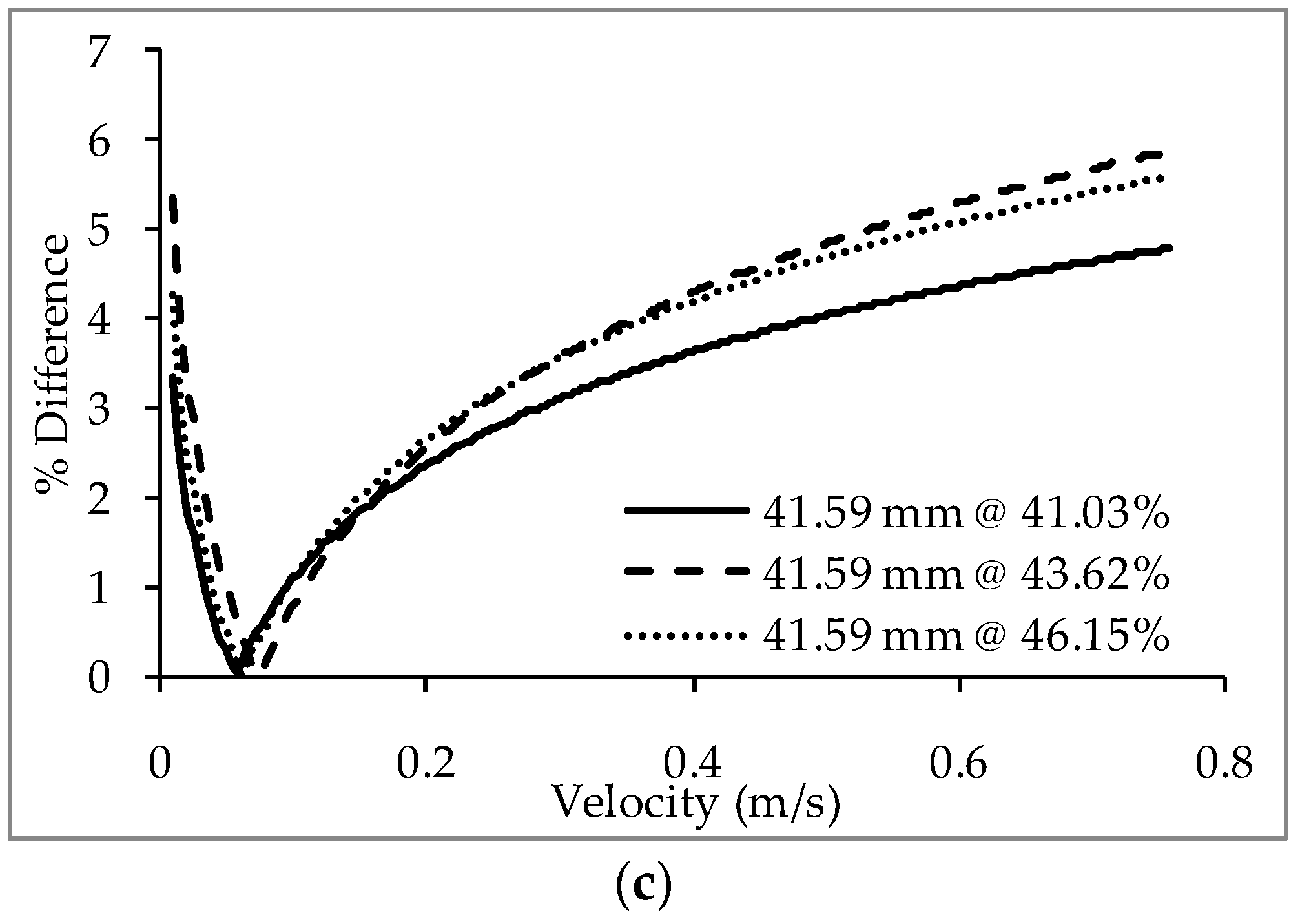
Figure 12a–c represent the percentage deviations between experimental and simulation results applied to the different velocities for all media sizes and porosities. Simulation results are found to be in good agreement with the experimental results for the range of velocities presented. However, the deviation between the simulation and experimental results is not constant. The deviation reduces to a minimum value at a certain velocity and then further increases (Figure 12). This is due to the change in the flow regime with the variation of the velocity. With the change in velocity, the magnitudes of the resistive forces affecting the flow differ, causing a variation in the total resistance thereafter in the velocity-flow resistance relationship. This finally results in a great deviation between the simulation and experimental results. Furthermore, the simulation results have been validated statistically with the experimental results using the standard “Z-test” [39,40], which is explained further in the next section.

7.2. Validation of the Simulated Data Using the Z-Test

In order to test the validity of the simulation result, first the hypothesis is introduced [39,40,41] as follows:
H 0 : μ 1 = μ 2 H 1 : μ 1 μ 2
where μ1 and μ2 are the population mean of the experimental and simulation result. In order to validate the simulated result, the null hypothesis, given by H0, must be accepted.
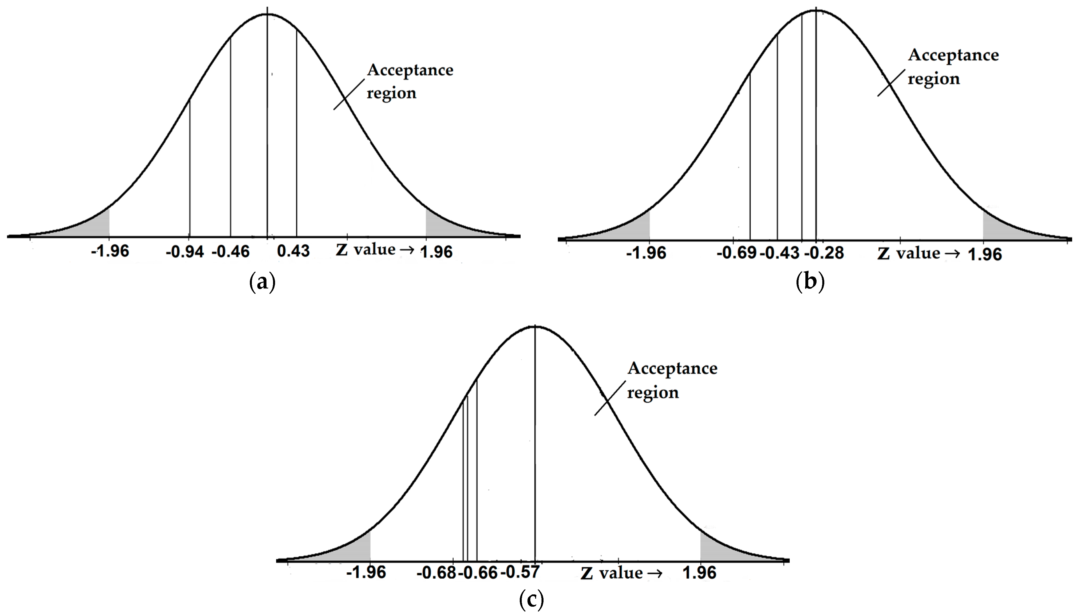
The level of significance (α) is taken to be 5%, which implies that a confidence level of 95% is considered [41]. As the present study deals with two-tailed hypothesis, α = 0.05/2 = 0.025. The corresponding critical value of Z for α = 0.025 is ±1.96 (from the Z table). Therefore, for the hypothesis given as Equation (29) to be accepted, the calculated Z value should be within the interval of [−1.96, 1.96]. The calculated Z values are obtained by employing the Z-test, as given by Equation (30):
Z c a l c u l a t e d = ( x 1 ¯ x 2 ¯ ) ( μ 1 μ 2 ) σ 1 2 N D + σ 2 2 N D   for   N D 30
where x 1 ¯ , x 2 ¯ and μ 1 , μ 2 are the sample and population means for the experimental and simulation results. ND is the total number of data points (sample size) and σ1, σ2 are the standard deviations for the experimental and simulation results.
The results of the Z-test for the three different media sizes are presented in Table 5. The calculated values of Z for all three media sizes are found to be within the acceptable range [−1.96, 1.96] (Figure 13a–c). Therefore, the null hypothesis H0 is accepted, validating the simulation results with the experimental results. Result from the statistical analysis along with the percentage deviation between the simulation and experimental data signify the accuracy of the CFD model used.
This type of CFD model can be very useful to predict the nature of the flow for any hydraulic structure. For a given media size and porosity, this type of simulation can provide a complete velocity and pressure loss profile throughout any given hydraulic structure which can immensely aid the designers and engineers. Furthermore, the obtained velocity and pressure loss data from such models can also be used to analyse the behaviour of different post-laminar flow equations used in porous media flow including the Wilkins equation.

8. Conclusions

A number of non-linear equations were proposed to predict post-laminar flow through porous media at a macroscopic level. However, the complex variation pattern of their respective coefficients limits their applicability in field conditions. The Wilkins equation is studied both theoretically and experimentally with respect to parallel flow. The obtained results are presented as follows:
  • The Wilkins equation can be satisfactorily used to represent post-laminar flow through porous media.
  • The Wilkins coefficients are found to have a non-deviating nature with varying hydraulic radius. The obtained results from the present study are similar to the results reported in the literature.
  • When subjected to variation in media size, the coefficients of the Wilkins equation are constant, given that the porosity is constant. However, variations in the porosity result in small variations of the coefficient W.
  • The flow condition inside the experimental set up is simulated with a CFD model in the ANSYS FLUENT software. Trends similar to the experimental ones are obtained from the simulation results. The percentage deviation between the simulation and experimental results are within the acceptable range.
  • For further validation, the experimental results are statistically compared with the simulation results using the standard Z-test. The values of Z calculated are found to be within the acceptable region for all the experimental results.
Finally, the experimental and simulation results in the present study conclude that the Wilkins equation can represent non-linear flow through porous media with a satisfactory accuracy, compared to Darcy’s equation. The coefficients of the Wilkins equations are found to be constant for variations of porosity and media size, unlike the Forchheimer type equations. Hence, this equation can be regarded as a convenient tool for designing and measuring the discharge for parallel flow through porous media in the non-laminar regimes such as rock fill dams, water filters, aquifers, water, oil and gas wells, and so on.

Acknowledgments

The authors of the present manuscript are thankful to the faculty of IIT (ISM) Dhanbad for extending their facilities during the study. The authors would also like to acknowledge the funding received from IIT(ISM), Dhanbad under the FRS (Faculty Research Scheme) with vide No.: FRS(62)/2013-2014/CE for the fabrication of the permeameter experimental set up utilised in the study.

Author Contributions

Ashes Banerjee, Srinivas Pasupuleti, and G.N. Pradeep Kumar conceived and designed the research. Ashes Banerjee conducted experiments, processed and evaluated the data under the supervision of Srinivas Pasupuleti. Mritunjay Kumar Singh and Srinivas Pasupuleti supervised the data analysis. Ashes Banerjee wrote the manuscript. Srinivas Pasupuleti and Mritunjay Kumar Singh edited the manuscript and also helped in improving the technical content. G.N. Pradeep Kumar outlined the framework of this paper and made key suggestions in improving the method, validation and results.

Conflicts of Interest

The authors declare no conflict of interest. Furthermore, with reference to the received funding from the institute mentioned in the Acknowledgements, there are no conflicts of interest regarding the publication of this manuscript.

References

  1. Kovacs, G. Seepage through saturated and unsaturated layers. Hydrol. Sci. J. 1971, 16, 27–40. [Google Scholar] [CrossRef]
  2. Kovacs, G. Seepage Hydraulics; ESPC: New York, NY, USA, 1981; ISBN 0-444-99755-5. [Google Scholar]
  3. Vincent, M.C.; Pearson, C.M.; Kullman, J. Non-Darcy and multiphase flow in propped fractures: Case studies illustrate the dramatic effect on well productivity. In Proceedings of the SPE Gas Technology Symposium, Calgary, AB, Canada, 30 April–2 May 2002; pp. 71–84. [Google Scholar]
  4. Parkins, A.K.; Trollope, D.H.; Lawson, J.D. Rockfill structures subject to water flow. J. Soil Mech. Found. Div. 1966, 92, 135–151. [Google Scholar]
  5. Curtis, R.P.; Lawson, J.D. Flow over and through rockfill banks. J. Hydraul. Div. 1967, 93, 1–22. [Google Scholar]
  6. Thiruvengadam, M.; Pradip Kumar, G.N. Validity of Forchheimer equation in radial flow through coarse granular media. J. Eng. Mech. 1997, 123, 696–704. [Google Scholar] [CrossRef]
  7. Ergun, S. Fluid flow through packed columns. Chem. Eng. Prog. 1952, 48, 89–94. [Google Scholar]
  8. Nasser, M.S.S. Radial Non-Linear Flow through Porous Media. Master’s Thesis, University of Windsor, Windsor, ON, Canada, 1970. [Google Scholar]
  9. Niranjan, H.S. Non-Darcy Flow through Porous Media. Master’s Thesis, Indian Institute of Technology, Kanpur, India, 1973. [Google Scholar]
  10. Venkataraman, P.; Rao, P.R.M. Darcian, transitional, and turbulent flow through porous media. J. Hydraul. Eng. 1998, 124, 840–846. [Google Scholar] [CrossRef]
  11. Venkataraman, P.; Rao, P.R.M. Validation of Forchheimer’s law for flow through porous media with converging boundaries. J. Hydraul. Eng. 2000, 126, 63–71. [Google Scholar] [CrossRef]
  12. Kumar, G.N.P.; Thiruvengadam, M.; Murali, T. A further study on Forchheimer coefficients as applied in seepage flow. ISH J. Hydraul. Eng. 2004, 10, 1–13. [Google Scholar] [CrossRef]
  13. Reddy, N.B.P.; Rao, P.R.M. Convergence effect on the flow resistance in porous media. Inst. Eng. (I) J. 2004, 85, 36–43. [Google Scholar]
  14. Sadeghian, J.; Kholghi, M.K.; Horfar, A.; Bazargan, J. Comparison of Binomial and Power Equations in Radial Non-Darcy Flows in Coarse Porous Media. J. Water Sci. Res. 2013, 5, 65–75. [Google Scholar]
  15. Bu, S.; Yang, J.; Dong, Q.; Wang, Q. Experimental study of flow transitions in structured packed beds of spheres with electrochemical technique. Exp. Therm. Fluid Sci. 2015, 60, 106–114. [Google Scholar] [CrossRef]
  16. Muljadi, B.P.; Blunt, M.J.; Raeini, A.Q.; Bijeljic, B. The impact of porous media heterogeneity on non-Darcy flow behaviour from pore-scale simulation. Adv. Water Resour. 2016, 95, 329–340. [Google Scholar] [CrossRef]
  17. Li, Z.; Wan, J.; Huang, K.; Chang, W.; He, Y. Effects of particle diameter on flow characteristics in sand columns. Int. J. Heat Mass Transf. 2017, 104, 533–536. [Google Scholar] [CrossRef]
  18. Dukhan, N.; Bağcı, Ö.; Özdemir, M. Experimental flow in various porous media and reconciliation of Forchheimer and Ergun relations. Exp. Therm. Fluid Sci. 2014, 57, 425–433. [Google Scholar] [CrossRef]
  19. Hellström, G.; Lundström, S. Flow through porous media at moderate Reynolds number. In Proceedings of the International Scientific Colloquium Modelling for Material Processing, Riga, Latvia, 8–9 June 2006; pp. 129–134. [Google Scholar]
  20. Kumar, G.N.P.; Venkataraman, P. Non-Darcy converging flow through coarse granular media. J. Inst. Eng. (India) Civ. Eng. Div. 1995, 76, 6–11. [Google Scholar]
  21. Wilkins, J.K. Flow of water through rockfill and its application to the design of dams. N. Zeal. Eng. 1955, 10, 382–387. [Google Scholar]
  22. Garga, V.K.; Hansen, D.; Townsend, R.D. Considerations on the design of flow through rockfill drains. In Proceedings of the 14th Annual British Columbia Mine Reclamation Symposium, Cranbrook, BC, Canada, 14–15 May1990. [Google Scholar]
  23. Banerjee, A.; Pasupuleti, S.; Singh, M.K.; Kumar, G.N.P. A study on the Wilkins and Forchheimer equations used in coarse granular media flow. Acta Geophys. 2017, 1–11. [Google Scholar] [CrossRef]
  24. Scheidegger, A.E. The Physics of Flow through Porous Media; University of Toronto Press: Toronto, ON, Canada; London, UK, 1958. [Google Scholar]
  25. Yu, B.M.; Li, J.H. A geometry model for tortuosity of flow path in porous media. Chin. Phys. Lett. 2004, 21, 1569–1571. [Google Scholar] [CrossRef]
  26. Rose, H.E.; Rizk, A.M.A. Further researches in fluid flow through beds of granular material. Proc. Inst. Mech. Eng. 1949, 160, 493–511. [Google Scholar] [CrossRef]
  27. Sedghi-Asl, M.; Rahimi, H.; Salehi, R. Non-Darcy Flow of Water Through a Packed Column Test. Transp. Porous Media 2014, 101, 215–227. [Google Scholar] [CrossRef]
  28. Kumar, G.N.P. Radial Non-Darcy Flow through Coarse Granular Media. Ph.D. Thesis, Sri Venkateswara University, Tirupati, India, 1994, unpublished. [Google Scholar]
  29. ANSYS Inc. Ansys Fluent 15.0: Users Guide; ANSYS Inc.: Canonsburg, PA, USA, November 2013. [Google Scholar]
  30. Shih, T.H.; Liou, W.W.; Shabbir, A.; Yang, Z.; Zhu, J. A new k–e eddy viscosity model for high Reynolds number turbulent flows. Comput. Fluids 1995, 24, 227–238. [Google Scholar] [CrossRef]
  31. Kim, S.E.; Choudhury, D.; Patel, B. Computations of Complex Turbulent Flows Using the Commercial Code Fluent; ICASE/LaRC Interdisciplinary Series in Science and Engineering; Springer: Dordrecht, The Netherlands, 1997; Volume 7, ISBN 978-94-011-4724-8. [Google Scholar]
  32. Jones, W.P.; Launder, B. The prediction of laminarization with a two-equation model of turbulence. Int. J. Heat Mass Transf. 1972, 15, 301–314. [Google Scholar] [CrossRef]
  33. Chien, K.Y. Predictions of channel and boundary-layer flows with a low-Reynolds-number turbulence model. AIAA J. 1982, 20, 33–38. [Google Scholar] [CrossRef]
  34. Myong, H.K.; Kasagi, N. A new approach to the improvement of k-ε turbulence model for wall-bounded shear flows. JSME Int. J. Ser. 2 Fluids Eng. Heat Transf. Power Combust. Thermophys. Prop. 1990, 33, 63–72. [Google Scholar] [CrossRef]
  35. Crowe, C.T. On models for turbulence modulation in fluid-particle flows. Int. J. Multiph. Flow 2000, 26, 719–727. [Google Scholar] [CrossRef]
  36. Banerjee, A.; Pasupuleti, S.; Kumar, G.N.P.; Dutta, S.C. A Three-Dimensional CFD Simulation for the Nonlinear Parallel Flow Phenomena through Coarse Granular Porous Media. In Lecture Notes in Mechanical Engineering; Springer: Berlin/Heidelberg, Germany, 2018; pp. 469–480. [Google Scholar] [CrossRef]
  37. Celik, I.B.; Ghia, U.; Roache, P.J.; Freitas, C.J.; Coleman, H.; Raad, P.E. Procedure for estimation and reporting of uncertainty due to discretization in CFD applications. J. Fluids Eng. 2008, 130, 0780011–0780014. [Google Scholar] [CrossRef]
  38. Safer, N.; Woloszyn, M.; Roux, J.J. Three-dimensional simulation with a CFD tool of the airflow phenomena in single floor double-skin facade equipped with a venetian blind. Sol. Energy 2005, 79, 193–203. [Google Scholar] [CrossRef]
  39. Camblor, P.M. On correlated z-values distribution in hypothesis testing. Comput. Stat. Data Anal. 2014, 79, 30–43. [Google Scholar] [CrossRef]
  40. Chen, Z.; Nadarajah, S. On the optimally weighted z-test for combining probabilities from independent studies. Comput. Stat. Data Anal. 2014, 70, 387–394. [Google Scholar] [CrossRef]
  41. Mann, P.S.; Lacke, C.J. Introductory Statistics; John Wiley and Sons Inc.: Delhi, India, 2010; ISBN 10:812652734X. [Google Scholar]
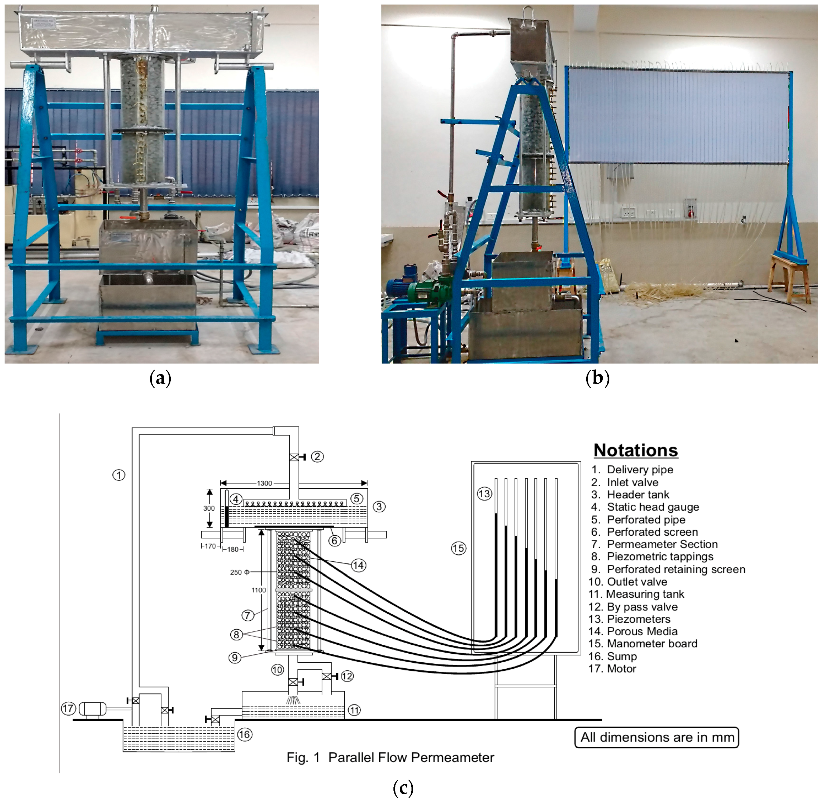
Figure 1. The experimental set-up with the parallel flow permeameter. (a) the front view; (b) the side view; and (c) the schematic diagram.
Energies 11 00320 g001
Figure 2. The variation of corrected hydraulic gradient with a corrected velocity for the media size being (a) 29.8 mm; (b) 34.78 mm; and (c) 41.59 mm.
Energies 11 00320 g002
Figure 3. Equation (14) plotted in a linear form to find out the values of W and β.
Energies 11 00320 g003
Figure 4. Thevariation of W with (a) varying volume diameters of the media with constant porosities and (b) with varying porosity with constant media size.
Energies 11 00320 g004
Figure 5. The variation of the pressure drop with different mesh sizes.
Energies 11 00320 g005
Figure 6. The values of (a) the total pressure and (b) the velocity in the direction of the flow subjected to different discharges for 29.8 mm media packed with 43.34% porosity.
Energies 11 00320 g006
Figure 7. The values of (a) the total pressure and (b) the velocity in the direction of the flow subjected to different discharges for 34.78 mm media packed with 44.70% porosity.
Energies 11 00320 g007
Figure 8. The values of (a) the total pressure and (b) the velocity in the direction of the flow subjected to different discharges for 41.59 mm media packed with 43.62% porosity.
Energies 11 00320 g008
Figure 9. Comparison of simulation and experimental results for 29.8 mm media packed with (a) 40.59%; (b) 43.34%; and (c) 45.69% porosities.
Energies 11 00320 g009aEnergies 11 00320 g009b
Figure 10. Comparison of simulation and experimental results for 34.78 mm media packed with (a) 41.72%; (b) 44.70%; and (c) 46.34% porosities.
Energies 11 00320 g010
Figure 11. Comparison of simulation and experimental results for 41.59 mm media packed with (a) 41.03%; (b) 43.62%; and (c) 46.15% porosities.
Energies 11 00320 g011
Figure 12. The variation of the percentage deviation between the experimental and simulation results with flow velocities for (a) 29.8 mm; (b) 34.78 mm; and (c) 41.59 mm media.
Energies 11 00320 g012aEnergies 11 00320 g012b
Figure 13. The Zcalculated values on the binomial distribution curve for (a) 29.8 mm; (b) 34.78 mm; and (c) 41.59 mm media sizes.
Energies 11 00320 g013
Table 1. Properties of the porous media used.
Passing and Retaining Sieve Sizes (cm)Volume (cm3)Volume Diameter (cm)Avg. Surface Area (cm2)Specific Surface (/cm)
2.50–3.1514.462.9844.682.88
3.15–3.7523.103.4858.442.53
3.75–5.0038.554.1682.112.13
Table 2. The values of the Wilkins coefficient with variation in media size.
Media Size (mm)Porosity (%)W (m-s)βγ
29.8040.596.150.390.54
43.34
45.69
34.7841.725.520.380.56
44.70
46.34
41.5941.035.550.380.55
43.62
46.15
Table 3. The values of the Wilkins coefficients as reported by earlier researchers.
Proposed byMediaVolume Diameter (mm)Porosity (%)W (m/s)βγ
Wilkins (1956) [21]Crushed stone51.0040.005.240.500.54
Garga et al. (1990) [22]Crushed stone24.6047.005.390.500.53
Pradeep Kumar (1994) [27]Crushed stone13.1047.004.940.510.52
20.1045.88
28.9048.73
39.5048.26
Table 4. Sample calculations of numerical uncertainty using the GCI method [37].
ParameterHydraulic GradientVelocity (m/s) at 0.285 mVelocity (m/s) at 1.11 m
h10.0052160.0052160.005216
h20.0069370.0069370.006937
h30.0092260.0092260.009226
r211.331.331.33
r321.331.331.33
ϕ 1 0.019920.010830.01156
ϕ 2 0.019840.010800.01159
ϕ 3 0.019730.010770.01096
P1.327721.3078810.5924
ϕ 21 e x t 0.020100.010880.01156
ϕ 32 e x t 0.020100.010880.01163
e α 21 0.40%0.20%0.27%
e α 32 0.59%0.29%5.45%
e e x t 21 0.86%0.45%0.01%
e e x t 32 1.26%0.65%0.28%
G C I f i n e 21 1.09%0.56%0.02%
Table 5. Values from the Z-test for different media sizes and porosities.
Media Size (mm)Porosity (%)Range of Velocity (m/s) x 1 ¯ x 2 ¯ σ 1 σ 2 N D Z Value
29.8040.590.01–0.7570.6430.5990.5400.359250−0.940
43.340.01–0.7570.5860.6060.4970.5172500.429
45.690.01–0.7570.5540.5350.4640.446250−0.459
34.7841.720.01–0.7570.5650.5540.4630.452250−0.276
44.700.01–0.7570.5270.5100.4350.420250−0.425
46.340.01–0.7570.4960.4710.4070.383250−0.694
41.5941.030.01–0.7570.5110.4890.4220.406250−0.574
43.620.01–0.7570.4640.4400.3910.368250−0.684
46.150.01–0.7570.4390.4180.3690.349250−0.661