Optimization of Wave Energy Converter Arrays by an Improved Differential Evolution Algorithm

Abstract

Since different incident waves will cause the same array to perform differently with respect to the wave energy converter (WEC), the parameters of the incident wave, including the incident angle and the incident wave number, are taken into account for optimizing the wave energy converter array. Then, the differential evolution (DE) algorithm, which has the advantages of simple operation procedures and a strong global search ability, is used to optimize the wave energy converter array. However, the traditional differential evolution algorithm cannot satisfy the convergence precision and speed simultaneously. In order to make the optimization results more accurate, the concept of an adaptive mutation operator is presented to improve the performance of differential evolution algorithm. It gives the improved algorithm a faster convergence and a higher precision ability. The three-float, five-float, and eight-float arrays were optimized, respectively. It can be concluded that the larger the size of the array is, the greater the interaction between the floats is. Hence, a higher efficiency of wave energy extraction for wave energy converter arrays is achieved by the layout optimization of the array of wave energy converters. The results also show that the optimal layout of the array system is inhomogeneously distributed and that the improved DE algorithm used on array optimization is superior to the traditional DE algorithm.

1. Introduction

Consumption of fossil energy, such as oil, coal, and natural gas, has grown rapidly with the industrialization process. It is highly necessary to capture natural energy resources and convert them into electric energy or heat, going beyond non-renewable energy. Currently, the earth’s surface area is 510 million km², the ocean area of which is 361 million km², accounting for 71% of the total area. It is estimated that the marine energy accounts for more than 70% of the world’s total energy [1]. China is a marine country whose sea area is vast and whose marine resources are abundant. Thus, the comprehensive utilization of marine energy has been proposed in China.

There is a large amount of renewable energy in the ocean, including wave energy, thermal energy, wind energy, salinity energy, tidal current energy, and tidal energy [2]. Wave energy has gained considerable attention owing to its greater energy density compared to others. It is estimated that the wave energy reserve in the world is about 2.5 billion kW [3]. As early as a century ago, people began to explore how wave energy can be used to generate electricity [4,5]. There are various kinds of wave energy converters, such as point absorbers, attenuators, and terminators [6].

However, a single WEC has a low power efficiency, unstable power generation, and only small-scale generated electricity because it generally cannot absorb the ocean wave energy in different positions and directions at the same time [7,8]. Therefore, multiple WECs are arranged as an array to generate more power so as to improve the efficiency of wave power generation. Although the research on the WEC array is still in its infancy, many related devices have been developed and put into practice.

Research on wave energy converter arrays began in the late 1970s. The method of approximating WEC to a point absorber was used by Budal [9] to simplify calculations. The scattered wave field could be neglected due to the assumed small devices. Multiple body diffraction was later applied to axisymmetric wave energy converter arrays in [10]. Yilmaz and Incecik [11,12] merged the solution of a single WEC [13] with the interaction process of an array, which was studied by Kagemoto and Yue [14]. In addition, the influences of radiation were taken into consideration when all devices moved together. Child and Venugopal [15] applied a parabolic cross algorithm and a genetic algorithm to optimize arrays of wave energy converters. The differential evolution (DE) algorithm was introduced to design the geometry size of a WEC by Blanco [16] and others according to the type, position, hydrodynamics, parameters, and control strategy of devices. The array configuration of two and four devices was determined by simulating the array in the time domain with a coupled hydrodynamic-electromagnetic model [17]. Ruiz investigated the algorithms of seeking an optimal layout between WECs in different orientations and positions [18]. Ferri [19] applied derivative-free global optimization algorithms to explore the optimal energy absorbed by WEC arrays. MILDwave was used to model WEC arrays by Verbrugghe et al. [20]. A glowworm swarm optimization algorithm, a genetic algorithm, and a covariance matrix adaptation evolution strategy were compared in terms of performance with respect to WEC arrays and computational cost, and the covariance matrix adaptation evolution strategy had less computational complexity and slightly lower accuracy [21]. Thomas [22] and others presented a robust and reliable control strategy, called the model-free collaborative learning method, for WEC arrays in irregular wave conditions. Further, a novel approach that combines the MILDwave wave-propagation model with NEMOH BEM model was adopted to explore how the distance of the WEC array affects the generating efficiency [23].

In addition, at the University of Edinburgh, UK, a five-float array was analyzed, and the results showed that the array had higher energy efficiency than did a single-float array in an optimized state. Dr. David Forehand from this university created software called OceanEd [24], in which the WECs of an array can be designed with any shape, layout, and degrees of freedom, to work out and test linear hydrodynamic time-domain models of rigid-body WEC arrays [25]. Ghent from the University of Belgium conducted an experiment of a 5 × 5-float array in a wave tank in a laboratory, focusing on the interaction between the floats. The FO3 wave energy converter was developed at Norway’s Oslo University, in which a 1:20 scale simulation was performed in a wave tank and a 1:3 scale experiment was carried out in real sea conditions. Additionally, a multi-float array wave energy converter test system called “Trident” was built by the Trident Energy Company (Blyth, UK ). The advantages of this system are the small distance between the floats and the linear machines used to generate electricity. In China, WEC arrays have also been studied in many colleges. For example, an WEC array named “Motor Wave” was developed in Hong Kong University. The “Haiyuan No. 1” wave energy converter platform, which has three oscillation floats, was carried out at Zhejiang Ocean University. A four-float wave energy converter was developed at China Ocean University as well [26].

An array of oscillating buoy WECs, which are point-absorber WECs, was studied here. The influences of incident angle β and incident wave number k₀ on the WEC array were examined. These two incident wave parameters will influence the efficiency and output of WEC arrays. It was found that, when the incident angle is set to zero and the wave number satisfies 2ak₀ = 0.8 (a is the radius of float), a larger interaction coefficient can be obtained. This can be used to research the layout optimization of WEC arrays. Further, the DE algorithm was used to optimize the WEC array. In addition, the concept of an adaptive mutation operator is introduced to modify the DE algorithm, which not only meets the requirements in calculation convergence speed but also makes the optimization result more accurate. The adaptive mutation operator shows that a larger mutation operator F used at an early stage prevents population diversity from local convergence and that a smaller F used later ensures accuracy with minimum error. The value of F is maintained in the best range for optimization results. The positions of each WEC in the array are determined by the improved DE algorithm, under more suitable incident wave parameters, so that greater wave energy is extracted from the ocean. The results show that the optimal layout is inhomogeneously distributed and that there are improved results after modification.

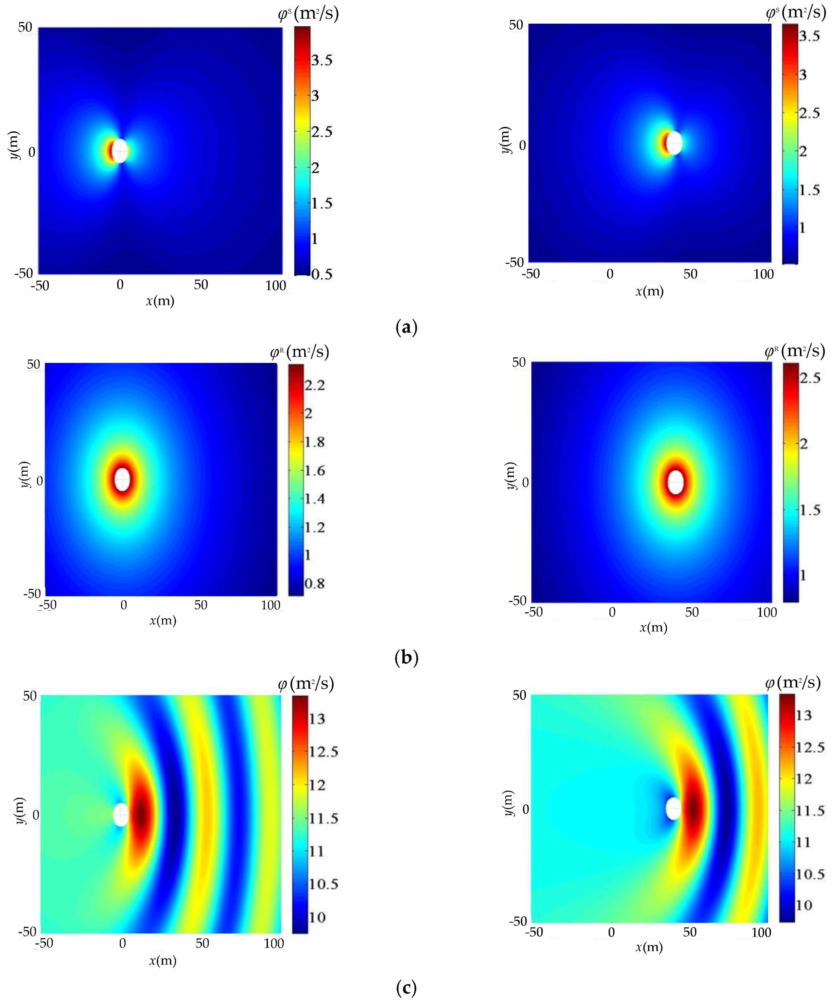
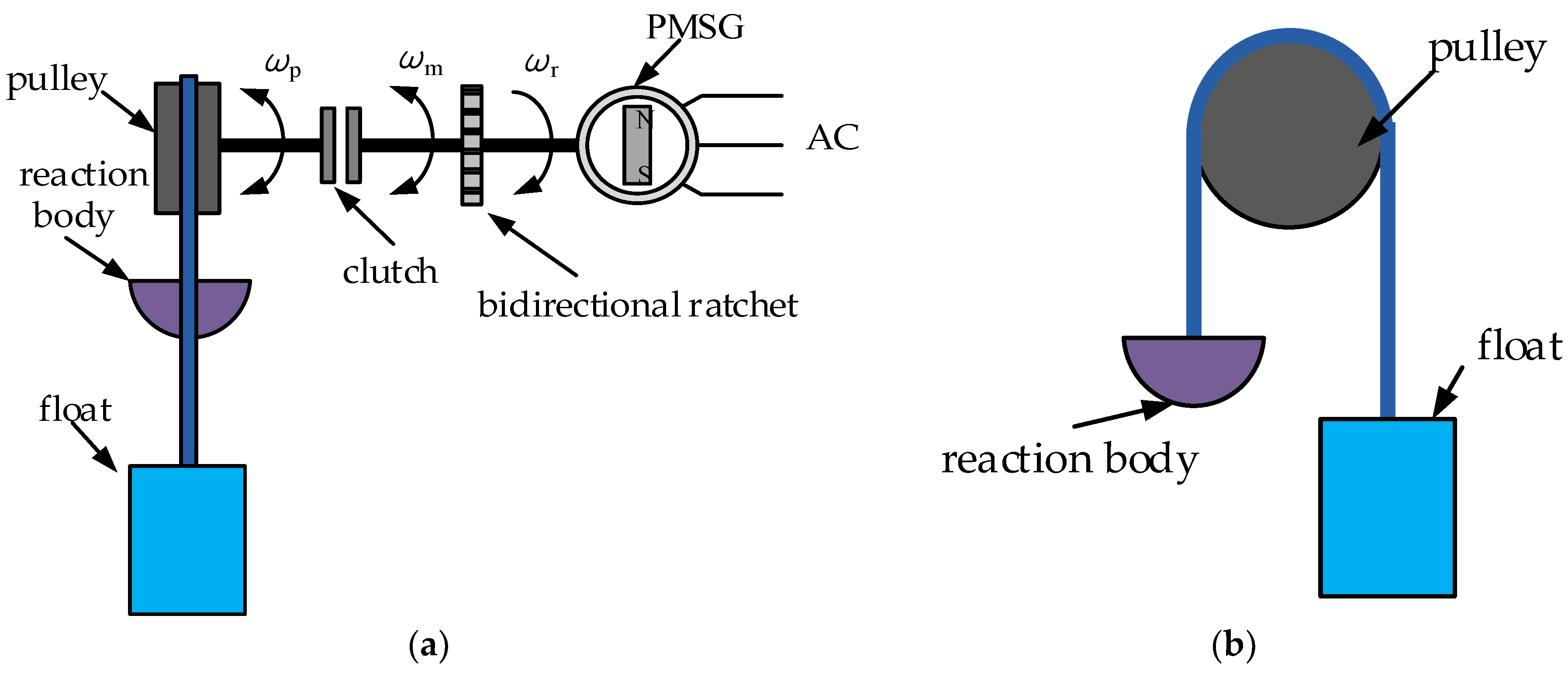
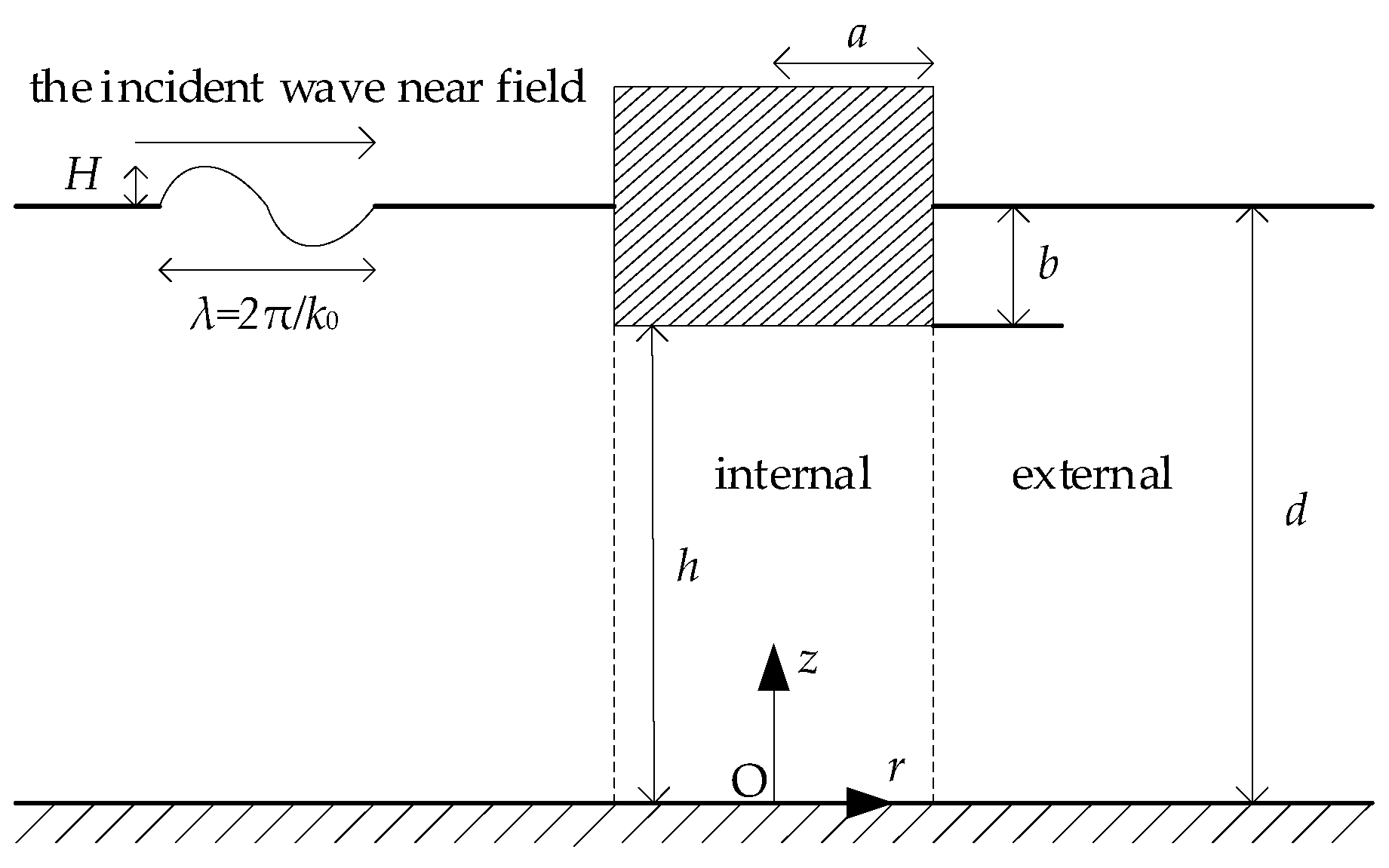
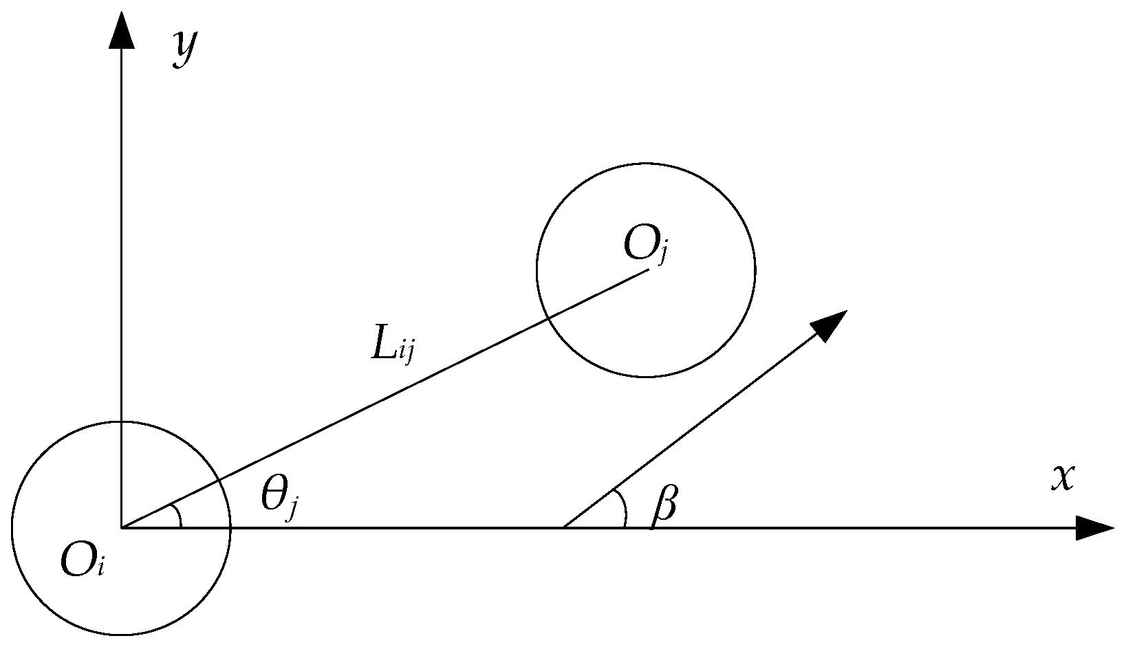
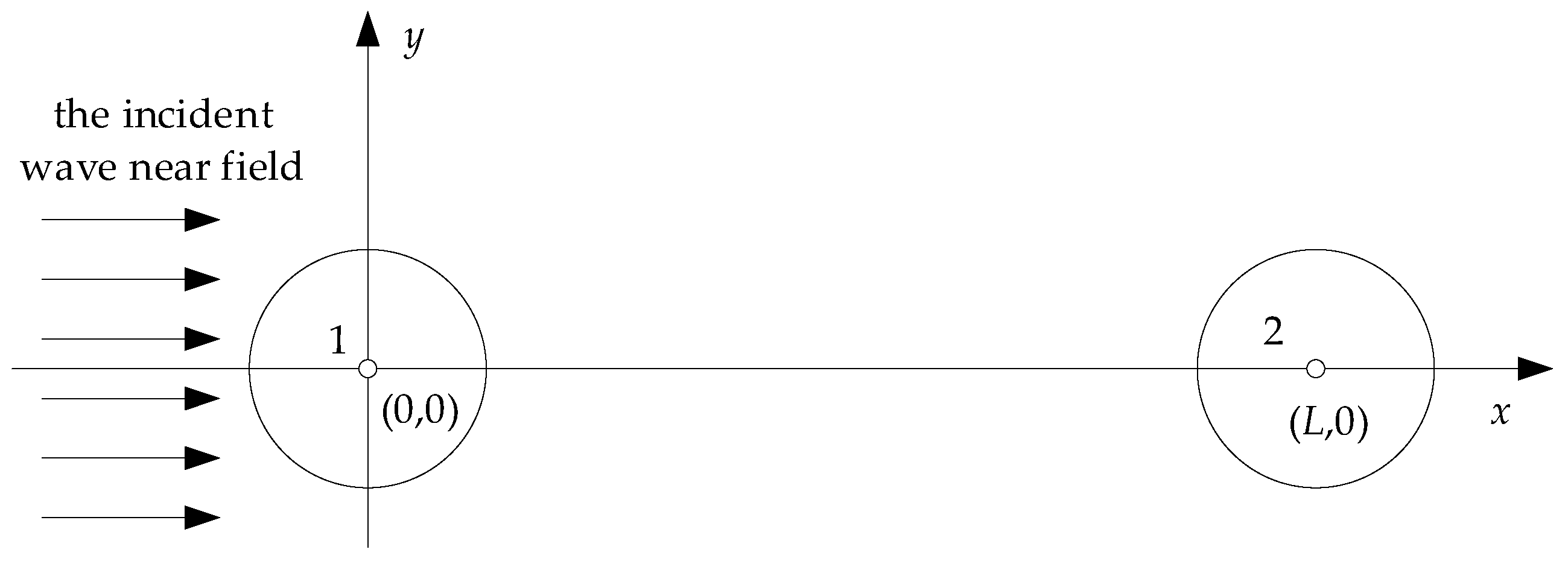
2. The Hydrodynamic Model of an Array System

In this paper, an improved oscillating buoy WEC system is adopted as shown in Figure 1. This system has a strong adaptability in nearshore and offshore regions. The float in the figure is connected with the reaction body through a pulley. The float can move up and down so that the wave energy can be converted to drive the permanent magnet synchronous generator (PMSG) continuously. The PMSG will then rotate in one direction under the automation control of the clutch and the bidirectional ratchet. The reaction body can maintain the cable tension and control the natural frequency of the WEC [27].

In this paper, it is supposed that the fluid is non-viscous and the fluid density ρ is invariable. The depth of the water is a finite value d, and the equation of wave free plane is z [28]. The corresponding float model is cylindrical, and the state of it in seawater can be simplified as shown in Figure 2.

In Figure 2, in the polar coordinate system, the submerging depth of the float is b, and the distance between the bottom of the float and the seafloor is h (h = d − b). The radius of the float is a. The size of the array is N (i.e., there are N floaters), and each float is numbered by j, j ∈ 1, 2, 3, …, N, where the radius of float j is a_j, and the quality is M_j. When 0 ≪ r_j ≪ a_j, it represents the internal zone of float j. When r_j ≫ a_j, it represents the external zone of float j. The elastic effect of the cable can be equivalent to a spring with a coefficient of elasticity δ_j and a damper with a damping coefficient of γ_j [29]. Further, it is assumed that the center coordinate O_i of the float i is (0, 0), the center coordinate O_j of the float j is (x_j, y_j), the distance between O_i and O_j is L_ij, the angle between the positive direction of the z-axis and the connecting line of float j and float i is θ_ij, and β is the angle between the incident direction and the abscissa. The amplitude of the incident wave near field is H, the wave number is k₀, the wave length is λ = 2π/k₀, and the acceleration of gravity is g. The example of the two-float array in the Cartesian coordinate system is shown in Figure 3.

The analysis is under the theory of linearized potential flow, which has been validated in [30]. The wave energy absorbed by the float can be calculated by the velocity potential φ, which can be decomposed into three components as [15,28,31]

$$\phi ={\phi }^{\mathrm{I}}+{\phi }^{\mathrm{S}}+{\phi }^{\mathrm{R}}={\phi }^{\mathrm{A}}+{\phi }^{\mathrm{D}}$$

(1)

where φ^I represents the velocity potential of the incident wave, φ^S represents the scattered waves, φ^R represents the radiated waves, φ^D = φ^I + φ^S represents the velocity potential of the diffraction wave, and φ^A represents the velocity potential of the incident wave near field. The φ^A of the j-th float [32] is

$${\phi }_j^{\mathrm{A}}=\frac{gH}{\omega }{\mathsf{\alpha }}_j^T{\mathit{\Psi }}_j^I$$

(2)

where the angular frequency ω satisfies that ω² = −k_m × g × tan(k_m × d), and k_m is the wave number of the evanescent wave. The superscript T in α_j indicates the transpose, and the Ψ_j^I and α_j are represented as follows [14]:

$${({\mathit{\Psi }}_j^{\mathrm{I}})}_m^n=\{\begin{array}{cc}\frac{\cosh k_{0}z{J}_n(k_0{r}_j)}{\cosh k_{0}d{J}_n(k_0{a}_j)}{\mathrm{e}}^{\mathrm{i}n{\theta }_j},& m=0\\ \cos k_{m}z\frac{I_n(k_m{r}_j)}{I_n(k_m{a}_j)}{\mathrm{e}}^{\mathrm{i}n{\theta }_j},& m\ge 1\end{array}$$

(3)

$${({\mathsf{\alpha }}_j)}_m^n=\{\begin{array}{ll}{I}_j{J}_n(k_0{a}_j){\mathrm{e}}^{\mathrm{i}n(\pi /2-\beta )},& m=0\\ 0,& m\ge 1\end{array}$$

(4)

where J_n is the n-order primal Bessel function, I_n is the n-order modified primal Bessel function, and I_j is the phase conversion factor of float j from the Cartesian coordinate system to the polar coordinate system. m (0 ≤ m ≤ +∞) is the discretization value of the z-axis in the Cartesian coordinate system. n (−∞ ≤ n ≤ +∞) is the discretization value of the θ axis in the polar coordinate system.

In the external zone of the j-th float, the scattered wave velocity potential φ^S [31,33] is expressed as

$${\phi }_j^{\mathrm{S}}=\frac{gH}{\omega }{\mathit{A}}_j^{\mathrm{T}}{\mathit{\Psi }}_j^{\mathrm{S}}=\frac{gH}{{\omega }_p}P{\mathit{A}}_j^{\mathrm{T}}{\mathit{T}}_{ji}{\mathit{\Psi }}_i^{\mathrm{I}}$$

(5)

where A_j^T is a coefficient matrix of float j, and the matrix for coordinate transform T_ji from Ψ_j^S to Ψ_i^I is represented as

$${(T_{ji})}_{mm}^{nl}=\{\begin{array}{ll}\frac{J_l(k_0{a}_i)}{H_n(k_0{a}_j)}{H}_{n-l}(k_0{L}_{ji})e^{\mathrm{i}{\theta }_j(n-l)},& m=0\\ \frac{I_l(k_m{a}_i)}{K_n(k_m{a}_j)}{K}_{n-l}(k_m{L}_{ji})e^{\mathrm{i}{\theta }_j(n-l)}{(-1)}^l,& m\ge 1\end{array}$$

(6)

where H_n is the n-order primal Hankel function, and K_n is the n-order modified second Bessel function.

For the velocity potential of the incident wave near field, the value of the external zone of the float is different from that of the interior case. The internal scattering wave and the incident wave near field of the float are difficult to distinguish. Therefore, φ^D is referred to as the diffraction wave field in the interior region of the float. In the interior region of the j-th float, φ^D is expressed as

$${\phi }_j^{\mathrm{D}}=\frac{gH}{\omega }{\tilde{\mathit{A}}}_j^{\mathrm{T}}{\tilde{\mathit{\Psi }}}_j^{\mathrm{D}}$$

(7)

where ${\tilde{\mathit{\Psi }}}_j^{\mathrm{D}}$ is calculated as

$${({\tilde{\mathit{\Psi }}}_j^{\mathrm{D}})}_m^n=\{\begin{array}{ll}{(\frac{r_j}{a_j})}^{\left|n\right|}{\mathrm{e}}^{\mathrm{i}n{\theta }_j},& m=0\\ \cos (m\pi z/h_j)\frac{I_n(m\pi r_j/h_j)}{I_n(m\pi a_j/h_j)}{\mathrm{e}}^{\mathrm{i}n{\theta }_j},& m\ge 1\end{array}$$

(8)

where z = h_j.

Further, in the external region of the j-th float, the radiated wave field φ^R can be represented as

$${\phi }_j^{\mathrm{R}}=\frac{gH}{\omega }{\widehat{X}}_j{R}_j(r_j,z)=\frac{gH}{\omega }\widehat{X}{R}_j^{\mathrm{T}}{\mathit{\Psi }}_j^{\mathrm{S}}$$

(9)

where R_j(r_j, z) is the radiation characteristic coefficient of the exterior region for float j, and ${\widehat{X}}_j$ is the non-dimensional motion amplitude of float j, which is the movement amplitude of the float.

In the interior region of the j-th float, the radiated wave field φ^R is represented as

$${\phi }_j^{\mathrm{R}}=\frac{gH}{\omega }{\widehat{X}}_j{\tilde{R}}_j(r_j,z)=\frac{gH}{\omega }{\widehat{X}}_j\left[{\tilde{R}}_j^{\mathrm{P}}+{\tilde{\mathit{R}}}_j^{\mathrm{T}}{\tilde{\mathit{\Psi }}}_j^{\mathrm{D}}\right]$$

(10)

where ${\tilde{R}}_i(r_i,z)$ is the radiation characteristic coefficient of the inner region for the j-th float. The ${\tilde{R}}_{}^{\mathrm{P}}$ satisfies ${\tilde{R}}^{\mathrm{p}}=-\mathrm{i}{\omega }^2\left(z^2-r^2/2\right)/(2gh)$, where $0\le r\le a$.

The expression of the total velocity potential of incident wave is represented as

$${\phi }_j^{\mathrm{I}}=\frac{gH}{\omega }\left[{\mathit{\alpha }}_j^{\mathrm{T}}+{\displaystyle \sum _{\begin{array}{l}i=1\\ i\ne j\end{array}}^N{({\mathit{A}}_i+{\widehat{X}}_i{\mathit{R}}_i)}^{\mathrm{T}}{\mathit{T}}_{ij}}\right]{\mathit{\Psi }}_j^{\mathrm{I}}.$$

(11)

A transformation matrix B_j is adopted to show a relationship between the coefficient Ψ_j^I in Equation (11) and the coefficient Ψ_j^S in Equation (9) as

$${\mathit{A}}_j={\mathit{B}}_j\left[{\mathit{\alpha }}_j+{\displaystyle \sum _{\begin{array}{l}i=1\\ i\ne j\end{array}}^N{\mathit{T}}_{ij}^{\mathrm{T}}({\mathit{A}}_i+{\widehat{X}}_i{\mathit{R}}_i)}\right].$$

(12)

Similarly, a transformation matrix ${\tilde{\mathit{B}}}_j$ could be introduced to represent the relationship between the coefficient Ψ_j^I in Equation (11) and the coefficient ${\tilde{\mathit{\Psi }}}_j^{\mathrm{D}}$ in Equation (7) within the float as

$${\tilde{\mathit{A}}}_j={\tilde{\mathit{B}}}_j\left[{\mathit{\alpha }}_j+{\displaystyle \sum _{\begin{array}{l}i=1\\ i\ne j\end{array}}^N{\mathit{T}}_{ij}^{\mathrm{T}}({\mathit{A}}_i+{\widehat{X}}_i{\mathit{R}}_i)}\right].$$

(13)

Combining Equations (7), (10), and (13), the velocity potential inside the float j can be calculated, so it is easy to calculate the fluctuating force of the wave.

$${\phi }_j=\frac{gH}{\omega }\left\{\left[{\mathit{\alpha }}_j^{\mathrm{T}}+{\displaystyle \sum _{\begin{array}{l}i=1\\ i\ne j\end{array}}^N{({\mathit{A}}_i+{\widehat{X}}_i{\mathit{R}}_i)}^{\mathrm{T}}{\mathit{T}}_{ij}}\right]{\tilde{\mathit{B}}}_j^{\mathrm{T}}{\tilde{\mathit{\Psi }}}_j^{\mathrm{D}}+{\widehat{X}}_j({\tilde{R}}_j^{\mathrm{P}}+{\tilde{\mathit{R}}}_j^{\mathrm{T}}{\tilde{\mathit{\Psi }}}_j^{\mathrm{D}})\right\}.$$

(14)

The Bernoulli equation is applied to integrate the bottom of the float S_j. Then, in the positive direction of the z-axis, the hydrodynamic forces of float ($F_j^{\mathrm{H}}$) can be calculated as

$$F_j^{\mathrm{H}}=i\omega \rho {\displaystyle {\iint }_{S_j}{\phi }_j}(r_j,{\theta }_j,h_j)\mathrm{d}\mathrm{S}.$$

(15)

The elastic force $F_j^{\mathrm{B}}$ represents the buoyancy and gravity of a float in water, as follows

$$F_j^{\mathrm{B}}=-\rho \pi a_j^2{X}_{j}g$$

(16)

where X_j is the movement amplitude of float in the wave, which satisfies $X_j=H{\widehat{X}}_j$. Furthermore, the float is pulled by the rope, and the elastic effect of the cable can be equivalent to a spring with an elastic coefficient of δ_j and a damper with a damping factor of γ_j. Therefore, the tension of a cable can be expressed as follows:

$$F_j^{\mathrm{G}}=-{\delta }_j{X}_j-{\gamma }_j{X}_j^{\prime }$$

(17)

where $X_j^{\prime }$ is the speed of the float in the wave, which satisfies $X_j^{\prime }=-i\omega H{\widehat{X}}_j$.

By combining Equations (15)–(17), the following equation can be obtained:

$$M_j{X^{″}}_j=F_j^{\mathrm{H}}+F_j^{\mathrm{B}}+F_j^{\mathrm{G}}$$

(18)

where $X_j^{″}$ is the acceleration of a float in the wave, which satisfies $X_j^{″}=-i{\omega }^{2}H{\widehat{X}}_j$, M_j is the quality of the float, which satisfies $M_j=\rho \pi a_j^2(d-h_j)$.

A_i and ${\widehat{X}}_j^{}$ are then given based on the above equations. Therefore, the wave energy extracted from each float can be calculated as [34]

$$P_j=\frac{1}{2}{\gamma }_j{\omega }^2{H}^2{\left|{\widehat{X}}_j\right|}^2.$$

(19)

The energy gained by the WEC is the key to measuring the performance of a single WEC or a WEC array. However, whether the WEC array is better than a single WEC or what the criterion for measuring different kinds of WEC arrays should be are still open questions. Thus, an interaction coefficient q, in proportion to the total output power of the array system, is introduced to evaluate the quality of an array. The q is defined as follows:

$$q(k_0,\beta )=\frac{{\displaystyle {\sum }_{j=1}^N{P}_j(k_0,\beta )}}{N\times P_0(k_0,\beta )}$$

(20)

where P_j is the energy gained by the float j in the array, P₀ is the energy gained by each isolated float. It has been found that the different incident waves will cause the same array to obtain different performances with respect to the wave energy converter. This is mainly due to the incident angle β and the incident wave number k₀. Thus, the effect of these two parameters on the performance of the WEC will be studied in this paper. Its conclusion will be used to analyze whether the improved DE can be used to optimize the array layout.

In addition, in order to reflect the energy extraction of each float in an array, the interaction coefficient q_j can also be used to reflect the operation condition of each float as

$$q_j(k_0,\beta )=\frac{P_j(k_0,\beta )}{P_0(k_0,\beta )}.$$

(21)

3. The Differential Evolution Algorithm

The DE algorithm, simple and powerful, can solve a problem by iterative optimization. It tries to improve the candidate solution and takes a given measure of quality into account, without making optimization problems differentiable. Therefore, the DE is widely used by people at home and abroad due to its accuracy, reliability, and robustness [35]. Its efficiency and operation mainly depend on three procedures: mutation operation, crossover operation, and selection operation. The mutation scale factor F, population number Np, and crossover constant Cr are primary parameters that can control the calculation of the algorithm. Firstly, this algorithm generates randomly a population of Np candidate solutions, and each of them can be shown as x_jⁱ, where i ∈ 1, 2, 3, …, Np and j ∈ 1, 2, 3, …, D. Further, there are mutation operations and crossover operations to retrieve optimal values. In the end, a comparison is made between the previous generation and the individual with improved results [36,37]. When the optimal solution is not obtained, the process is performed again. In this case, a maximum iteration number of Gm is defined. Note that each individual Np must carry on the mutation, crossover, and selection operations and does not directly replace the worst individual in the population. Therefore, the population size of each generation is constant, and each individual in the population will gradually approach the optimal value. For this reason, a threshold can be given. The optimal solution is not obtained until the fitness range of the population is over the threshold.

The specific process of the differential evolution algorithm is presented as follows:

(1)

Initialization. Randomly generate the 0-th generation population X(0) = {X₁(0), X₂(0), …, X_Np(0)}, where X_i(0) = (x₁ⁱ(0), x₂ⁱ(0), …, x_Dⁱ(0)). The initial population is chosen randomly under the given boundary constraints. It is generally assumed that all initialized populations satisfy the probability of uniform distribution. Set the bounds of the parameter variable as x_j^(L) < x_j < x_j^(U). Then

$$x_j^i(0)=\mathrm{rand}\left[0,1\right]\cdot (x_j^{(U)}-x_j^{(L)})+x_j^{(L)}$$

(22)

where the value i is the integer between one and Np, j is the integer between one and D, and rand [0, 1] represents a series of random numbers between [0, 1].

(2)

Individual evaluation. Calculate every fitness value f(X_i(G)) in the population.

(3)

Mutation operation. Randomly generate three values r₁, r₂, r₃ (r₁, r₂, r₃ ∈ 1, 2, 3, …, Np), where these three different values are integers between one and Np, and they are not the same as i. The following mutation operations are performed for each X_i(G) to generate a mutation vector V_i(G + 1), where V_i(G + 1) = (v₁ⁱ(G + 1), v₂ⁱ(G + 1), …, v_Dⁱ(G + 1)).

$$V_i(G+1)=X_{r_1}(G)+F(X_{r_2}(G)-X_{r_3}(G)).$$

(23)

(4)

Crossover operation. Test vectors U_i(G + 1) = (u₁ⁱ(G + 1), u₂ⁱ(G + 1), …, u_Dⁱ(G + 1)) are obtained by the following crossover operation.

$$u_j^i(G+1)=\{\begin{array}{c}{v}_j^i(G),(\mathrm{randb}(j)\le CR)\mathrm{or}j=\mathrm{rnbr}(i)\\ x_j^i(G),(\mathrm{randb}(j)>CR)\mathrm{or}j\ne \mathrm{rnbr}(i)\end{array}$$

(24)

where randb(j) refers to the j-th estimation value of the stochastic number generator between [0, 1]. rnbr(i), a stochastically selected sequence, is an integer between one and D. The function of rnbr(i) is to ensure that a value of V_i(G + 1) can at least be obtained in U_i(G + 1), like X_i(G).

(5)

Selection operation. Calculate the fitness value f(U_i(G + 1)) of each test vector and compare them with f(X_i(G)). Take the minimum, for example. There exists

$$X_i(G+1)=\{\begin{array}{ll}{U}_i(G+1),& f(U_i(G+1))<f(X_i(G))\\ X_i(G),& f(U_i(G+1))\ge f(X_i(G))\end{array}.$$

(25)

It is worth noting that each test vector competes only with the corresponding X_i(G) rather than with each vector in the population.

(6)

Calculate the maximum and minimum for corresponding fitness value f(X(G + 1)) of the new population X(G + 1). Determine whether the difference between these two values is smaller than the threshold set in advance. If the calculation result of the difference is over the threshold and the number of iterations below its maximum (i.e., G < Gm), then repeat the above operation from Steps (2) to (6).

4. Improvement in the Differential Evolution Algorithm

A large amount of literature and experiments shows that, when scaling factor F ∈ [0, 2] is evaluated at [0.5, 1], the optimization results obtained will be superior [38]. A larger F can produce a larger disturbance, which is conducive to maintaining the diversity of the population, but the efficiency of the search and the precision of the result are low. A smaller F with a strong local search capability is better able to obtain an optimal result. However, when F is small, it is easy for the population to lose its diversity quickly and precociously, which will lead to a local convergence. If a larger F can be used at an early stage to prevent the population diversity from local convergence, and a smaller F is used later to ensure the accuracy with minimum error, it can be predicted that the optimized results will be better than those where F is fixed. Therefore, the concept of an adaptive mutation operator is introduced as

$$\{\begin{array}{c}F=F_0\cdot 2^{\lambda }\\ \lambda =e^{1-\frac{Gm}{Gm+1-G}}\end{array}.$$

(26)

Equation (26) shows that the range of F is 2F₀–F₀. If F₀ = 0.5, the variation range is exactly 1–0.5, which not only satisfies the ideal range of F, but also can improve the result of Equation (23) as discussed above.

When crossover probability factor CR ∈ [0, 1] is smaller, a higher accuracy can be ensured. Theoretically, CR = 0.1 works best. However, because of its extremely slow convergence rate, it is not often used in practice. Increasing CR properly is beneficial to improve the convergence rate. It is often considered that CR = 0.9 is more effective in most cases [39].

Furthermore, the explanation of applying an improved DE algorithm on the optimization of an array is as follows: Firstly, the initialization is the same as the DE algorithm. Suppose the size of the array is N. Then there are N − 1 variables that need to be optimized. Each float’s coordinate contains two components: the vertical and horizontal coordinates. Therefore, the dimension is D = 2 × (N − 1). Secondly, calculate the interaction coefficient of each float q_x(x₂, y₂, …, x_N, y_N), the optimum objective function of the array layout varying with the position of the float, at the initial position. Thirdly, set F₀ to 0.5. The optimal range of F is 1–0.5 in the mutation operation. Generate mutation vector V_i(G + 1) = q_best(G) + F × (q_r1(G) − q_r2(G)) in the form of DE/best/1/bin. Fourth, set CR to 0.9, and generate vectors U_i(G + 1) by comparing the j-th estimation value with CR in the crossover operation. Fifth, calculate q_u, the interaction coefficient of U_i(G + 1), and compare it with q_x. A better value is then selected. Finally, if G ≫ G_m or the difference between the maximum and minimum of q_u is larger than 0.001, end the procedure and determine the optimal value, or go on.

5. Parameters and Interaction Coefficient Analysis for WEC Arrays

It is well known that the size of the array and the distance between WECs will have a major impact on the output and efficiency of devices. However, the parameters of the incident wave, including the incident angle β and incident wave number k₀, will cause the same array to perform differently. For an optimal analysis, the influence of β and k₀ on WEC output should be studied first. Setting incident wave parameters at optimal values will be beneficial for analysis.

The solution to the hydrodynamic model of the array system was calculated in MATLAB. All floats were calculated on a uniform scale to facilitate comparison with the isolated float. The values of the system parameters as shown in

Table 1. Parameters of the float and the WEC array.

Parameters	Value
radius of float (m)	5
depth of immersion(m)	5
depth of water (m)	40
the height of the waves (m)	1
gravitational acceleration (m/s2)	9.8
density of sea water (kg/m3)	1025
wave number	0.08
incidence angle(rad)	0
population size	15
basic value of mutation operator	0.5
mutation operator	0.5–1
crossover probability factor	0.9

.

Equation (20) shows that the interaction coefficient q is related to k₀ and β. In order to better optimize the array, the relationship among the interaction coefficient q, the incident wave number k₀, and the incident angle β deserves to be investigated.

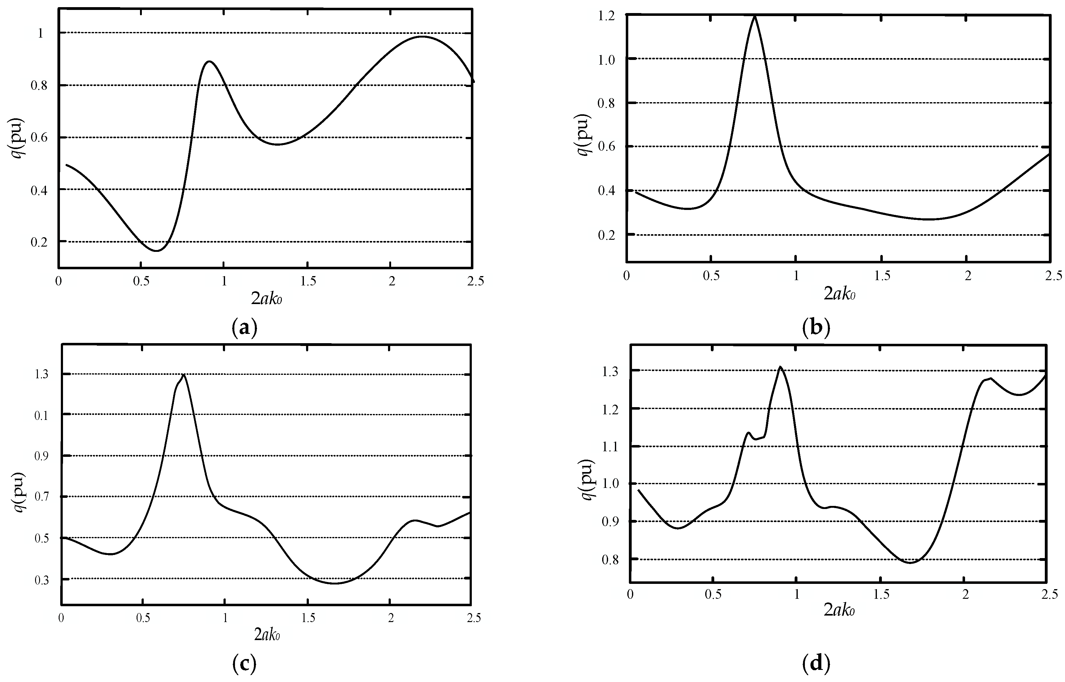
5.1. The Relationship between q and k₀

It was found that the effect of the wave number on q is related to the radius of the float. Thus, set the radius of the float to a constant and the wave number to a variable. The 2ak₀ is exactly the abscissa. Then, calculate the interaction coefficient q to obtain a graph when there are different sizes of float or different float spacings in MATLAB. Furthermore, set the wave number to a variable and the wave number to a constant to repeat the operation above. The optimal value of wave number can be chosen according to the calculation above. Figure 4 shows the relationship between q and k₀.

It can be seen that the value of q will change when the value of wave numbers is different. Optimizing the WEC array is the purpose here. However, it is impossible to optimize the array under each wave number. Figure 4a,b show q under the conditions of the same array size and two floats, but different float spacing, where the float spacing is equal to four times the radius in Figure 4a and eight times the radius in Figure 4b. Figure 4c,d show q under the conditions of the same float spacing and four times the radius, but different array sizes, with three floats in Figure 4c and four floats in Figure 4d. These four subfigures show that a larger q can be obtained in the vicinity of 2ak₀ = 0.8 with arrays of different sizes and float spacings. Therefore, the values of k₀ are fixed with the conditions of 2ak₀ = 0.8 in the next optimization, as shown in Table 1.

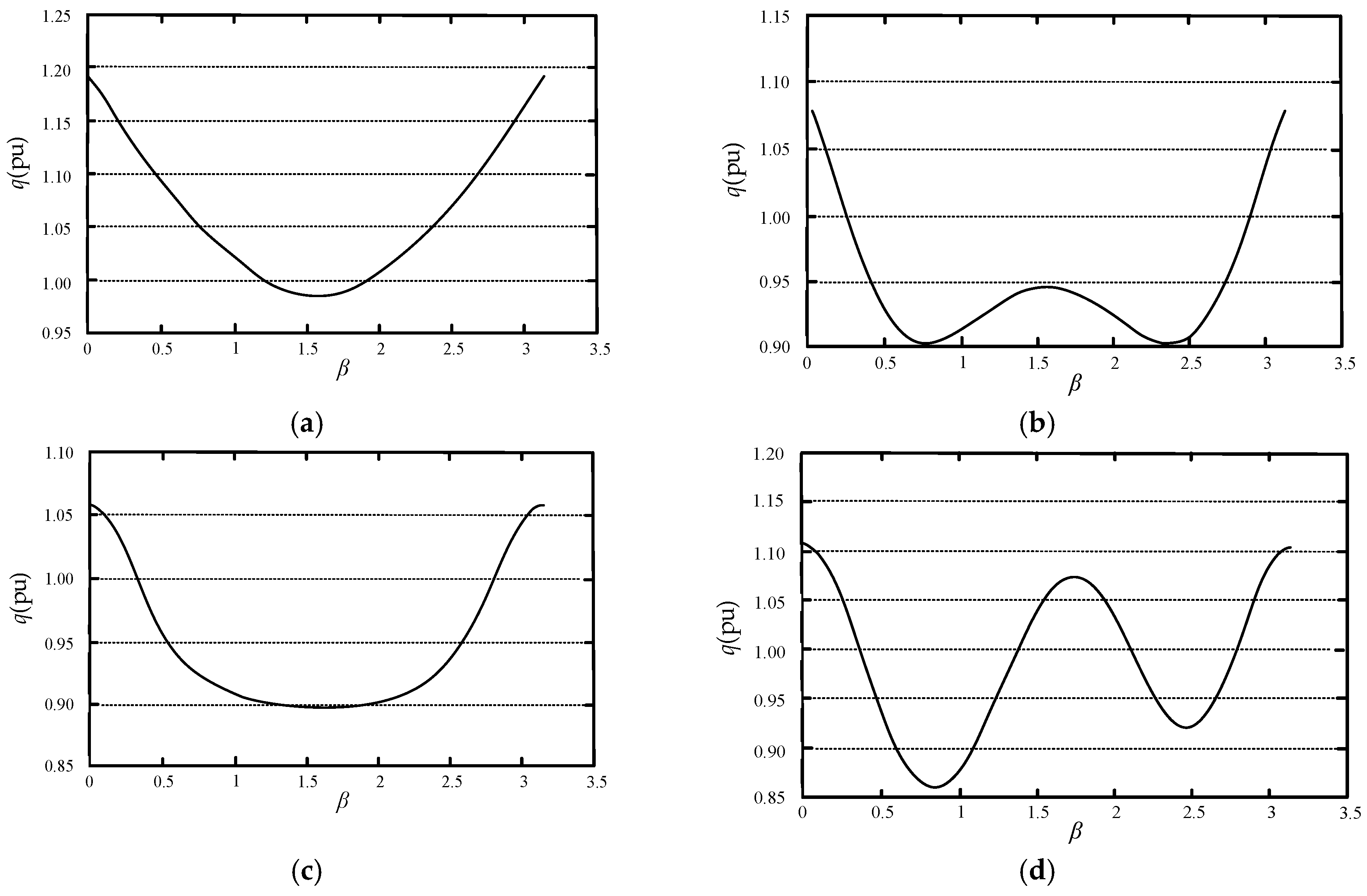
5.2. The Relationship between q and β

Figure 5 shows the influences of the incident angle β on q with different amounts of floats and float spacing. As shown in Figure 5, the q values vary as the incident angle. Figure 5a–d, with the array size and float spacing set the same as in Figure 4, show that, if the array or the float spacing is different, a larger q can be obtained at β = 0. Therefore, β = 0 was selected in the following calculations as shown in Table 1.

Select 2ak₀ = 0.8 and β = 0, and take a two-float array as an example to verify whether the k₀ and β discussed above are correct. As can be seen from Figure 4 and Figure 5, when the float spacing is eight times the radius of the float (5 m), the q is larger than that when float spacing is four times the radius of the float. The two-float array is simple and accurate enough to show the difference. Thus, the two-float array was selected and the float spacing was set to 40 m. Figure 6 presents the corresponding graphics of various velocity potentials.

Figure 6a shows that the values and their distributions of the scattered wave velocity potential of Floats 1 and 2 are different. This indicates that these two floats will affect each other. Figure 6b shows that the velocity potentials of the radiation wave for Floats 1 and 2 are not the same. However, radiation waves are generated by the up and down movement of the float, which shows that the movements of each float are not the same with the interaction between floats. Therefore, it is necessary to calculate the movements of each float. At the same time, the differences between the floats in Figure 6a–c is further proof that the captured energy obtained in the array mode is different from that in isolated mode. This will be further verified with the following calculations.

6. Simulation and Analysis of WEC Arrays

The simulation of WEC arrays is operated in MATLAB. Figure 7 shows a schematic of the array position.

As shown in Figure 7, the position of Float 1 is fixed at the position of (0, 0). The variable that needs to be optimized is the coordinates of the other float. Suppose the size of the array is N. Then there are N − 1 variables that need to be optimized, and the dimension is D = 2 × (N − 1).

The optimal results q depend on the required precision and the parameters of the improved DE algorithm, including the scaling factor, the crossover probability factor, and the size of the population. The required precision is set to 0.001, the range of the scaling factor is between 0.5 to 1, the crossover probability factor is set to 0.9, and the size of the population is set to 10. The given initial positions of the floats cannot influence the optimal layout and output of the WEC arrays. It will only affect the computation speed of the algorithm, whose difference is not so great. For example, if the initial position is closer to the optimal position, the computation speed of the algorithm will be faster and vice versa. The initial conditions are randomly set in the algorithm. Then, during the optimization of array, there will initially be a random population of float positions to determine a better position. It was found that the same optimal layout results can be achieved with different initial conditions.

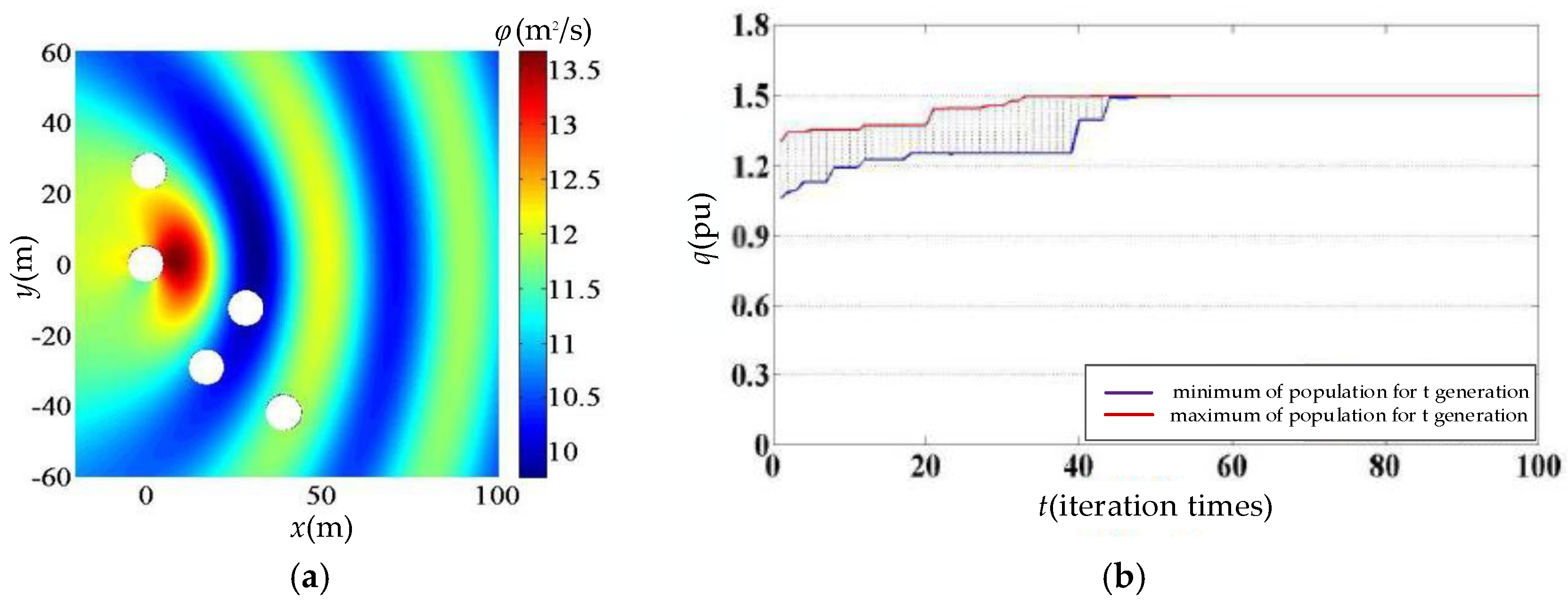
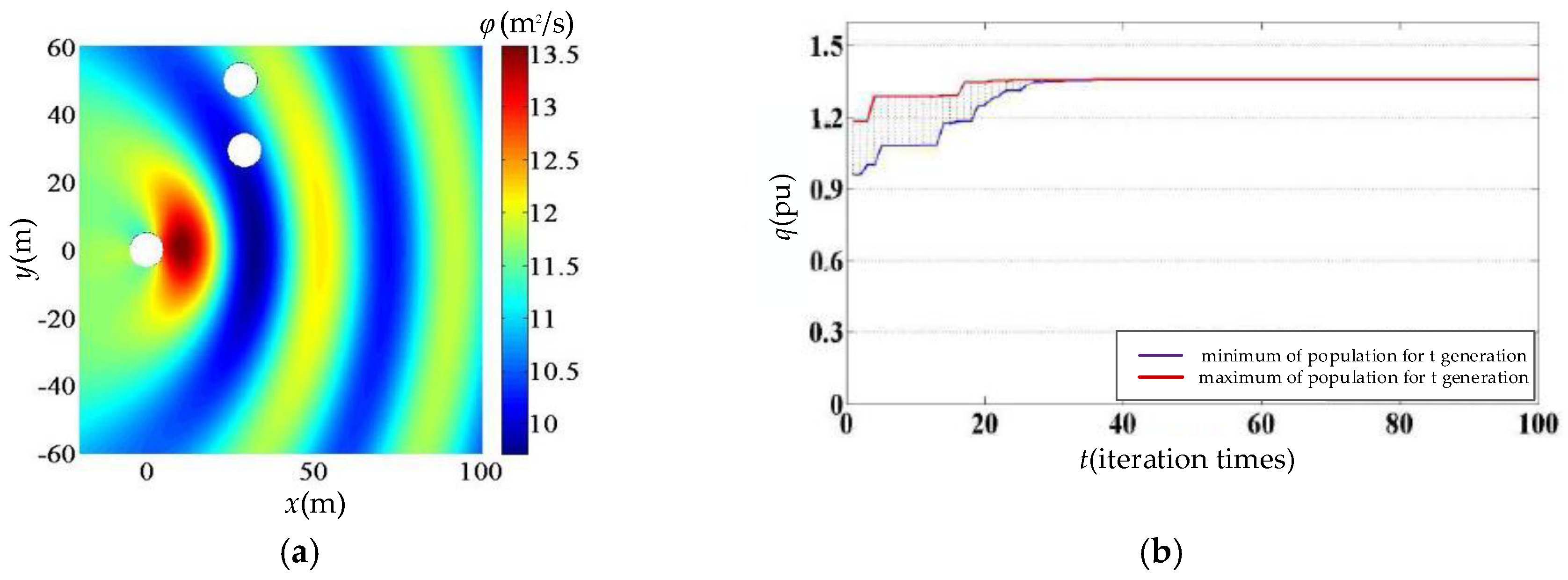
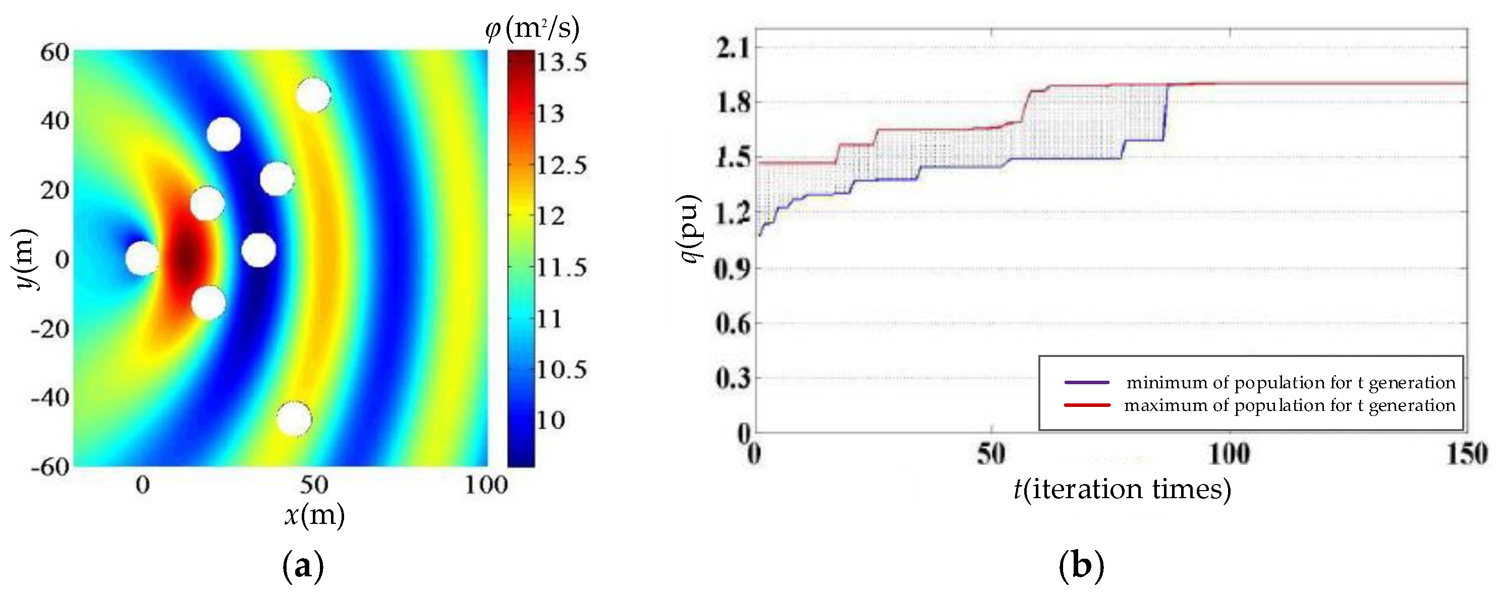
6.1. Simulation of Three-Float, Five-Float, and Eight-Float Arrays

Three typical cases were investigated. Figure 8a shows the optimal result of a simulation of when there are three floats in the sea, and Figure 8b shows the individual fitness values of each generation, which reflects the maximum individual and minimum individual in each group. The blue line reflects the minimum individual in each generation, while the red line reflects the maximum. When the maximum and the minimum individual fitness value in the population is less than the set threshold, that is, when the red line and the blue line in the figure are close to coincidence, the result has converged to its optimal solution.

Table 2. Energy capture coefficient of the WEC array (N = 3).

The Float Number j	Abscissa x (m)	Ordinate y (m)	Interaction Coefficient qj (pu)	Interaction Coefficient q (pu)
1	0	0	1.295	1.358
2	27.895	49.928	1.554
3	29.175	29.323	1.226

shows the energy capture coefficients of the WEC array.

Similarly, a five-float array was optimized. Figure 9a shows the optimal result of the simulation diagram when there are five floats in the sea. Figure 9b shows the individual fitness values of each generation.

Table 3. Energy capture coefficient of the WEC array (N = 5).

The Float Number j	Abscissa x (m)	Ordinatey (m)	Interaction Coefficient qj (pu)	Interaction Coefficient q (pu)
1	0	0	1.408	1.500
2	0.808	26.149	1.673
3	17.149	−29.055	1.459
4	28.355	−12.462	1.438
5	39.021	−41.860	1.524

shows the corresponding energy capture coefficients of the WEC array.

An eight-float array was then optimized. Figure 10 shows the optimal results for the eight-float array.

The optimal position result of each float when there are eight floats in the sea is shown in Figure 10a. The individual fitness values of each generation are shown in Figure 10b.

Table 4. The situation of each float when N = 8.

The Float Number j	Abscissax (m)	Ordinatey (m)	Interaction Coefficient qj (pu)	Interaction Coefficient q (pu)
1	0	0	1.636	1.898
2	18.661	15.639	2.969
3	19.117	−12.829	2.010
4	23.598	35.684	1.817
5	33.668	2.395	3.076
6	38.959	22.869	1.771
7	43.899	−46.321	1.203
8	49.457	46.982	0.706

shows the corresponding energy capture coefficients of the WEC array.

From the optimized WEC arrays with N = 3, N = 5, and N = 8, it can be seen that the larger the array is, the greater the interaction among the floats is. Hence, higher efficiency of the extracted wave energy is achieved. This means that the array composed of multiple floats can extract more wave energy compared with that of the single float operation mode.

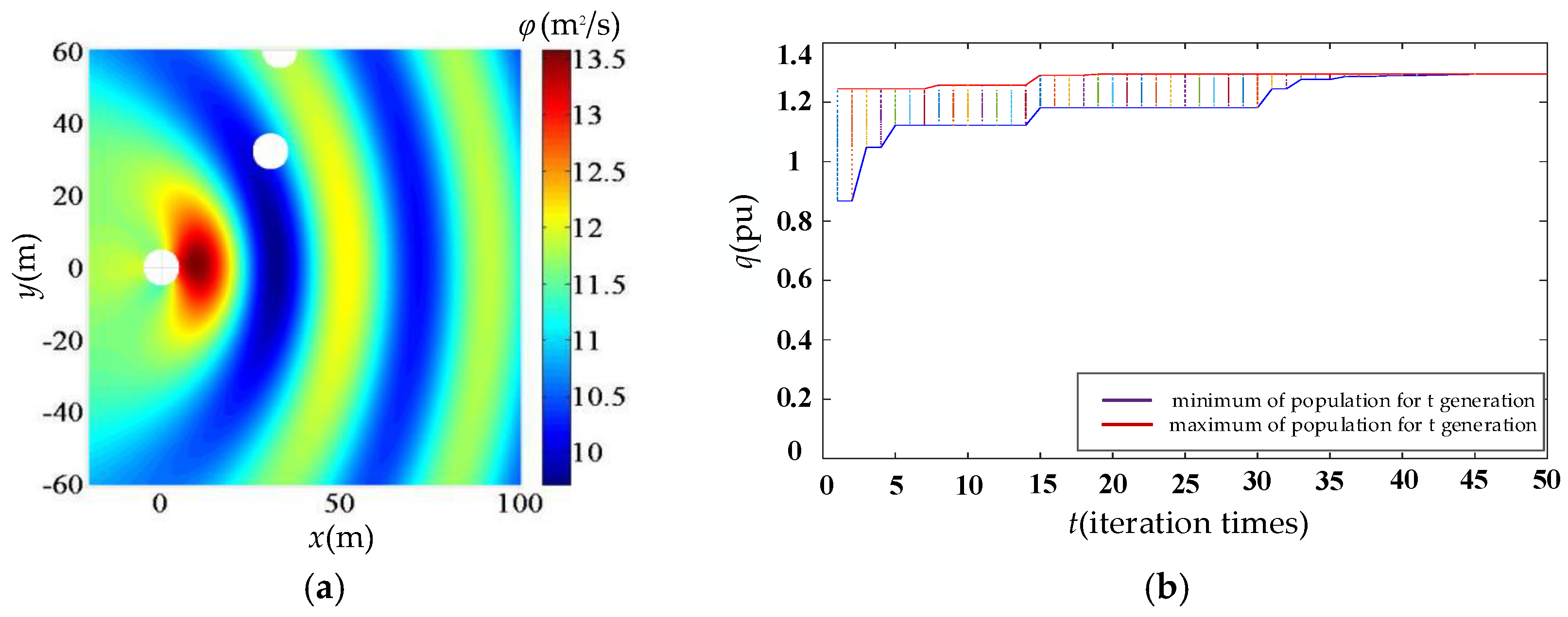
6.2. Comparison with the Traditional DE Algorithm

In order to determine whether the improved DE algorithm is superior to the traditional DE algorithm, a comparison of results for these two algorithms was analyzed. Take a three-float array for example due to its simplicity and representativeness. The optimal position result of each float when there are three floats in the sea is shown in Figure 11a, and the individual fitness values of each generation is shown in Figure 11b.

Table 5. Energy capture coefficient of the WEC array under the traditional DE algorithm (N = 3).

The Float Number j	Abscissax (m)	Ordinate y (m)	Interaction Coefficient qj (pu)	Interaction Coefficient q (pu)
1	0	0	1.220	1.295
2	33.001	60.000	1.505
3	30.401	32.040	1.163

shows the corresponding energy capture coefficients of the WEC array.

Based on the comparison between the improved DE algorithm and traditional DE algorithm, the total energy of the three-float array absorbed from the wave under the traditional DE algorithm is lower than that of the improved DE algorithm. The convergence rate is slower than that of the improved DE algorithm. Furthermore, the program running time of five floats under the improved DE algorithm is about 10 min and about 12 min under the traditional DE algorithm. The program running times of the three floats, under these two algorithms, are both no more than 2 min. If the array is larger, the difference will be more obvious. That is, the improved DE algorithm presented in this paper is effective for the layout optimization of an WEC array. The introduction of an adaptive mutation operator can obtain a better optimal result compared to the traditional DE algorithm.

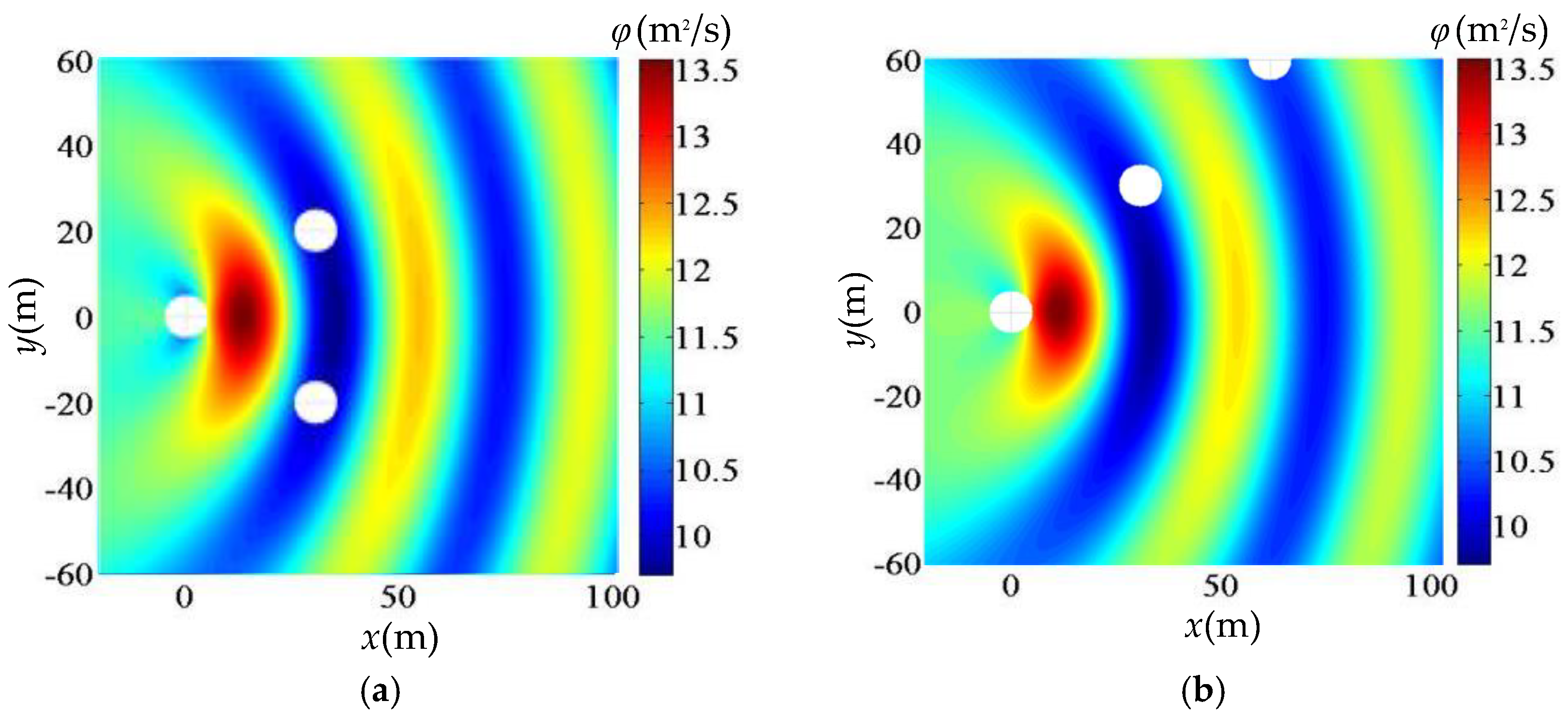
6.3. Comparison with the Homogeneous Distribution of the Three-Float Array

It was found that the optimum of the three cases discussed above is not in a homogeneous distribution. Thus, it deserves further analysis compared with the array under the homogeneous distribution. Take a simple and representative three-float array for example. Three well-distributed arrays are analyzed as follows, whose distance and distribution are slightly similar to the layout results under the algorithm. Figure 12 shows the layout and velocity potential of a homogeneous distribution for a three-float array.

Table 6. Energy capture coefficient of the WEC array (N = 3) under different homogeneous distributions.

Array Layout	The Float Number j	Abscissa x (m)	Ordinate y (m)	Interaction Coefficient qj (pu)	Interaction Coefficient q (pu)
Equicrural triangle	1	0	0	0.894	0.873
	2	30	20	0.862
	3	30	−20	0.862
Straight line	1	0	0	1.216	0.983
	2	30	30	1.044
	3	60	60	0.691

shows the energy capture coefficient of the WEC array (N = 3) under these two typical homogeneous distributions.

It can be seen that the homogeneous distribution cannot improve output compared with the layout calculated by the improved DE algorithm. In Figure 12, the distances between floats of the equicrural triangle layout and the linear layout are similar to the obtained optimal position calculated by the algorithm. However, their interaction coefficients q are far lower than the layout calculated by the algorithm.

7. Discussion

The optimization of a WEC array is of interest for the scientific community. In this paper, a DE algorithm is introduced to optimize a WEC array, by considering the influence of wave radiation and scattering on WEC systems. It was found that the incident angle β and wave number k₀ of the incident wave have a great impact on the output of WEC arrays. Thus, the relationship between these two parameters and q is studied first. It was found that, when β = 0 and the wave number satisfies 2ak₀ = 0.8 (a is the radius of float), a large q will be obtained, which is in proportion to the output power. It is then used to research the layout optimization of WEC arrays later.

The scaling probability factor is then optimized in a differential evolution algorithm in order to make the optimization result more accurate. This is achieved by introducing an adaptive mutation operator to improve the differential evolution algorithm, which yields a faster convergence in the early optimization procedure and, later, a higher precision. The value of the mutation operator will be maintained in the best range for optimization results.

The analysis results show the following:

(1)

When the array is larger, the influence between floats is larger, and more radiation and scattered wave energy can be extracted.

(2)

The total wave energy extracted by WEC arrays is greatly improved compared to that of the single float running mode.

(3)

The optimization of an array under the improved DE algorithm greatly impacts the output of WEC arrays, simultaneously satisfying both convergence precision and speed.

(4)

The optimal layout of the array system is not usually homogeneously distributed. The energy obtained via an inhomogeneous array distribution is greater than that of a homogeneous distribution.

(5)

With the introduction of an adaptive mutation operator, the layout optimization of WEC arrays is superior to that of a constant mutation operator.

Noted that this model was studied under a regular wave, whose array arrangement law may be different from that of an irregular wave. However, this can be neglected because there is little difference in practical engineering. In addition, the damping of a generator can also be considered with this model. Therefore, WEC arrays optimized by the improved DE algorithm have great potential for development.

References

1. Yan, Y.B. Principle and Device of the Ocean Wave Energy Conversion Generation, 1st ed.; Shanghai Scientific & Technical Publishers: Shanghai, China, 2013; ISBN 978-7-5478-1527-4. [Google Scholar]
2. Twidell, J.; Weir, A.D. Renewable Energy Resources, 2nd ed.; Taylor and Francis: London, UK, 2006; ISBN 978-0-4192-5320-4. [Google Scholar]
3. Chu, H.M. Control of Wave Power Generation Arrays with Modular Multilevel Converter. Master’s Thesis, Tianjin University, Tianjin, China, 2014. [Google Scholar]
4. Cheng, Y.L.; Dang, Y.; Wu, Y.J. Status and Trends of the Power Generation from Wave. Appl. Energy Technol. 2009, 12, 26–30. [Google Scholar]
5. Dalton, G.J.; Alcorn, R.; Lewis, T. Case study feasibility analysis of the pelamis wave energy convertor in Ireland, Portugal and North America. Renew. Energy 2013, 35, 443–455. [Google Scholar] [CrossRef]
6. He, G.Y.; Yang, S.H.; He, H.Z.; Wang, F.Y. Hydrodynamic analysis of array-type device of wave energy generation. J. Hydroelectr. Eng. 2015, 34, 118–124. [Google Scholar]
7. Zhang, Y.; Lin, Z. Advances in ocean wave energy converters using piezoelectric materials. J. Hydroelectr. Eng. 2011, 30, 146–148. [Google Scholar]
8. Han, B.F.; Chu, J.K.; Xiong, Y.S.; Yao, F. Progress of research on ocean energy power generation. Power Syst. Clean Energy 2012, 28, 61–65. [Google Scholar]
9. Budal, K. Theory for absorption of wave power by a system of interacting bodies. J. Ship Res. 1977, 21, 248–253. [Google Scholar]
10. Mavrakos, S.A.; Kalofonos, A. Power absorption by arrays of interacting vertical axisymmetric wave-energy devices. J. Offshore Mech. Arct. Eng. 1997, 119, 244–250. [Google Scholar] [CrossRef]
11. Yilmaz, O. Hydrodynamic interactions of waves with group of truncated vertical cylinders. J. Waterw. Port Coast. Ocean Eng. 1998, 124, 272–279. [Google Scholar] [CrossRef]
12. Yilmaz, O.; Incecik, A. Analytical solutions of the diffraction problem of a group of truncated vertical cylinders. Ocean Eng. 1998, 25, 385–394. [Google Scholar] [CrossRef]
13. Garrett, C.J.R. Wave forces on a circular dock. J. Fluid Mech. 1971, 46, 129–139. [Google Scholar] [CrossRef]
14. Kagemoto, H.; Yue, D.K.P. Interactions among multiple three-dimensional bodies in water waves: An exact algebraic method. J. Fluid Mech. 1986, 166, 189–209. [Google Scholar] [CrossRef]
15. Child, B.F.M.; Venugopal, V. Optimal configurations of wave energy device arrays. Ocean Eng. 2010, 37, 1402–1417. [Google Scholar] [CrossRef]
16. Blanco, M.; Moreno, T.; Lafoz, M.; Ramírez, D. Design Parameter Analysis of Point Absorber WEC via an Evolutionary-Algorithm-Based Dimensioning Tool. Energies 2015, 8, 1203–11233. [Google Scholar] [CrossRef]
17. Bozzi, S.; Bizzozero, F.; Gruosso, G.; Passoni, G.; Giassi, M. Analysis of interaction of point absorbers’ arrays for seawave electrical energy generation in italian seas. In Proceedings of the 2016 International Symposium on Power Electronics, Electrical Drives, Automation and Motion (SPEEDAM), Anacapri, Italy, 22–24 June 2016; pp. 1369–1374. [Google Scholar]
18. Mercadé Ruiz, P. Hydrodynamic Modelling and Layout Optimisation of Wave Energy Converter Arrays. Ph.D. Thesis, Aalborg University, Aalborg, Denmark, 2017. [Google Scholar]
19. Ferri, F. Computationally efficient optimisation algorithms for WECs arrays. In Proceedings of the 12th EWTEC-Proceedings of the 12th European Wave and Tidal Energy Conference, Cork, Ireland, 27 August–1 September 2017; pp. 1–7. [Google Scholar]
20. Verbrugghe, T.; Stratigaki, V.; Troch, P.; Rabussier, R.; Kortenhaus, A. A Comparison Study of a Generic Coupling Methodology for Modeling Wake Effects of Wave Energy Converter Arrays. Energies 2017, 10, 1697. [Google Scholar] [CrossRef]
21. Mercadé Ruiz, P.; Nava, V.; Mathew, B.R.T.; Ruiz Minguela, P.; Ferri, F.; Peter Kofoed, J. Layout Optimisation of Wave Energy Converter Arrays. Energies 2017, 10, 1262. [Google Scholar] [CrossRef]
22. Thomas, S.; Eriksson, M.; Göteman, M.; Hann, M.; Isberg, J.; Engström, J. Experimental and Numerical Collaborative Latching Control of Wave Energy Converter Arrays. Energies 2018, 11, 3036. [Google Scholar] [CrossRef]
23. Balitsky, P.; Verao, F.G.; Stratigaki, V.; Troch, P.; Troch, P. Assessment of the Power Output of a Two-Array Clustered WEC Farm Using a BEM Solver Coupling and a Wave-Propagation Model. Energies 2018, 11, 2907. [Google Scholar] [CrossRef]
24. OceanEd. Available online: https://github.com/D-Forehand/OceanEd/ (accessed on 1 December 2018).
25. Forehand, D.I.M.; Kiprakis, A.E.; Nambiar, A.J.; Wallace, A.R. A fully coupled wave-to-wire model of an array of wave energy converters. IEEE Trans. Sustain. Energy 2016, 7, 118–128. [Google Scholar] [CrossRef]
26. Wang, D. Study of the Combined Oscillating Buoys’ Layout. Master’s Thesis, Ocean University of China, Qingdao, China, 2015. [Google Scholar]
27. Fang, H.W.; Chen, Y.; Hu, X.L. Wave Power Generation and its Control. J. Shenyang Univ. 2015, 27, 376–384. [Google Scholar]
28. Bangmin, Z. Computational Hydrodynamics, 1st ed.; Wuhan University Press: Wuhan, China, 2001; ISBN 7-307-03296-1. [Google Scholar]
29. Fang, H.W.; Cheng, J.J.; Ren, Y.Q. Force analysis of float-type wave energy converter. J. Tianjin Univ. 2014, 47, 446–451. [Google Scholar]
30. Mercadé Ruiz, P.; Ferri, F.; Kofoed, J.P. Experimental validation of a wave energy converter array hydrodynamics tool. Sustainability 2017, 9, 115. [Google Scholar] [CrossRef]
31. Child, B.F.M. On the Configuration of Arrays of Floating Wave Energy Converters. Ph.D. Thesis, Edinburgh University, Edinburgh, UK, 2011. [Google Scholar]
32. Abramowitz, M.; Stegun, I.A. Handbook of Mathematical Functions, 1st ed.; Government Printing Office: Washington, DC, USA, 1964. [Google Scholar]
33. Kagemoto, H.; Yue, D.K.P. Hydrodynamic interaction analyses of very large floating structures. Mar. Struct. 1993, 6, 295–322. [Google Scholar] [CrossRef]
34. Evans, D.V. Some Analytic Results for Two and Three Dimensional Wave- Energy Absorbers. Power from Sea Waves; Academic Press, Inc.: London, UK, 1980; pp. 213–249. [Google Scholar]
35. Zhou, Y.P.; Gu, X.S. Development of Differential Evolution Algorithm. Control. Instruments Chem. Ind. 2007, 34, 1–5. [Google Scholar]
36. Wu, L.H. The Research and Applications of Differential Evolution Algorithm; Hunan University: Hunan, China, 2007. [Google Scholar]
37. Liu, B.; Wang, L.; Jin, Y.H. Advances in differential evolution. Control Decis. 2007, 22, 721–729. [Google Scholar]
38. Gao, Y.L.; Liu, J.M. Parameter study of differential evolution algorithm. J. Nat. Sci. Heilongjiang Univ. 2009, 26, 81–85. [Google Scholar]
39. Yang, Z.Y.; Tang, K. An overview of parameter control and adaptation strategies in differential evolution algorithm. CAAI Trans. Intell. Syst. 2011, 6, 415–423. [Google Scholar]
Figure 1. Float-type wave energy converter (WEC): (a) front view; (b) side view.
Energies 11 03522 g001
Figure 2. Simplified diagram of the float in wave.
Energies 11 03522 g002
Figure 3. The two-float WEC array.
Energies 11 03522 g003
Figure 4. The relationship between q and k0: (a) N = 2, L = 4a; (b) N = 2, L = 8a; (c) N = 3, L = 8a; (d) N = 4, L = 8a.
Energies 11 03522 g004
Figure 5. The relationship between q and β: (a) N = 2, L = 4a; (b) N = 2, L = 8a; (c) N = 3, L = 8a; (d) N = 4, L = 8a.
Energies 11 03522 g005
Figure 6. Velocity potential: (a) scattered wave velocity potential of Float 1 (left) and Float 2 (right); (b) radiation wave velocity potential of Float 1 (left) and Float 2 (right); (c) the velocity potential of Float 1 (left) and Float 2 (right).
Energies 11 03522 g006
Figure 7. A schematic of the array position.
Energies 11 03522 g007
Figure 8. Optimal results for the three-float array: (a) the optimal position; (b) individual fitness values for each generation.
Energies 11 03522 g008
Figure 9. Optimal results for the five-float array: (a) the optimal position; (b) individual fitness values for each generation.
Energies 11 03522 g009
Figure 10. Optimal results for the eight-float array: (a) the optimal position; (b) individual fitness values for each generation.
Energies 11 03522 g010
Figure 11. Optimal results for the three-float array under the traditional DE algorithm: (a) the optimal position; (b) individual fitness values for each generation.
Energies 11 03522 g011
Figure 12. Layout and velocity potential of homogeneous distribution for the three-float array: (a) equicrural triangle; (b) straight line.
Energies 11 03522 g012