Abstract
The life-cycle cost reduction of medium-class gas turbine power plants was investigated using the mathematical optimization technique. Three different types of gas turbine power cycles—a simple cycle, a regenerative cycle, and a combined cycle—were examined, and their optimal design conditions were determined using the sequential quadratic programming (SQP) technique. As a modeling reference, the Siemens SGT-700 gas turbine was chosen and its technical data were used for system simulation and validation. Through optimization using the SQP method, the overall costs of the simple cycle, regenerative cycle, and combined cycle were reduced by 7.4%, 12.0%, and 3.9%, respectively, compared to the cost of the base cases. To examine the effect of economic parameters on the optimal design condition and cost, different values of fuel costs, interest rates, and discount rates were applied to the cost calculation, and the optimization results were analyzed and compared. The values were chosen to reflect different countries’ economic situations: South Korea, China, India, and Indonesia. For South Korea and China, the optimal design condition is proposed near the upper bound of the variation range, implying that the efficiency improvement plays an important role in cost reduction. For India and Indonesia, the optimal condition is proposed in the middle of the variation ranges. Even for India and Indonesia, the fuel cost has the largest contribution to the total cost, accounting for more than 60%.
1. Introduction
World electricity consumption is increasing continuously; the 3240 TWh of total electricity consumption in 1971 increased to 9310 TWh in 2013 [1]. This substantial increase was propelled by economic growth and the increasing desire for high-quality energy. In many developed countries, electricity is produced at centralized, large-scale power plants [2], such as coal-fired, nuclear, and gas turbine power plants. According to energy statistics [3], coal, natural gas, and nuclear fuels account for 41.3%, 21.7%, and 10.6% of the total electricity generated of the world, respectively. To meet the increasing demand for electricity, power generation capacity must be increased, either by enlarging the existing power plants or constructing new ones. However, neither of these options is typically accepted by the public, particularly if the power plants are located near their residential areas [4].
As an alternative to large-scale, centralized power plants, small-scale power plants located at or near the consumer sites can supply electricity; these small power generators are called distributed (or decentralized) power generation (DPG). The use of DPG is increasing; it was responsible for 21% of the global electricity generation in 2000, and it is projected to account for approximately 40% of the global electricity increase in 2020 [5].
Among several available technologies such as photovoltaic panels, wind turbines, internal combustion engines, and fuel cells [6,7], gas turbines were recognized as the most attractive option from the technological and economic standpoints [5]. However, power generation using small- or medium-sized gas turbines still remains expensive compared to the large-scale power generators [8] due to the relatively higher investment costs and lower electrical efficiencies. Therefore, reducing the operating costs of gas turbines by means of the mathematical optimization is crucial, particularly in distributed power generation areas. As shown in Table 1, several commercial gas turbine products exist that are suitable for use in large factories and urban buildings [8,9,10,11].

Table 1.
Technical data of medium-sized commercial gas turbine models [8,9,10,11].
Many analyses on gas turbine power cycles were conducted, for example, by Kurt et al. [12] and Ahmadi et al. [13]. Kurt et al. [12] calculated and compared the net power output and thermal efficiency of an open-cycle gas turbine with various designed conditions for the compressor inlet temperature, turbine inlet temperature/pressure ratio, and compressor and turbine isentropic efficiencies. Ahmadi et al. [13] evaluated a gas turbine regenerative cycle through an exergoeconomic analysis, and applied multi-objective optimization to obtain the maximum exergy efficiency and minimum cost. They concluded that increasing compressor and turbine efficiencies and increasing the air preheating temperature considerably impact efficiency improvement and cost reduction.
Along with system simulation and economic analysis, mathematical optimization was applied to gas turbine power cycles [14,15,16,17,18]. For the optimization, several algorithms were selected depending on the type of optimization, e.g., the mixed integer linear programming (MINLP), genetic algorithm (GA), simplex method, and sequential quadratic programming (SQP). MINLP is typically used for problems with discrete variable sets and nonlinear functions [19], GA is preferred for finding multiple optimal points [20], and the simplex method is recommended for overcoming the problem of local solutions, indeterminacies, and discontinuities [21]. The SQP method is one of the most recently developed optimization algorithms [22], and possibly one of the most effective and computationally inexpensive methods [23]. Given these advantages, the method was applied to the optimization of energy systems, for example, supercritical coal-fired power plants [24], ion transfer membrane oxy-combustion systems [25], cogeneration systems [26], and solid oxide fuel cell power generation [27]. However, the SQP method is yet to be applied to gas turbine-based power plants.
In gas turbine power generation, the fuel cost contributes the most to the overall cost. Therefore, previous optimization studies on gas turbines [12,13] focused on efficiency improvement even though the improvement would increase the capital investment. However, the price of natural gas recently dropped primarily due to the production of shale gas. In this context, capital investment and fuel cost now differently contribute to the overall cost; trade-off comparison and optimization improve the cost efficacy of gas turbines.
In this study, we applied the SQP method to gas turbine-based power cycles with the aim of minimizing the life-cycle cost of electricity generation. Through optimization, a new set of design conditions for each gas turbine power cycle is proposed. Case studies were also carried out, investigating the effects of economic parameters, such as fuel price, interest rate, and escalation rate, on the optimal conditions and life-cycle cost of gas turbine power cycles. During optimization, the levelized annual cost rate was chosen as the objective function to be minimized. To calculate the life-cycle costs, initial capital costs, fuel costs, and maintenance costs were considered over the lifetime of the power plants. As a first step of the analysis, gas turbine power cycles were modeled and the energy/mass balances were calculated. Using the energy/mass balance data and appropriate economic assumptions, the levelized cost of electricity was calculated. Finally, a new design condition for each gas turbine power cycle was suggested using the SQP optimization technique; through the appropriate selection of design conditions, the lowest life-cycle cost was achieved. For the system simulation, a commercial software package Aspen Plus® (Bedford, MA, USA) [28] was used and the built-in SQP algorithm was employed in the cost optimization.
2. Analyzed Power Cycles and Their Performance Modeling
2.1. Description of Cycle Configurations
A gas turbine simple cycle, regenerative cycle, and combined cycle are depicted in Figure 1a–c, respectively. As a simulation basis, we selected the Siemens SGT-700 (Siemens Aktiengesellschaft, Munich, Germany) since it is the most electrically efficient among the commercial gas turbines products listed in Table 1. The design parameters and technical data of the SGT-700 were obtained from a technical handbook [8] and Hellberg et al. [11]. The SGT-700 generates 32.8 MW of electricity and has a 36.9% electrical efficiency.
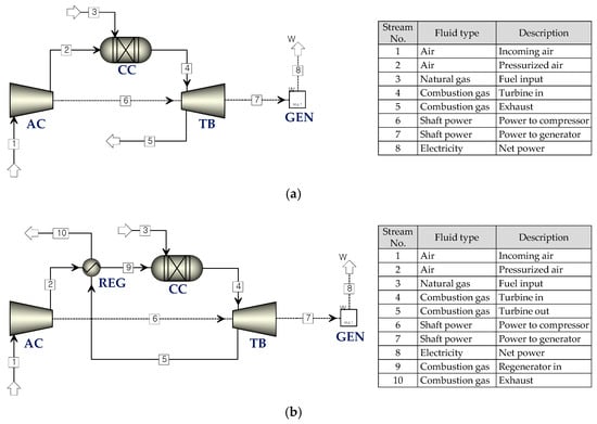
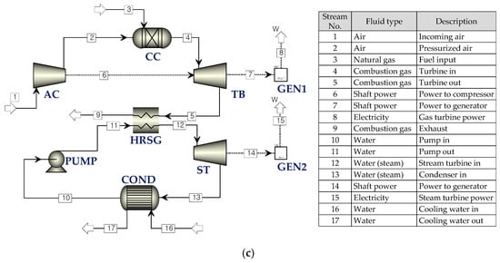
Figure 1.
Flow diagrams of gas turbine power cycles: (a) gas turbine simple cycle; (b) gas turbine regenerative cycle; (c) gas turbine combined cycle. Abbreviations are defined as AC: air compressor, CC: combustion chamber, TB: turbine, GEN: generator, REG: regenerator, HRSG: heat recovery steam generator, ST: steam turbine, and COND: condenser.
In the gas turbine simple cycle, the air is compressed by an air compressor (AC) and enters the combustion chamber (CC) as an oxidizer for the combustion reaction. The natural gas, stream number 3, is supplied to the CC as a fuel. Then, the high-pressure and high-temperature combustion gas drives the turbine (TB), generating electrical power in the generator (GEN).
In the regenerative cycle depicted in Figure 1b, thermal energy is internally recovered from the turbine exiting stream to the compressor outgoing air stream at the regenerator (REG), enhancing the thermal efficiency of the overall system. The technical data of the SGT-700 were also applied to the regenerative cycle, except for the discharge pressure of the turbine; a slightly higher value was assumed to consider the pressure loss of the regenerator. The effectiveness of the regenerator was assumed to be 75%, and the pressure drops at the air side and exhaust gas side were assumed to be 2% and 5% of the incoming pressures, respectively.
Figure 1c diagrams the flow of the gas turbine combined-cycle that consists of a gas turbine, a heat recovery steam generator (HRSG), a steam turbine (ST), a condenser (COND), and a water pump (PUMP). Steam is produced by recovering thermal energy, which then drives a steam turbine, generating additional power. In this study, a single-pressure steam cycle was assumed. The assumptions and detailed information on the gas turbine combined-cycle were collected from previous studies [8,11,29].
2.2. System Simulation
As mentioned above, Aspen Plus® (Aspen Technology, Bedford, MA, USA) [28] was used to calculate the energy/mass balance. Table 2 summarizes the simulation method within Aspen Plus® and Table 3 presents the detailed information of the equipment modeling. For all simulations, we assumed that there was no pressure drop on the pipe connection, along with a complete combustion for combustor, and no heat losses on the equipment or pipe connection. In the property calculation, the ideal gas equation was used and steam table information was used for the water side.
Table 2.
Model description of analyzed power cycles in Aspen Plus®.
Table 3.
Detailed technical data for simple, regenerative, and combined gas turbine cycles [11,29].
3. Optimization
3.1. Optimization Algorithm
The SQP method is recognized as one of the most effective optimization techniques for solving constrained nonlinear optimization problems [23]. As shown in Figure 2, SQP solves the nonlinear problems through linear approximation. By using Newton’s method, a quadratic sub-problem is generated, which is easier to solve.
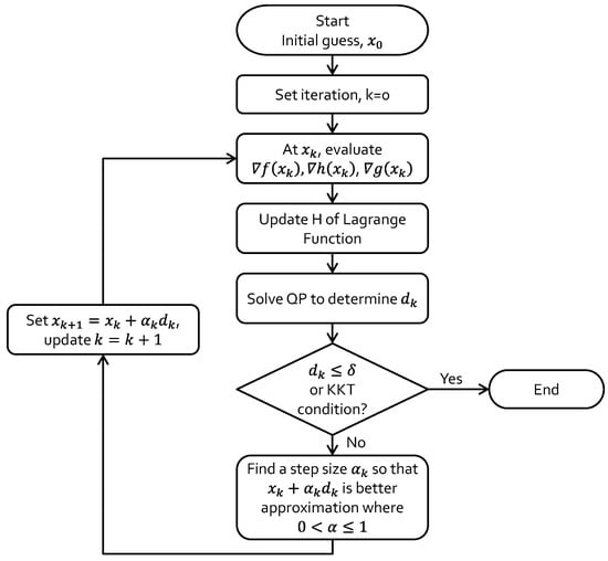
Figure 2.
Calculation procedure of sequential quadratic programming (SQP) method [31,32,33].
Nonlinear optimization problems are typically expressed by Equations (1)–(3), determining the value of matrix X that minimizes the object function f(X), subject to the equality and inequality constraints.
subject to the following:
The Lagrangian function of this problem, L(X, λ, μ), can be expressed as
where λ and μ are vectors of multipliers for equality and inequality constraints, respectively.
The quadratic sub-problem is constructed by linearizing the constraints, and can be written as
subject to the following:
Solving Equations (5)–(7) results in a solution vector d with multiplier vectors λ and μ, defined as , , and , respectively. This quadratic result creates a search direction for X and calculates the acceptable estimates for the Karush–Kuhn–Tucker (KKT) multipliers and H. The H in Equation (5) is a positive definite Hessian matrix of the Lagrangian function, which is updated by the Broyden–Fletcher–Goldfarb–Shanno method, which calculates the second derivatives of the objective function and constraint functions. The solution converges when the vector d is less than the relative tolerance (δ) of 0.0001, and when the KKT conditions are satisfied [28,32,33]. A step size α is chosen to ensure the decrease in the objective function [34]. The procedure described above is iterated until the solution X* is obtained. A more detailed description about the SQP algorithm is provided in previous studies [22,23,31,32,33].
As described in Section 1, the optimization algorithm is already included in the Aspen Plus® software, in which the system was simulated; therefore, the optimization could be easily and inexpensively completed. The optimization problem for the gas turbine simple cycle was defined as shown in Equation (8), targeting minimum life-cycle cost rate () of the power cycle during the entire lifetime.
3.2. Calculation of Life-Cycle Cost
Each company or institution has its own preferred method of economic analysis. The net present value (NPV) method, internal rate of return (IRR) method, or benefit/cost (B/C) ratio method can be used depending on the characteristics of the economic problems [34]. In the economic evaluation of a power plant or an energy conversion system, life-cycle consideration was recommended [35,36]; all the costs occurring during the entire lifetime of the plant are considered. Both the initial capital cost, primarily caused by the equipment purchasing, and the operational cost, mainly associated with the fuel use and regular maintenance of the plant, should be investigated. For more accurate analysis, return on investment, taxes, and insurance can be included. In this study, we followed the procedure of economic analysis proposed by Bejan et al. [37]; however, for simple analysis and clear comparison, only the equipment costs, fuel costs, and operation and maintenance (O&M) costs were included.
The purchased equipment cost (PEC) of each component Zk was estimated using the cost equations, which were collected from different literature sources [16,38,39,40]. The constants used in the cost equations were adjusted in this study to create a good agreement between the estimated values and the current market price of gas turbines. The comparison results are shown in Figure 3. Detailed information of the cost equations and the constants are summarized in Table A1 and Table A2 (Appendix A).
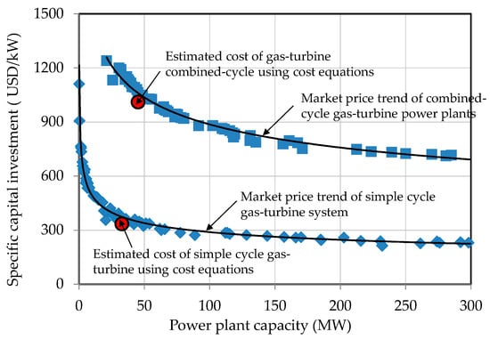
Figure 3.
Comparison between the cost estimate and the current market price [8] of gas turbines.
The estimated value of PEC for each component was updated to the value of the reference year using the cost index. The reference year was assumed to be 2013 and the Chemical Engineering Plant Cost Indices (CEPCI) [41] were used for the cost update. Notably, correction factor (R) of 3.0 was employed for the combined cycle to incorporate the cost of balance of plant (BOP) and plant construction [42].
The cost rate of equipment purchasing () and O&M () were calculated using Equations (9) and (10), respectively [37], covering the entire lifetime of the plant (n). The capital recovery factor (CRF) was used for cost distribution, which is a function of the effective interest rate (ieff) and lifetime (n), as shown in Equation (11). The constant-escalation leveling factor (CELF) was calculated using Equations (12) and (13), where k and rn are the levelization factor and nominal escalation rate, respectively. More detailed information of the cost calculation can be found in Bejan et al. [37].
In the calculation of the fuel cost rate (), the CELF was also used, as shown in Equation (14). , , and LHV are the fuel flow rate, specific cost of fuel, and lower heating value of fuel, respectively.
In this study, the unit cost of fuel () was assumed to be $17.24 United States dollars (USD) per GJ, reflecting the natural gas price in South Korea in 2015 [3]. Natural gas prices fluctuate considerably year to year; the effect of the fuel cost on the overall cost was investigated in this study, and is discussed in Section 4.5. The nominal specific capital investment (), expressed in USD/kW, was calculated using Equation (15). The overall cost rate () was calculated using Equation (16), which is an objective function to be minimized through optimization. Finally, the levelized cost of electricity (LCOE), expressed in USD/MWh, was calculated using Equation (17). Table 4 summarizes the assumptions and values used in the cost calculations.
Table 4.
Primary assumptions and values used in cost calculations. O&M—operation and maintenance; USD—United States dollar.
3.3. Optimization Procedure
Table 5 summarizes the equality and inequality constraints and the range of decision variables. During the optimization, the equality constraints were kept constant; for instance, the net power output () and turbine inlet temperature () were fixed for the gas turbine simple cycle, regardless of the change in other design variables. To keep the net power output and turbine inlet temperature constant, the air flow rate () and the fuel flow rate () were recalculated.
Table 5.
Constraints and range of decision variables in mathematical optimization.
The inequality constraints were selected considering the technological status of the gas turbine components [18,38,39,44]. As discussed in Section 4.2 and shown in Table A1, design variables, such as the air compressor pressure ratio, compressor and turbine isentropic efficiencies, were included in the cost equations. These values were also used as variables during optimization.
For the gas turbine simple cycle, the air compressor pressure ratio (), isentropic efficiency of compressor (), and the isentropic efficiency of the turbine () were chosen for the variables and inequality constraints. In the gas turbine combined cycle, the drum saturation pressure (), the outlet temperature of the economizer (), and the outlet temperature of the superheater () were adjusted to 15–45 bar, 170–230 °C, and 127–600 °C, respectively, satisfying the pinch-point temperature difference at the evaporator, and the approach temperatures of the superheater and economizer. The flow rate of circulating water () also varied within 700–2000 kg/s to maintain the condenser outlet temperature.
4. Results and Discussion
4.1. Validation of the System Simulation
Table 6 compares the simulation results and the technical data of the SGT-700, showing good mutual agreement. The calculation error ranged from 0.46 to 2.77%, except for the turbine exhaust temperature. Therefore, the simulation model was confirmed and used during the following cost optimization step.
Table 6.
Comparison of technical data and simulation results for gas turbine simple cycle.
Table 7 compares the simulation results of the combined cycle and the technical data of the SCC-700 power plant [8,11], showing the good agreement of the data, with maximum error of 0.5%. Therefore, during the optimization of the combined cycle, the simulation model was also used. In the system simulation of the combined cycle, we assumed the bottoming steam cycle was a single-pressure steam cycle; therefore, the electrical efficiency of the simulation was calculated to be slightly lower than the design efficiency of the SCC-700 plant.
Table 7.
Comparison of technical data and simulation results for gas turbine combined cycle. N/A—not applicable.
4.2. Optimization Results and Cost Reduction for the Gas Turbine Simple Cycle
Table 8 summarizes the optimization results of the gas turbine simple cycle, where a new set of design conditions was proposed by the SQP algorithm. As shown in the table, the new design conditions increase efficiencies and equipment cost. As a result, the nominal specific capital investment almost doubles, from 335.1 USD/kW up to 629.3 USD/kW.
Table 8.
Optimized results and relevant cost calculations for gas turbine simple cycle. LCOE—levelized cost of electricity.
To investigate how the decision variables affect the cost rate, a sensitivity analysis was performed and the results are presented in Figure 4. As shown in Figure 4, the overall cost rate exhibits a concave pattern with respect to the change of the compressor pressure ratio. In this calculation, the sets of efficiencies of the compressor and turbine were arbitrarily chosen to determine the effect of the efficiencies on the cost.
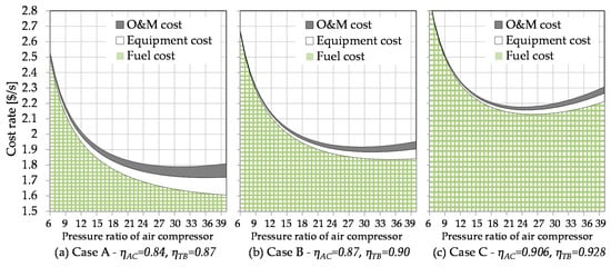
Figure 4.
Cost rates of gas turbine simple cycle with respect to change of compressor pressure ratio for various compressor and turbine efficiencies: (a) isentropic efficiencies of air compressor and turbine were assumed to be 84% and 87%, respectively; (b) 87% and 90%; (c) 90.6% and 92.8%.
As described in Section 3.3, the maximum pressure ratio was limited to 25 in this study, and the optimum value was determined at 24.9, very close to the upper bound. If the pressure ratio limit was set higher, e.g., 40, the optimum value would shift to a greater pressure ratio, as depicted in Figure 3b,c. At lower compressor and turbine efficiencies, such as the case shown in Figure 3a, the overall cost rate of the system was calculated to be greater than the more efficient cases. As shown in Figure 3a–c, the fuel cost dominates the overall cost and the contribution of the fuel cost becomes more dominant for the less efficient cases.
4.3. Optimization Results and Cost Reduction for the Gas Turbine Regenerative Cycle
Table 9 compares the design condition of the base case and the optimized case for the gas turbine regenerative cycle. In the calculation, the same technical data, which were used in the gas turbine simple cycle, were used. The net power output and turbine inlet temperature remained fixed at 32.63 MW and 1145 °C, respectively. As described in Section 2.2, due to the internal energy recovery, the electrical efficiency was more efficient, at 38.3%, which is a 1.59%-point increase compared to the gas turbine simple cycle. However, the specific capital investment increased by 25.6%, from 335.1 USD/kW to 421.0 USD/kW, primarily due to the installation of the regenerator.
Table 9.
Optimization results and relevant cost calculation for regenerative cycle.
In the optimized case of the regenerative cycle, the pressure ratio of the air compressor was suggested to be a small value of 8.16, which is close to the lower boundary. In this condition, the energy recovery at the regenerator can be maximized, implying that the internal energy recovery at the regenerator plays an important role in cost minimization. The efficiencies of compressor and turbine were proposed in the middle of the variation range, at the most cost-effective value. The specific capital investment marginally increased from 421.0 USD/kW to 422.54 USD/kW.
In the regenerative cycle, the effectiveness of the regenerator has a large impact on the electrical efficiency, as well as on the fuel use. For the base case, the effectiveness was assumed to be 75%. However, after optimization, the effectiveness was set to 80%—the upper limit of the variation range. In Figure 5, the changing trends in the overall cost rate with respect to the change in pressure ratio are presented for various regenerator effectiveness values. As the effectiveness increased, the temperature difference between the turbine outlet and compressor outlet streams increased; consequently, more thermal energy can be recovered and the electrical efficiency of the overall system improves. Necessarily, the greater effectiveness of the regenerator results in a higher purchased equipment cost, but its contribution is relatively small.
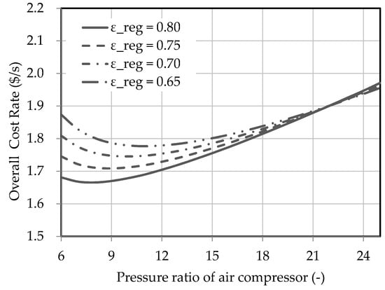
Figure 5.
Overall cost rates for the gas turbine regenerative cycle for various regenerator effectiveness. The efficiencies of the compressor and turbine were fixed at 92.9% and 92.6%, respectively, which were the efficiencies suggested by optimization.
4.4. Optimization Results and Cost Reduction for the Gas Turbine Combined-Cycle
The optimization results of the combined cycle are summarized in Table 10. After being optimized, the specific capital investment increased little, from 1011 USD/kW to 1210 USD/kW, primarily due to the cost increase of the turbine component. At the optimized design conditions, the electrical efficiency was calculated 56.4% at 45.0 MW power output, which is a 4.3%-point increase compared to the efficiency of the base case. With a high turbine efficiency and large pressure ratio, the equipment cost of the turbine increases significantly. However, the increase in electrical efficiency and reduction in fuel consumption led to a decrease in the overall cost. Similar to the simple cycle and the regenerative cycle, the overall cost of the combined cycle is strongly influenced by the fuel cost; therefore, new design conditions are proposed to improve efficiency and reduce fuel consumption.
Table 10.
Optimization results and relevant cost calculation for gas turbine combined-cycle.
In the cost calculation, we assumed a high specific fuel cost of 17.24 USD/GJ, which was the natural gas price in South Korea in 2015. The optimization results obtained in Section 4.2, Section 4.3 and Section 4.4 are only valid under this assumption. If a lower specific fuel cost is employed in the cost calculation, different results would be obtained from the optimization; this is discussed in the following section.
4.5. Effects of Fuel Price on Optimization Results of Gas Turbine Combined Cycle
As discussed in Section 4.2, Section 4.3 and Section 4.4, the fuel cost dominates the overall cost of gas turbine power cycles. The effects of fuel price on the total cost of gas turbine combined cycle (GTCC) are examined in this section.
Different natural gas prices were selected from the literature [3,45,46,47] and applied to the economic calculation and optimization. The different fuel costs correspond to the natural gas prices of Indonesia, India, China, and South Korea. As shown in Table 11, different fuel costs change the optimum design conditions of GTCC. The higher fuel cost, e.g., in Korea, moves the optimum design points of GTCC in the direction of higher efficiency. Therefore, in a country with a higher fuel price, a more efficient system would favor cost reduction, even though higher efficiency would increase the capital investment. For low fuel prices, e.g., Indonesia, the optimal design conditions are found at a lower efficiency, with the compressor and turbine efficiencies having lower values than those of the base case in Table 9.
Table 11.
Optimized design conditions of gas turbine combined cycle (GTCC) with different fuel costs. Nominal escalation rate and interest rate were fixed at 2.1% and 7.0%, respectively.
4.6. Comparison of Life-Cycle Cost of Electricity for Different Countries
The cost of electricity generation in a country is influenced by fuel price, discount rate for financing, escalation rate for goods, escalation rate for fuel, and the market price of the power generation units. Even between neighboring countries, large differences may exist depending on the technological and economic situations. To investigate how an individual country’s economic circumstances affect the optimum design condition of GTCC and the life-cycle cost, three parameters—specific fuel cost (), discount rate for financing (), and escalation rate for goods ()—were individually applied to the cost calculation, and the results were compared between countries. For the calculation, the escalation rate of fuel () was fixed at 2.4%, since the change in natural gas price is influenced by the global market circumstances rather than the local conditions [44].
Four different sets of , , and were chosen considering the economic situation of four countries [3,45,46,47,48,49,50,51]: Indonesia, India, China, and South Korea. South Korea had the highest natural gas price, followed by China, India, and then Indonesia. India had the highest escalation rate for products of 5.03%, followed by Indonesia, China, and South Korea. The escalation rate of a country is influenced by the economic growth of the country. Typically, the more developed a country, the lower the escalation rate. The discount rate for financing, i.e., the required return on investment, depends on a number of factors, including the estimated profitability and the risk of the project. Different discount rates () were assigned to each country based on various literature sources [29,49,50,51].
As presented in Table 12, the life-cycle cost of electricity for the cost-optimized gas turbine combined cycle has different values depending on the economic assumptions for each country. Larger escalation rate and discount rate increase the overall cost. In this regard, Indonesia and India are unfavorable. However, a higher fuel price negatively affects to the overall cost; South Korea and China are at a disadvantage in this respect. As observed in Section 4.2, Section 4.3 and Section 4.4, the fuel cost dominates the overall cost, and the cost optimization suggested a new design condition for GTCC, aiming for higher efficiency rather than a lower equipment cost. Therefore, after optimization, the pressure ratio and the compressor and turbine efficiencies were repositioned close to the upper bound. However, in a country like Indonesia with a lower fuel price, the cost optimization proposes a different design condition at a different cost-effective location.
Table 12.
Optimal design condition and life-cycle cost calculation for different nominal escalation rates and discount rates.
As shown in Table 12, the South Korean case had the highest LCOE of 160.7 USD/MWh, followed by China, India, and Indonesia. Based on these results, we can conclude that the fuel cost still plays the dominant role in the overall cost, even when under the cost-optimized design condition. Higher escalation rates and discount rates increase the equipment costs, O&M costs, and consequently, the overall costs. However, the effect is relatively small and does not change the order of LCOE of the analyzed countries. Concerning the contribution of equipment cost, fuel cost, and O&M cost to the total cost, different trends were observed in each country. Approximately 80% of the total cost comes from the fuel cost in South Korea and China, and 65% in India and Indonesia.
5. Conclusions
We investigated the life-cycle cost minimization of three different types of gas turbine power cycles using the sequential quadratic programming technique. Several tens-of-MW medium-sized gas turbines, used for distributed power generation, were chosen for the analyses. Through the mathematical optimization using the SQP algorithm, a new set of design conditions for each power cycle was proposed, targeting the minimum life-cycle cost. Through optimizing the design conditions of the power cycle, the life-cycle costs of a gas turbine simple cycle and a regenerative cycle were reduced by 7.4% and 12.0%, from 214.5 to 198.6 USD/MWh and 207.7 to 182.8 USD/MWh, respectively. The life-cycle cost of the gas turbine combined cycle was reduced by 3.9% from 167.2 to 160.7 USD/MWh. In these results, we observed that the costs of the gas turbine combined cycle were reduced the least, by only 3.9%, since the combined cycle was already the most efficient; thus, the potential of efficiency improvement and consequent reduction in fuel cost are not significant.
Through the case study, different values of specific fuel cost, interest rate, and escalation rate were applied to the cost calculation to investigate how different economic situations affect the cost-optimal condition of the gas turbine combined cycle power plant. In countries with higher fuel price, such as South Korea and China, the new design conditions of the gas turbine combined cycle were recommended to be very close to the upper bound, implying that efficiency improvement is important for cost reduction. In countries with low fuel prices, such as India and Indonesia, the new design conditions were set at the cost-effective location, in the middle of the variation range. For India and Indonesia, some trade-off between the fuel cost and equipment cost was observed; however, the fuel cost was also the primary contributor to the overall cost, at 60% of the total cost.
In this study, several limitations exist that will be addressed in the future. The life-cycle cost calculation only considered the initial investment cost, fuel cost, and operation and maintenance cost. To perform a more accurate economic evaluation, detailed information needs to be added, including labor cost, taxes, insurance, carbon cost, and decommissioning costs. In the gas turbine system simulation, a detailed structure of the gas turbine could be considered, such as air breathing for turbine cooling and pressure drop in pipes, improving the accuracy of the efficiency calculation. Concerning the optimization algorithm, different algorithms will be employed and results can be compared with each other. Multi-objective optimization could also be applied to target, for example, the minimum cost and minimum emission; these will be a topic of future publications.
Author Contributions
Conceptualization, Y.D.L.; data curation, S.S.A.; formal analysis, S.S.A.; funding acquisition, Y.S.K. and K.Y.A.; investigation, K.Y.A.; methodology, S.S.A.; project administration, K.Y.A.; software, S.S.A.; supervision, Y.D.L.; validation, Y.S.K.; writing—review and editing, Y.S.K. and Y.D.L.
Funding
This work was supported financially by both the Institutional Research Fund of Korea Institute of Machinery & Materials (KIMM) and the Industrial Strategic Technology Development Program (10082569, Development of design and package and prototype for commercial 5-kW-class SOFC-Engine hybrid system) of the Ministry of Trade, Industry, and Energy of Republic of Korea.
Conflicts of Interest
The authors declare no conflict of interest.
Nomenclature
| AC | air compressor |
| AOH | annual plant operating hours (hour) |
| c | constant used in the cost equation (various units) only in Table A1 |
| c | unit cost in fuel cost (USD/GJ) |
| C | cost associated with operation (USD) |
| CC | combustion chamber |
| CELF | constant escalation levelization factor |
| CEPCI | Chemical Engineering Plant Cost Indices |
| COE | cost of electricity |
| COND | condenser in steam cycle |
| CRF | capital recovery factor |
| d | solution matrix in optimization |
| DPG | distributed power generation |
| f | function |
| g | function of inequality constraint in optimization |
| GA | genetic algorithm |
| GEN | generator |
| h | function of equality constraint in optimization |
| H | Hessian matrix of the Lagrangian function in optimization |
| HRSG | heat recovery steam generator |
| i | interest rate or discount rate (%) |
| KKT | Karush–Kuhn–Tucker |
| L | Lagrangian function in optimization |
| LCOE | levelized cost of electricity (USD/MWh) |
| LHV | lower heating value (kJ/kg) |
| m | mass flow (kg) |
| MINLP | mixed integer linear programming |
| P | pressure (bar,a) |
| PUMP | water pump in steam cycle |
| Q | thermal energy or heat (MJ) |
| r | compressor pressure ratio in system simulation (-) |
| rf | nominal escalation rate for fuel in economic calculation (%) |
| rn | nominal escalation rate for goods in economic calculation (%) |
| REG | regenerator |
| SQP | sequential quadratic programming |
| ST | steam turbine in steam cycle |
| T | temperature (°C) |
| TB | turbine in gas turbine |
| TiT | turbine inlet temperature (°C) |
| USD | United States dollar ($) |
| W | electricity generation (MJ) |
| X | variable matrix in optimization |
| Z | cost associated with capital investment (USD) |
| Greek Symbol | |
| α | step size used in sequential quadratic programming |
| δ | relative tolerance used in sequential quadratic programming |
| ε | effectiveness of regenerator (%) |
| η | isentropic efficiency (%) |
| λ | vectors of multiplier for equality constraint in SQP optimization |
| μ | vectors of multiplier for inequality constraint in SQP optimization |
| Subscripts | |
| 11~81 | indices in cost equations |
| a | air |
| AC | air compressor |
| cold | cold side in heat exchanger |
| COND | condenser in steam cycle |
| CW | cooling water in steam cycle |
| Drum | drum in steam cycle |
| e | exit port of heat exchanger |
| EC | economizer in steam cycle |
| eff | effective |
| EV | evaporator in steam cycle |
| f | fuel |
| fluegas | flue gas |
| g | combustion gas |
| GEN | generator |
| GT | gas turbine |
| GTCC | gas turbine combined cycle |
| hot | hot side in heat exchanger |
| HRSG | heat recovery steam generator |
| i | index of equality constraint |
| in | inlet port of heat exchanger |
| j | index of inequality constraint |
| k | k-th component in cost calculation |
| k | index of iteration in optimization |
| LMTD | log mean temperature difference |
| net | net electricity generation |
| O&M | operation and maintenance |
| PEC | purchased equipment cost |
| PUMP | water pump in steam cycle |
| sat | saturation condition |
| SH | superheater in steam cycle |
| specific | specific |
| ST | steam turbine in steam cycle |
| TB | turbine in gas turbine |
| total | total cost over the entire lifetime |
| w | water (steam) flow in steam cycle |
| Superscripts | |
| · | time rate |
| n | lifetime of power plant (year) |
| T | transverse matrix |
Appendix A. Cost Equations for Components
Detailed information of the cost equation and the constants, discussed in Section 3.2., is presented in Table A1 and Table A2.
Table A1.
Cost equations of each component in gas turbine power cycles.
Table A1.
Cost equations of each component in gas turbine power cycles.
| Component | Cost Equation (USD) | Reference Year of the Cost Value | |
|---|---|---|---|
| Year | CEPCI * | ||
| Air compressor | 2003 | 402 | |
| Combustion chamber | 2003 | 402 | |
| Turbine | 2003 | 402 | |
| Regenerator | 1996 | 381.7 | |
| Heat recovery steam generator | 2003 | 402 | |
| Steam turbine | 2003 | 402 | |
| Condenser | 2003 | 402 | |
| Pump | 2003 | 402 | |
* CEPCI: Chemical Engineering Plant Cost Index.
Table A2.
Constants used in gas turbine cost equations.
Table A2.
Constants used in gas turbine cost equations.
| Constant | Value | Constant | Value |
|---|---|---|---|
| C11 | 44.71 $/(kg·s) | C34 | 1570 K |
| C12 | 0.95 | 4122 $/m1.2 | |
| 28.98 $/(kg·s) | 4131.8 $/(kW·K)0.8 | ||
| 0.995 | 13,380 $/(kg·s) | ||
| 0.015 K−1 | 1489.7 $/(kg·s)1.2 | ||
| 1540 K | 3880.5 $/kW0.7 | ||
| 301.45 $/(kg·s) | 280.74 $/m2 | ||
| 0.94 | 746 $/(kg·s) | ||
| 0.035 K−1 | 705.48 $/(kg·s) | ||
| U | 0.018 W/(m2·K) | k | 2.2 kW/(m2.·K) |
References
- IEA (International Energy Agency). Electricity Information 2014. Available online: https://www.iea.org/Textbase/nptoc/elec2014toc.pdf (accessed on 26 September 2018).
- EPA (US Environmental Protection Agency). Centralized Generation 2015. Available online: https://www.epa.gov/energy/centralized-generation (accessed on 26 September 2018).
- IEA (International Energy Agency). Key World Energy Statistics 2015. Available online: https://www.connaissancedesenergies.org/sites/default/files/pdf-actualites/keyworld_statistics_2015.pdf (accessed on 26 September 2018).
- New York Independent System Operator. Power Trends 2015—Rightsizing the Grid. Available online: https://www.nyiso.com/public/webdocs/media_room/press_releases/2015/Child_PowerTrends_2015/ptrends2015_FINAL.pdf (accessed on 26 September 2018).
- Owens, B. The Rise of Distributed Power 2014. Available online: https://www.ge.com/sites/default/files/2014%2002%20Rise%20of%20Distributed%20Power.pdf (accessed on 26 September 2018).
- Wang, R.Z.; Yu, X.; Ge, T.S.; Li, T.X. The present and future of residential refrigeration, power generation and energy storage. Appl. Therm. Eng. 2013, 53, 256–270. [Google Scholar] [CrossRef]
- Antonio, C.S.; Cipriano, R.R.; David, B.D.; Eduardo, C.F. Distributed generation: A review of factors that can contribute most to achieve a scenario of DG units embedded in the new distribution networks. Renew. Sustain. Energy Rev. 2016, 59, 1130–1148. [Google Scholar]
- Farmer, A. Gas Turbine World, 2013 GTW Handbook; Pequot Publishing Inc.: Fairfield, CT, USA, 2013; Volume 30. [Google Scholar]
- Powering the World with Gas Power Systems. GE Power (2016). Available online: https://powergen.gepower.com/content/dam/gepower-pgdp/global/en_US/documents/product/2016-gas-power-systems-products-catalog.pdf (accessed on 26 September 2018).
- Hellberg, A. Experience of 29MW SGT-700 Gas Turbine in Power Generation Applications; Power-Gen International: Orlando, FL, USA, 2006. [Google Scholar]
- Siemens Gas Turbine Portofolio. Available online: http://www.energy.siemens.com/ru/pool/hq/power-generation/gas turbines/downloads/gas turbines-siemens.pdf (accessed on 26 September 2018).
- Kurt, H.; Recebli, Z.; Gedik, E. Performance analysis of open cycle gas turbines. Int. J. Energy Res. 2009, 33, 285–294. [Google Scholar] [CrossRef]
- Ahmadi, P.; Dincer, I. Thermodynamic and exergoenvironmental analyses, and multi-objective optimization of a gas turbine power plant. Appl. Therm. Eng. 2011, 31, 2529–2540. [Google Scholar] [CrossRef]
- Ganjehkaviri, A.; Jafaar, M.N.M.; Ahmadi, P.; Barzegaravval, H. Modeling and optimization of combined cycle power plant based on exergoeconomic and environmental analyses. Appl. Therm. Eng. 2014, 67, 566–578. [Google Scholar] [CrossRef]
- Savola, T.; Fogelholm, C.J. MINLP optimisation model for increased power production in small-scale CHP plants. Appl. Therm. Eng. 2007, 27, 89–99. [Google Scholar] [CrossRef]
- Ahmadi, P.; Dincer, I.; Rosen, M.A. Exergy, exergoeconomic and environmental analyses and evolutionary algorithm based multi-objective optimization of combined cycle power plants. Energy 2011, 36, 5886–5898. [Google Scholar] [CrossRef]
- Franco, A. Analysis of small size combined cycle plants based on the use of supercritical HRSG. Appl. Therm. Eng. 2011, 31, 785–794. [Google Scholar] [CrossRef]
- Meigounpoory, M.R.; Ahmadi, P.; Ghaffarizadeh, A.R.; Khanmohammadi, S. Optimization of combined cycle power plant using sequential quadratic programming. In Proceedings of the ASME Summer Heat Transfer Conference, Jacksonville, FL, USA, 10–14 August 2008. [Google Scholar]
- Belotti, P.; Kirches, C.; Leyffer, S.; Linderoth, J.; Luedtke, J.; Mahajan, A. Mixed-integer nonlinear optimization. Acta Numer. 2013, 22, 1–131. [Google Scholar] [CrossRef]
- Mohagheghi, M.; Shayegan, J. Thermodynamic optimization of design variables and heat exchangers layout in HRSGs for CCGT using genetic algorithm. Appl. Therm. Eng. 2009, 29, 290–299. [Google Scholar] [CrossRef]
- Klein, K.; Neira, J. Nelder-mead simplex optimization routine for large-scale problems: A distributed memory implementation. J. Comput. Econ. 2014, 43, 447–461. [Google Scholar] [CrossRef]
- Singiresu, S.R. Engineering Optimization Theory and Practice; John Wiley & Sons Inc.: Hoboken, NJ, USA, 2009. [Google Scholar]
- Boggs, P.T.; Tolle, J.W. Sequential Quadratic Programming. Acta Numer. 1995, 4, 1–5. [Google Scholar] [CrossRef]
- Espatolero, S.; Romeo, L.M.; Cortes, C. Efficiency improvement strategies for the feedwater heaters network designing in supercritical coal-fired power plants. Appl. Therm. Eng. 2014, 71, 449–460. [Google Scholar] [CrossRef]
- Gunasekaran, S. Optimization and Hybridization of Membrane-Based Oxy-Combustion Power Plants. Master’s Thesis, Massachusetts Institute of Technology, Cambridge, MA, USA, 2013. [Google Scholar]
- Ferreira, A.C.M.; Rocha, A.M.A.C.; Teixeira, S.F.C.F.; Nunnes, M.L.; Martins, L.B. On solving the profit maximization of small cogeneration systems. Ser. Lect. Note Comput. Sci. 2012, 7335, 147–158. [Google Scholar]
- Odukoya, A.; Carretero, J.A.; Reddy, B.V. Thermodynamic optimization of solid oxide fuel cell-based combined cycle cogeneration plant. Int. J. Energy Res. 2011, 35, 1399–1411. [Google Scholar] [CrossRef]
- Aspen Technology. Aspen Plus® 8.6 User Guide; Aspen Technology Inc.: Cambridge, MA, USA, 2014. [Google Scholar]
- Rolf, K. Combined-Cycle Gas and Steam Turbine Power Plants; PennWell: Tulsa, OK, USA, 1997. [Google Scholar]
- KOGAS (Korea Gas Corporation). Available online: www.kogas.co.kr (accessed on 26 September 2018).
- Conradie, A.E.; Buys, J.D.; Kroger, D.G. Performance optimization of dry-cooling systems for power plants though SQP methods. Appl. Therm. Eng. 1998, 18, 25–45. [Google Scholar] [CrossRef]
- Biegler, L.T.; Grossmann, I.E.; Westerberg, A.W. Systematic Methods of Chemical Process Design; Prentice Hall: Englewood Cliffs, NJ, USA, 1997. [Google Scholar]
- Edgar, T.F.; Himmelbau, D.M.; Lasdon, L.S. Optimization of Chemical Process; McGraw Hill Companies Inc.: New York, NY, USA, 2001. [Google Scholar]
- Peters, M.S.; Timmerhaus, K.D.; West, R.E. Plant Design and Economics for Chemical Engineers, 5th ed.; McGraw Hill: New York, NY, USA, 2002. [Google Scholar]
- Fuller, S.K.; Petersen, S.R. Life-Cycle Costing Manual for the Federal Energy Management Program; National Institute of Standards and Technology (NIST) Handbook 135, 1995 ed.; National Institute of Standards and Technology (NIST): Gaithersburg, MD, USA, 1996. [Google Scholar]
- Hunkeler, D.; Lichtenvort, K.; Rebitzer, G. Environmental Life Cycle Costing, 1st ed.; CRC Press: Boca Raton, FL, USA, 2008. [Google Scholar]
- Bejan, A.; Tsatsaronis, G.; Moran, M. Thermal Design and Optimization; John Wiley & Sons Inc.: New York, NY, USA, 1996. [Google Scholar]
- Roosen, P.; Uhlenbruck, S.; Lucas, K. Pareto optimization of a combined cycle power system as a decision support tool for trading off investment vs. operating costs. Int. J. Therm. Sci. 2003, 42, 553–560. [Google Scholar] [CrossRef]
- Uhlenbruck, S.; Lucas, K. Exergoeconomically-aided evolution strategy applied to a combined cycle power plant. Int. J. Therm. Sci. 2004, 43, 289–296. [Google Scholar] [CrossRef]
- Mohammed, M.S. Exergoeconomic Analysis and Optimization of Combined Cycle Power Plants with Complex Configuration. Ph.D. Thesis, University of Belgrade, Belgrade, Serbia, 2015. [Google Scholar]
- Economic Indicator. Available online: http://tekim.undip.ac.id/v1/wp-content/uploads/CEPCI_2008_2015.pdf (accessed on 26 September 2018).
- Alus, M.; Petrovic, M.V. Optimization of the triple-pressure combined cycle power plant. Int. J. Therm. Sci. 2012, 16, 901–914. [Google Scholar] [CrossRef]
- The Statistics Portal. Inflation Rate. Available online: http://www.statista.com/ (accessed on 26 September 2018).
- IEA (International Energy Agency). Projected Costs of Generating Electricity 2010 Edition. Available online: https://www.iea.org/publications/freepublications/publication/projected_costs.pdf (accessed on 26 September 2018).
- IEA (International Energy Agency). Indonesia 2015. Available online: https://www.iea.org/publications/freepublications/publication/Indonesia_IDR.pdf (accessed on 26 September 2018).
- IEA (International Energy Agency). India Energy Outlook 2015. Available online: https://www.iea.org/publications/freepublications/publication/IndiaEnergyOutlook_WEO2015.pdf (accessed on 26 September 2018).
- Paltsev, S.; Zhang, D. Natural Gas Pricing Reform in China: Getting Closer to a Market System? MIT Joint Program on Science and Policy of Global Change’s Report; Massachusetts Institute of Technology: Cambridge MA, USA, 2015. [Google Scholar]
- Sastrawinata, T. Small Scale Coal Power Plant in Indonesia. Available online: http://citeseerx.ist.psu.edu/viewdoc/download?doi=10.1.1.540.3816&rep=rep1&type=pdf (accessed on 26 September 2018).
- IEA (International Energy Agency). Gas-Fired Power Generation in India. Available online: https://www.iea.org/publications/freepublications/publication/power_india.pdf (accessed on 26 September 2018).
- Knight, J.; Ding, S. Why Does China Invest So Much? Discussion Paper Series; University of Oxford: Oxford, UK, 2009; Available online: http://www.economics.ox.ac.uk/materials/working_papers/paper441.pdf (accessed on 26 September 2018).
- IEA (International Energy Agency). Annual Energy Outlook 2015 with Projections to 2040. Available online: http://www.eia.gov/forecasts/aeo/pdf/0383(2015).pdf (accessed on 26 September 2018).
© 2018 by the authors. Licensee MDPI, Basel, Switzerland. This article is an open access article distributed under the terms and conditions of the Creative Commons Attribution (CC BY) license (http://creativecommons.org/licenses/by/4.0/).