A Deep Neural Network Model for Short-Term Load Forecast Based on Long Short-Term Memory Network and Convolutional Neural Network

Abstract
:1. Introduction
2. Methodologies of Artificial Neural Networks
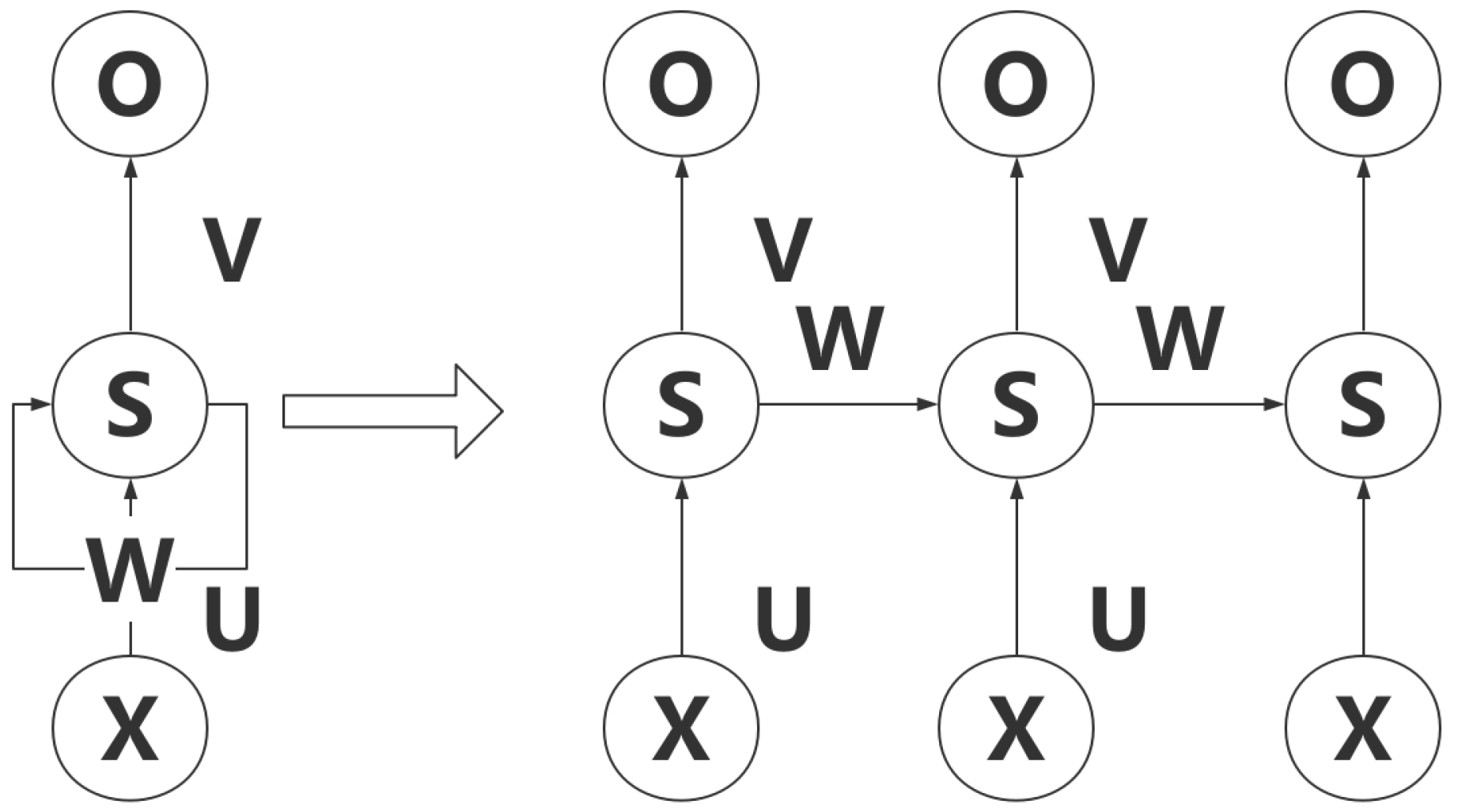
2.1. RNN
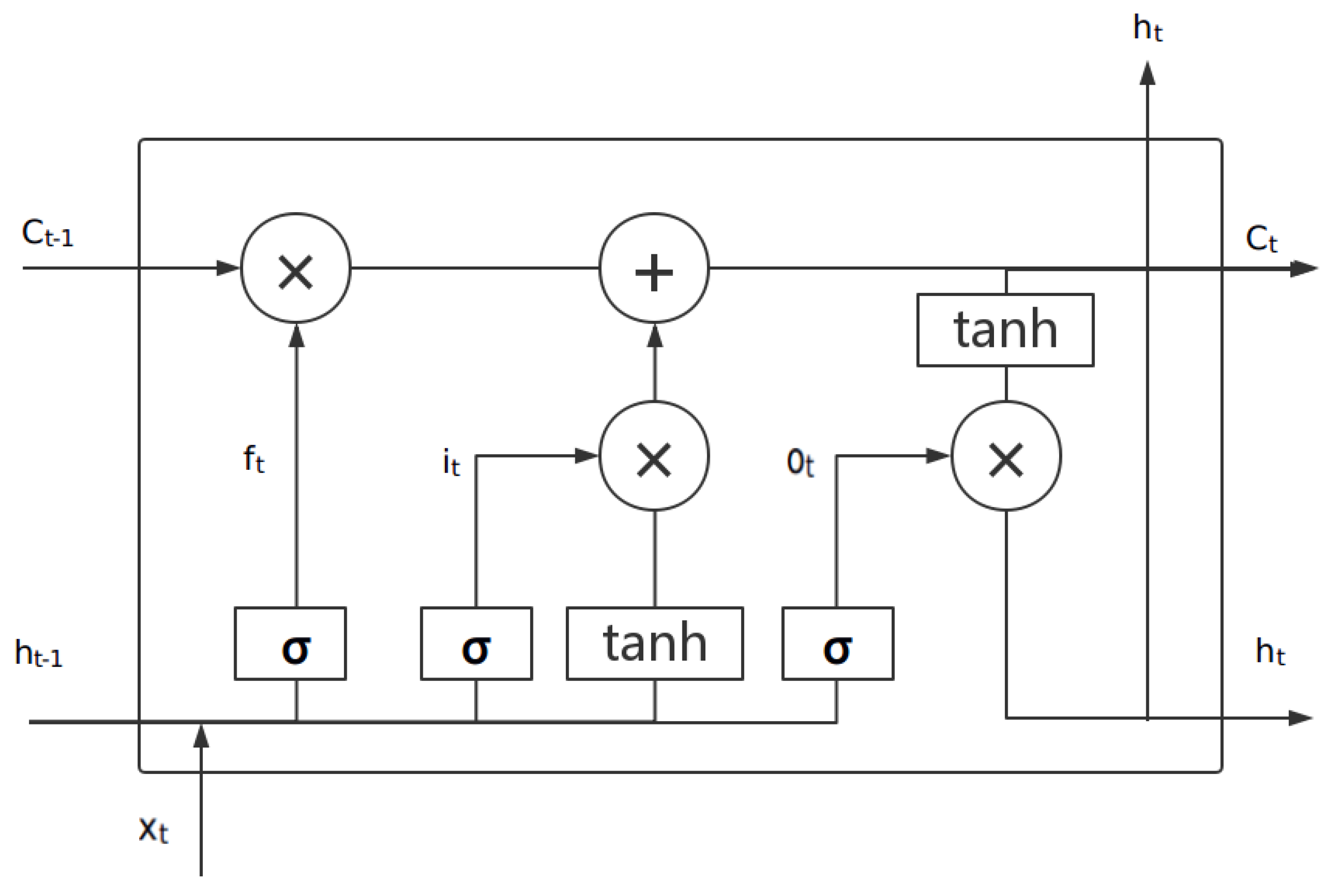
2.2. LSTM
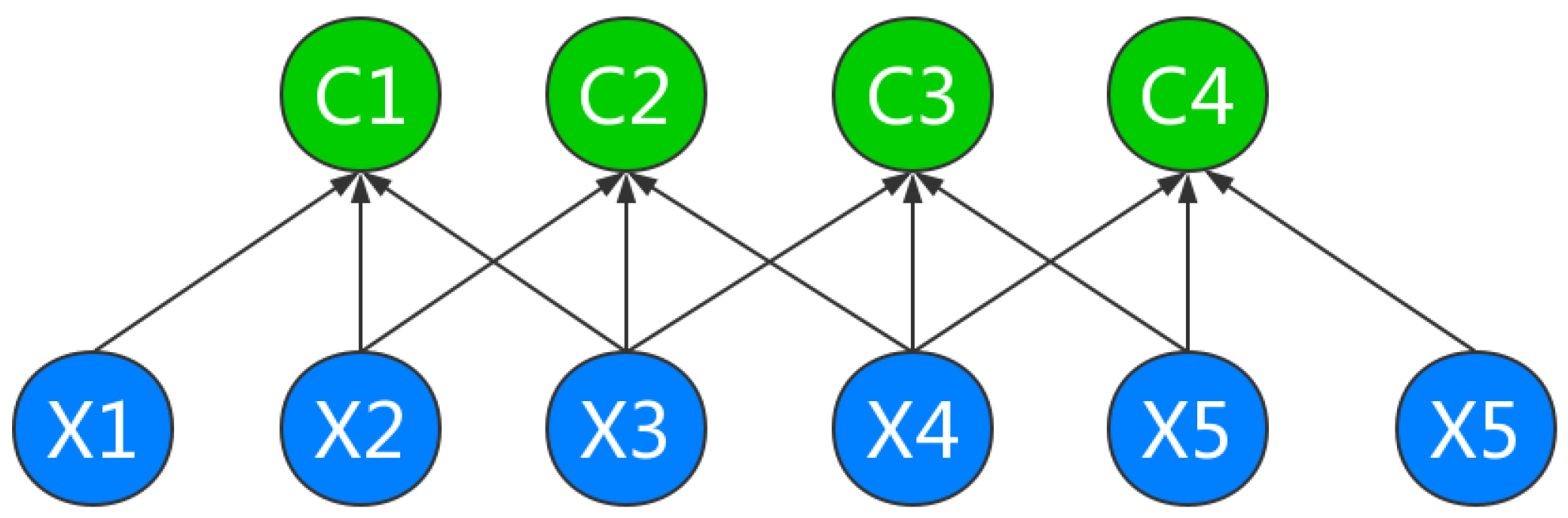
2.3. CNN
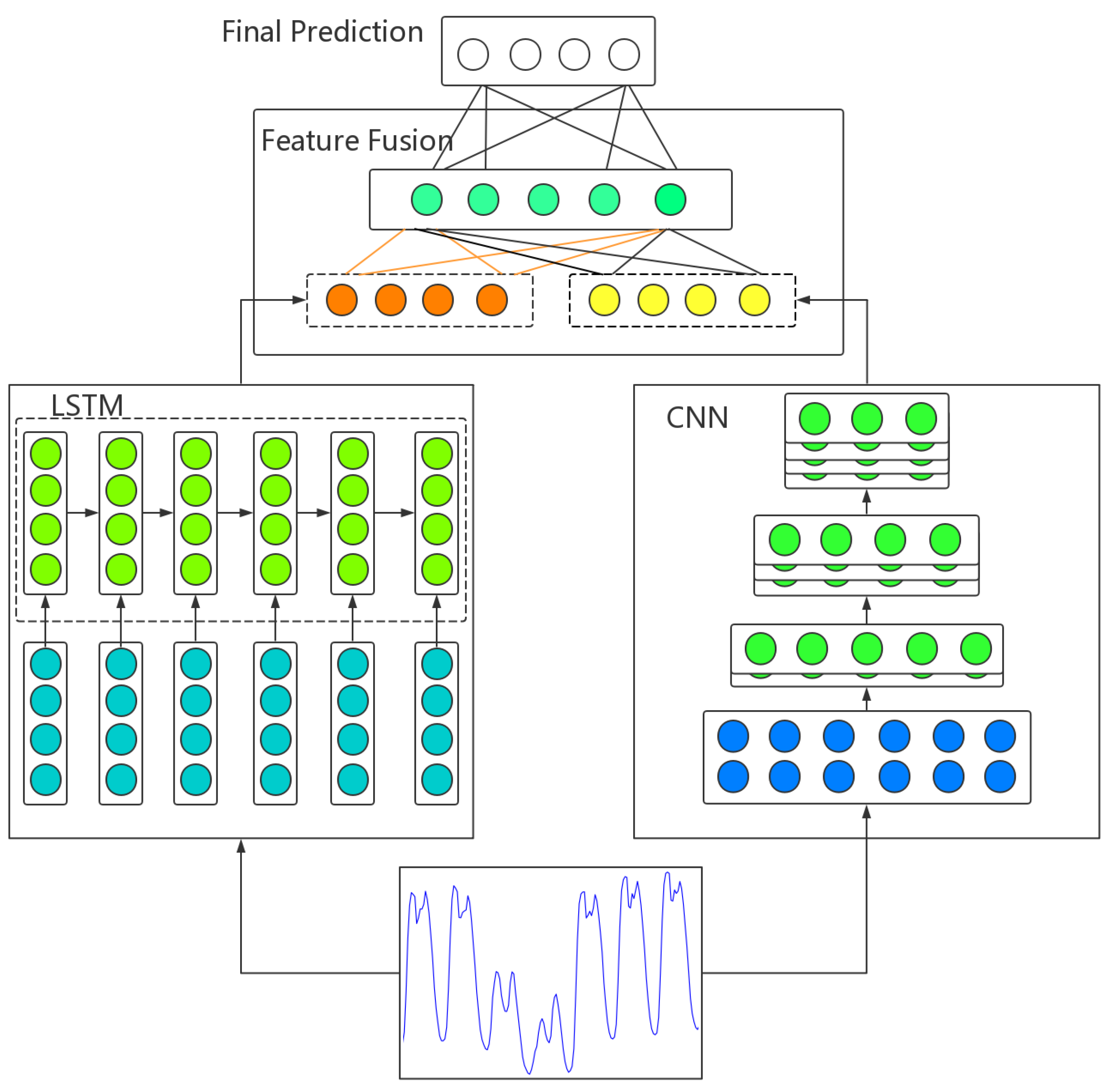
3. The Proposed Method
3.1. The Overview of the Proposed Framework
3.2. Model Evaluation Indexes
4. Experiments and Results
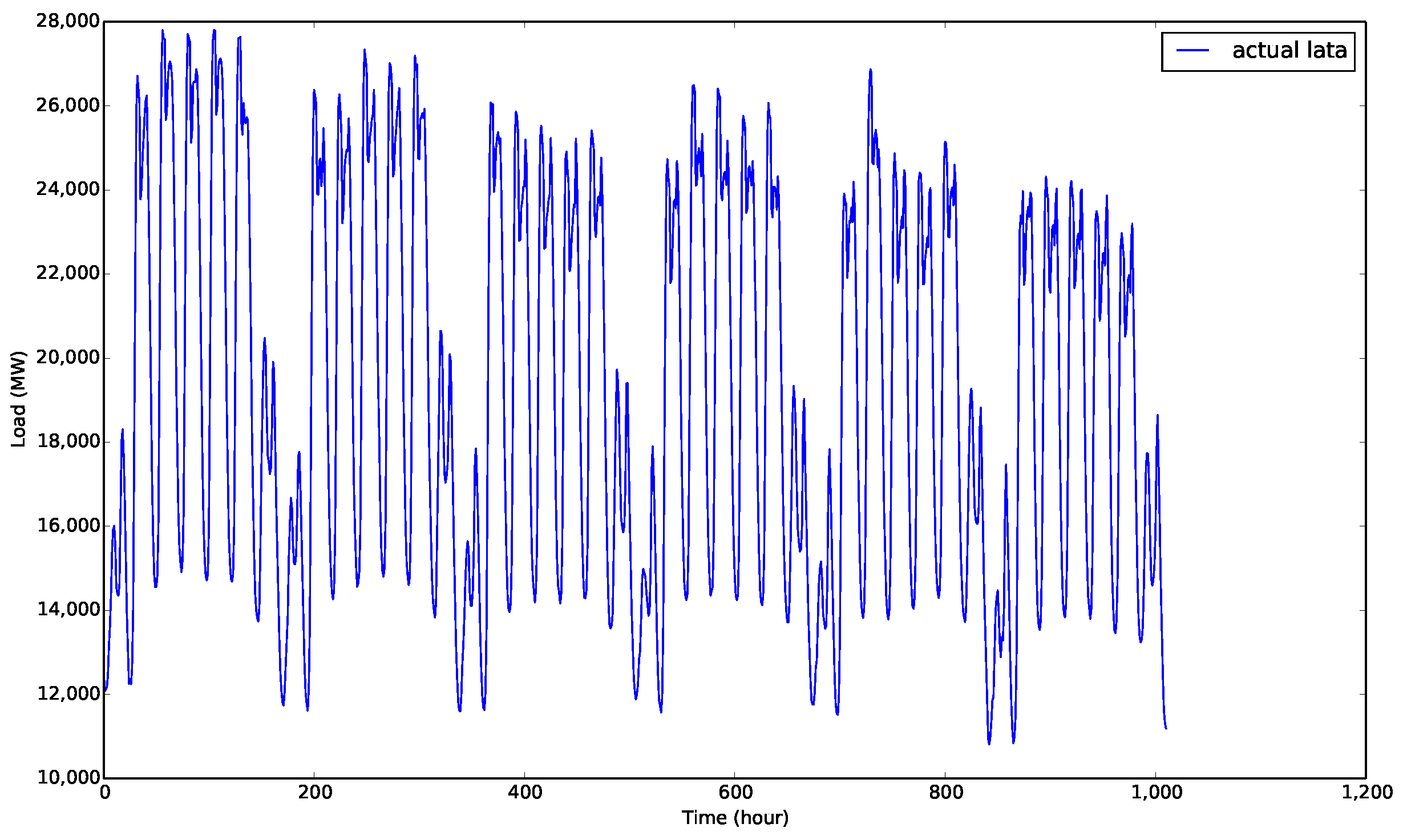
4.1. Datasets Description
4.2. The Detailed Experimental Setting
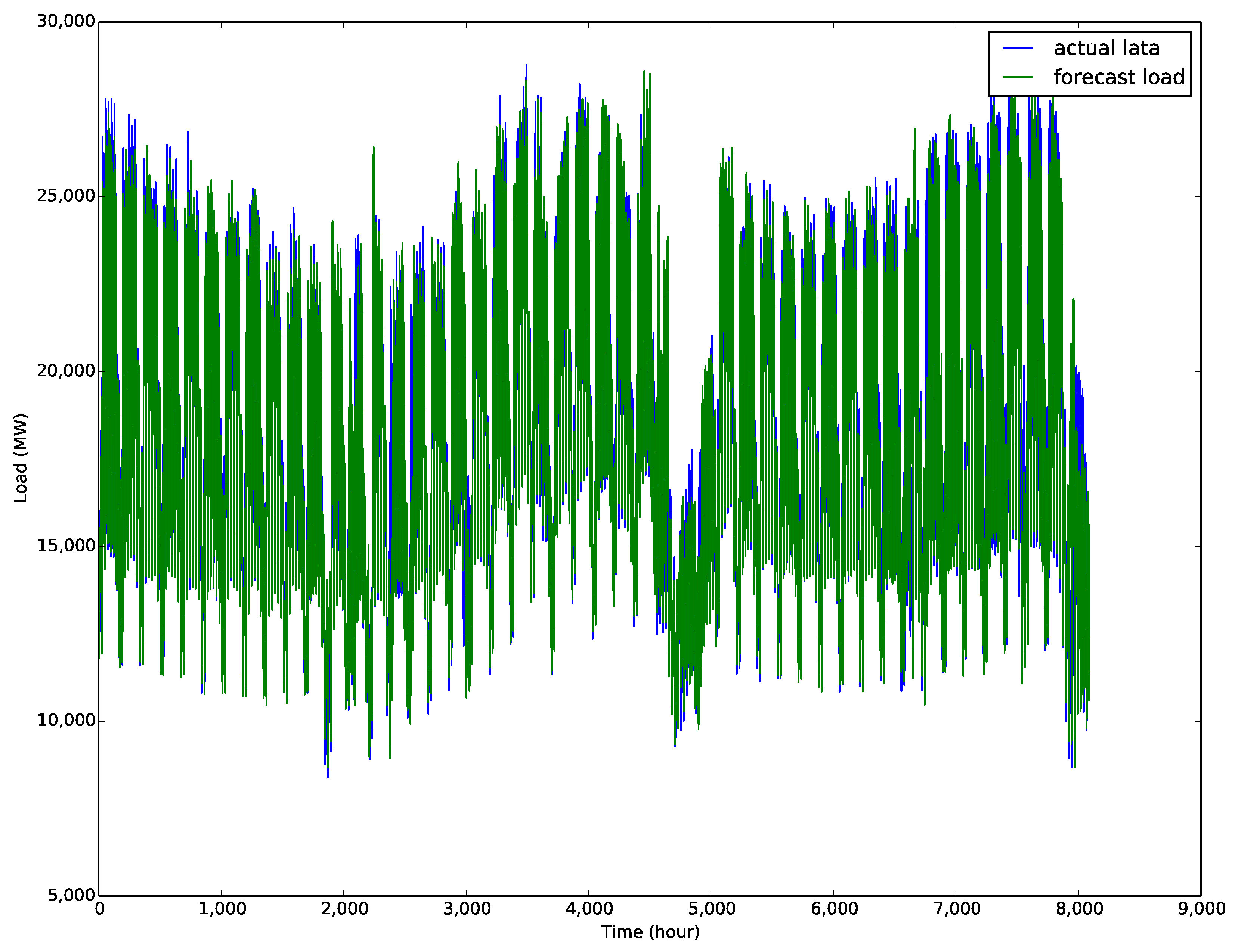
4.3. Experimental Results and Analysis
5. Discussion
6. Conclusions
Author Contributions
Funding
Conflicts of Interest
References
- Chai, B.; Chen, J.; Yang, Z.; Zhang, Y. Demand Response Management With Multiple Utility Companies: A Two-Level Game Approach. IEEE Trans. Smart Grid 2014, 5, 722–731. [Google Scholar] [CrossRef]
- Apostolopoulos, P.A.; Tsiropoulou, E.E.; Papavassiliou, S. Demand Response Management in Smart Grid Networks: A Two-Stage Game-Theoretic Learning-Based Approach. Mob. Netw. Appl. 2018, 1–14. [Google Scholar] [CrossRef]
- Chen, Y.; Luh, P.B.; Guan, C.; Zhao, Y.; Michel, L.D.; Coolbeth, M.A.; Friedland, P.B.; Rourke, S.J. Short-Term Load Forecasting: Similar Day-Based Wavelet Neural Networks. IEEE Trans. Power Syst. 2010, 25, 322–330. [Google Scholar] [CrossRef]
- Bunn, D.; Farmer, E.D. Comparative Models for Electrical Load Forecasting; Wiley: New York, NY, USA, 1986; p. 232. [Google Scholar]
- Oh, C.; Lee, T.; Kim, Y.; Park, S.; Kwon, S.B.; Suh, B. Us vs. Them: Understanding Artificial Intelligence Technophobia over the Google DeepMind Challenge Match. In Proceedings of the 2017 CHI Conference on Human Factors in Computing Systems, Denver, CO, USA, 6–11 May 2017; pp. 2523–2534. [Google Scholar]
- Skilton, M.; Hovsepian, F. Example Case Studies of Impact of Artificial Intelligence on Jobs and Productivity. In 4th Industrial Revolution; Skilton, M., Hovsepian, F., Eds.; National Academies Press: Washington, DC, USA, 2018; pp. 269–291. [Google Scholar]
- Singh, P.; Dwivedi, P. Integration of new evolutionary approach with artificial neural network for solving short term load forecast problem. Appl. Energy 2018, 217, 537–549. [Google Scholar] [CrossRef]
- Ertugrul, Ö.F. Forecasting electricity load by a novel recurrent extreme learning machines approach. Int. J. Electr. Power Energy Syst. 2016, 78, 429–435. [Google Scholar] [CrossRef]
- Zhang, Z.; Liang, G.U.O.; Dai, Y.; Dong, X.U.; Wang, P.X. A Short-Term User Load Forecasting with Missing Data. DEStech Trans. Eng. Technol. Res. 2018. [Google Scholar] [CrossRef]
- Charytoniuk, W.; Chen, M.S.; Olinda, P.V. Nonparametric regression based short-term load forecasting. IEEE Trans. Power Syst. 1998, 13, 725–730. [Google Scholar] [CrossRef]
- Song, K.B.; Baek, Y.S.; Hong, D.H.; Jang, G. Short-term load forecasting for the holidays using fuzzy linear regression method. IEEE Trans. Power Syst. 2005, 20, 96–101. [Google Scholar] [CrossRef]
- Christiaanse, W.R. Short-term load forecasting using general exponential smoothing. IEEE Trans. Power Appl. Syst. 1971, 2, 900–911. [Google Scholar] [CrossRef]
- Lee, C.M.; Ko, C.N. Short-term load forecasting using lifting scheme and ARIMA models. Expert Syst. Appl. 2011, 38, 5902–5911. [Google Scholar] [CrossRef]
- Çevik, H.H.; Çunkaş, M. Short-term load forecasting using fuzzy logic and ANFIS. Neural Comput. Appl. 2015, 26, 1355–1367. [Google Scholar] [CrossRef]
- Yu, F.; Hayashi, Y. Pattern sequence-based energy demand forecast using photovoltaic energy records. In Proceedings of the 2012 International Conference on Renewable Energy Research and Applications, Nagasaki, Japan, 11–14 November 2012; pp. 1–6. [Google Scholar]
- Barman, M.; Choudhury, N.B.D.; Sutradhar, S. Short-term load forecasting using fuzzy logic and A regional hybrid GOA-SVM model based on similar day approach for short-term load forecasting in Assam, India. Energy 2018, 145, 710–720. [Google Scholar] [CrossRef]
- Chen, Y.; Xu, P.; Chu, Y.; Li, W.; Wu, Y.; Ni, L.; Bao, Y.; Wang, K. Short-term electrical load forecasting using the Support Vector Regression (SVR) model to calculate the demand response baseline for office buildings. Appl. Energy 2017, 195, 659–670. [Google Scholar] [CrossRef]
- Ding, N.; Benoit, C.; Foggia, G.; Besanger, Y.; Wurtz, F. Neural network-based model design for short-term load forecast in distribution systems. IEEE Trans. Power Syst. 2016, 31, 72–81. [Google Scholar] [CrossRef]
- Ekonomou, L.; Christodoulou, C.A.; Mladenov, V. A short-term load forecasting method using artificial neural networks and wavelet analysis. Int. J. Power Syst. 2016, 1, 64–68. [Google Scholar]
- Merkel, G.; Povinelli, R.; Brown, R. Short-Term load forecasting of natural gas with deep neural network regression. Energies 2018, 11, 2008. [Google Scholar] [CrossRef]
- Bouktif, S.; Fiaz, A.; Ouni, A.; Serhani, M. Optimal Deep Learning LSTM Model for Electric Load Forecasting using Feature Selection and Genetic Algorithm: Comparison with Machine Learning Approaches. Energies 2018, 11, 1636. [Google Scholar] [CrossRef]
- Zheng, H.; Yuan, J.; Chen, L. Short-term load forecasting using EMD-LSTM neural networks with a Xgboost algorithm for feature importance evaluation. Energies 2017, 10, 1168. [Google Scholar] [CrossRef]
- Shi, H.; Xu, M.; Li, R. Deep Learning for Household Load Forecasting—A Novel Pooling Deep RNN. IEEE Trans. Smart Grid 2018, 9, 5271–5280. [Google Scholar] [CrossRef]
- Wei, L.Y.; Tsai, C.H.; Chung, Y.C.; Liao, K.H.; Chueh, H.E.; Lin, J.S. A Study of the Hybrid Recurrent Neural Network Model for Electricity Loads Forecasting. Int. J. Acad. Res. Account. Financ. Manag. Sci. 2017, 7, 21–29. [Google Scholar] [CrossRef]
- Gensler, A.; Henze, J.; Sick, B.; Raabe, N. Deep Learning for solar power forecasting—An approach using AutoEncoder and LSTM Neural Networks. In Proceedings of the 2016 IEEE International Conference on Systems, Man, and Cybernetics, Budapest, Hungary, 9–12 October 2016; pp. 858–865. [Google Scholar]
- Chen, Z.; Sun, L.X.; University, Z. Short-Term Electrical Load Forecasting Based on Deep Learning LSTM Networks. Electron. Technol. 2018, 47, 39–41. [Google Scholar]
- Kuan, L.; Yan, Z.; Xin, W.; Yan, C.; Xiangkun, P.; Wenxue, S.; Zhe, J.; Yong, Z.; Nan, X.; Xin, Z. Short-term electricity load forecasting method based on multilayered self-normalizing GRU network. In Proceedings of the 2017 IEEE Conference on Energy Internet and Energy System Integration, Beijing, China, 26–28 November 2018; pp. 1–5. [Google Scholar]
- Zheng, J.; Xu, C.; Zhang, Z.; Li, X. Electric load forecasting in smart grids using Long-Short-Term-Memory based Recurrent Neural Network. In Proceedings of the 51st Annual Conference on Information Sciences and Systems (CISS), Baltimore, MD, USA, 22–24 March 2017; pp. 1–6. [Google Scholar]
- Wang, Y.; Liu, M.; Bao, Z.; Zhang, S. Short-Term Load Forecasting with Multi-Source Data Using Gated Recurrent Unit Neural Networks. Energies 2018, 11, 1138. [Google Scholar] [CrossRef]
- Du, S.; Li, T.; Gong, X.; Yang, Y.; Horng, S.J. Traffic flow forecasting based on hybrid deep learning framework. In Proceedings of the 12th International Conference on Intelligent Systems and Knowledge Engineering, Nanjing, China, 24–26 November 2017; pp. 1–6. [Google Scholar]
- Kuo, P.H.; Huang, C.J. A High Precision Artificial Neural Networks Model for Short-Term Energy Load Forecasting. Energies 2018, 11, 213. [Google Scholar] [CrossRef]
- Hsu, D. Time Series Forecasting Based on Augmented Long Short-Term Memory. arXiv, 2017; arXiv:1707.00666. [Google Scholar]
- Che, Z.; Purushotham, S.; Cho, K.; Sontag, D.; Liu, Y. Recurrent Neural Networks for Multivariate Time Series with Missing Values. Sci. Rep. 2018, 8, 6085. [Google Scholar] [CrossRef]


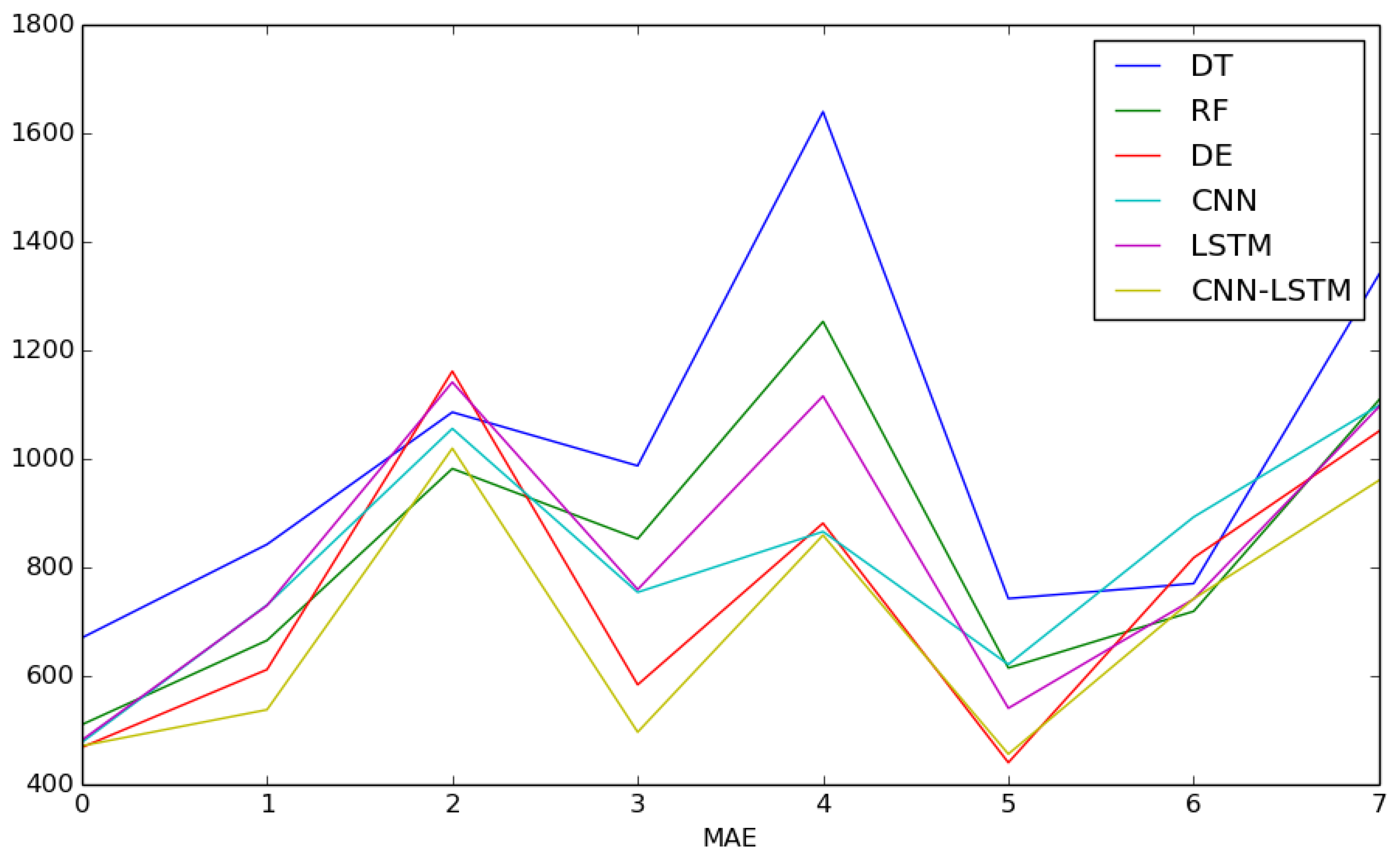
| Test | DT | RF | DE | CNN | LSTM | CNN-LSTM |
|---|---|---|---|---|---|---|
| Test-1 | 669.3277 | 509.4035 | 467.4859 | 476.7259 | 480.7812 | 470.3272 |
| Test-2 | 841.6884 | 664.7461 | 610.9937 | 730.0540 | 729.0658 | 537.0471 |
| Test-3 | 1085.2633 | 981.2681 | 1160.7618 | 1055.0703 | 1140.5746 | 1018.6435 |
| Test-4 | 986.4937 | 851.9130 | 583.1347 | 753.4446 | 758.6537 | 495.8678 |
| Test-5 | 1638.9530 | 1252.3642 | 880.7453 | 865.2113 | 1115.0330 | 858.6237 |
| Test-6 | 741.9390 | 614.0473 | 439.6090 | 620.5186 | 539.8259 | 455.3989 |
| Test-7 | 769.4685 | 718.3953 | 817.0670 | 892.1418 | 740.9322 | 741.5478 |
| Test-8 | 1339.2667 | 1107.9678 | 1050.3163 | 1097.9277 | 1095.2742 | 959.7009 |
| Test-avg | 1009.0500 | 837.5132 | 751.2642 | 811.3868 | 825.0176 | 692.1446 |
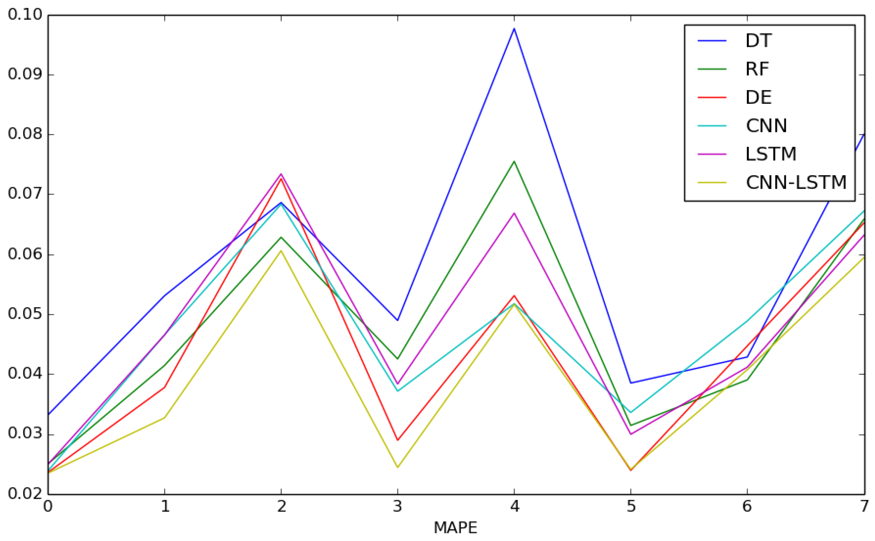
| Test | DT | RF | DE | CNN | LSTM | CNN-LSTM |
|---|---|---|---|---|---|---|
| Test-1 | 0.0332 | 0.0250 | 0.0236 | 0.0239 | 0.0249 | 0.0235 |
| Test-2 | 0.0531 | 0.0414 | 0.0378 | 0.0465 | 0.0465 | 0.0327 |
| Test-3 | 0.0686 | 0.0628 | 0.0726 | 0.0684 | 0.0734 | 0.0606 |
| Test-4 | 0.0489 | 0.0425 | 0.0289 | 0.0371 | 0.0383 | 0.0244 |
| Test-5 | 0.0977 | 0.0755 | 0.0531 | 0.0517 | 0.0669 | 0.0516 |
| Test-6 | 0.0385 | 0.0314 | 0.0239 | 0.0336 | 0.0299 | 0.0241 |
| Test-7 | 0.0428 | 0.0390 | 0.0447 | 0.0489 | 0.0411 | 0.0407 |
| Test-8 | 0.0800 | 0.0658 | 0.0652 | 0.0672 | 0.0631 | 0.0594 |
| Test-avg | 0.0578 | 0.0479 | 0.0437 | 0.0472 | 0.0480 | 0.0396 |
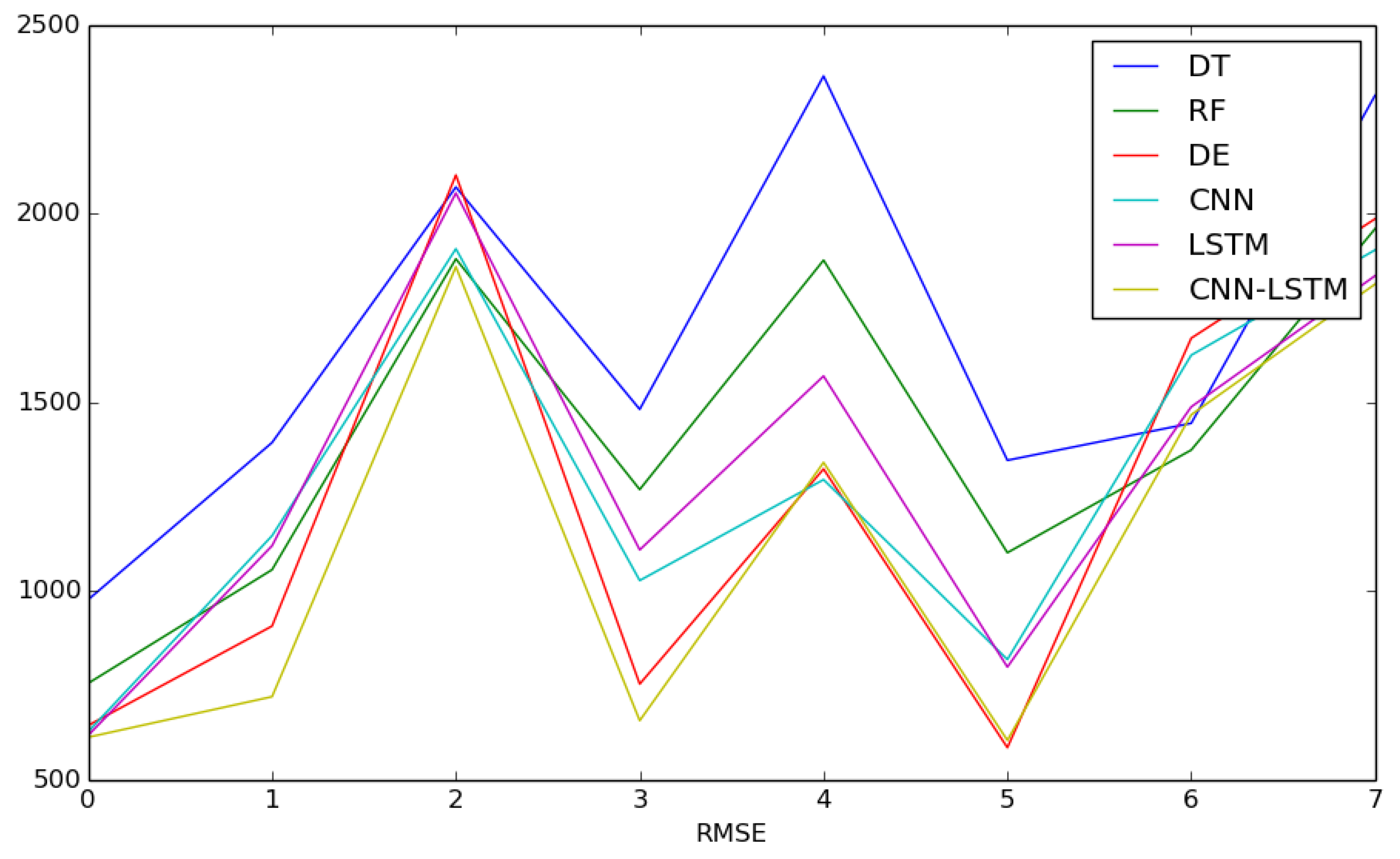
| Test | DT | RF | DE | CNN | LSTM | CNN-LSTM |
|---|---|---|---|---|---|---|
| Test-1 | 977.2206 | 755.5147 | 643.8908 | 627.4642 | 617.5835 | 612.4874 |
| Test-2 | 1393.2847 | 1056.4105 | 907.0599 | 1146.4771 | 1119.7467 | 719.9939 |
| Test-3 | 2070.3786 | 1880.0600 | 2102.2027 | 1906.8154 | 2054.4484 | 1859.0252 |
| Test-4 | 1481.5294 | 1269.0204 | 753.5586 | 1027.8778 | 1109.1206 | 656.5774 |
| Test-5 | 2364.5579 | 1876.6200 | 1323.3404 | 1295.1156 | 1569.6155 | 1340.6214 |
| Test-6 | 1346.3700 | 1101.5862 | 585.0608 | 818.5694 | 798.6015 | 604.4891 |
| Test-7 | 1444.5131 | 1373.6364 | 1669.9279 | 1624.9380 | 1487.9632 | 1467.0496 |
| Test-8 | 2313.3100 | 1959.8469 | 1986.0953 | 1903.6605 | 1835.2911 | 1813.1891 |
| Test-avg | 1673.8955 | 1409.0869 | 1246.3920 | 1293.8648 | 1324.0463 | 1134.1791 |
© 2018 by the authors. Licensee MDPI, Basel, Switzerland. This article is an open access article distributed under the terms and conditions of the Creative Commons Attribution (CC BY) license (http://creativecommons.org/licenses/by/4.0/).
Share and Cite
Tian, C.; Ma, J.; Zhang, C.; Zhan, P. A Deep Neural Network Model for Short-Term Load Forecast Based on Long Short-Term Memory Network and Convolutional Neural Network. Energies 2018, 11, 3493. https://doi.org/10.3390/en11123493
Tian C, Ma J, Zhang C, Zhan P. A Deep Neural Network Model for Short-Term Load Forecast Based on Long Short-Term Memory Network and Convolutional Neural Network. Energies. 2018; 11(12):3493. https://doi.org/10.3390/en11123493
Chicago/Turabian StyleTian, Chujie, Jian Ma, Chunhong Zhang, and Panpan Zhan. 2018. "A Deep Neural Network Model for Short-Term Load Forecast Based on Long Short-Term Memory Network and Convolutional Neural Network" Energies 11, no. 12: 3493. https://doi.org/10.3390/en11123493
APA StyleTian, C., Ma, J., Zhang, C., & Zhan, P. (2018). A Deep Neural Network Model for Short-Term Load Forecast Based on Long Short-Term Memory Network and Convolutional Neural Network. Energies, 11(12), 3493. https://doi.org/10.3390/en11123493