Solving the Multi-Objective Optimal Power Flow Problem Using the Multi-Objective Firefly Algorithm with a Constraints-Prior Pareto-Domination Approach

Abstract

Known as a multi-objective, large-scale, and complicated optimization problem, the multi-objective optimal power flow (MOOPF) problem tends to be introduced with many constraints. In this paper, compared with the frequently-used penalty function-based method (PFA), a novel constraint processing approach named the constraints-prior Pareto-domination approach (CPA) is proposed for ensuring non-violation of various inequality constraints on dependent variables by introducing the Pareto-domination principle based on the sum of constraint violations. Moreover, for solving the constrained MOOPF problem, the multi-objective firefly algorithm with CPA (MOFA-CPA) is proposed and some optimization strategies, such as the crowding distance calculation and non-dominated sorting based on the presented CPA, are utilized to sustain well-distributed Pareto front (PF). Finally, in order to demonstrate the feasible and effective improvement of MOFA-CPA, a comparison study between MOFA-CPA and MOFA-PFA is performed on two test systems, including three bi-objective optimization cases and three tri-objective optimization cases. The simulation results demonstrate the capability of the MOFA-CPA for obtaining PF with good distribution and superiority of the proposed CPA for dealing with inequality constraints on dependent variables. In addition, some quality indicators are used to evaluate the convergence, distribution, and uniformity of the PFs found by the MOFA-CPA and MOFA-PFA.

1. Introduction

Most engineering and scientific optimization problems in the real world involve multiple objective functions with different meanings and non-commensurable units, making it difficult to simultaneously optimize multiple objectives [1,2]. The fundamental task of the power industry is to ensure safe and reliable power generation and supply under the conditions of sufficient and reasonable utilization of operating equipment in order to meet electricity demands [3]. For such an important energy conversion system as the electric power grid, reducing fuel consumption and increasing operational efficiency with sufficient power supply will lead to significant fuel savings each year [4,5]. In the early 1960s, French scholar Carpentier proposed the optimal power flow (OPF) model for the first time on the basis of precise mathematics and set a milestone in the theory of optimal operation of power systems [6]. The OPF problem achieves an optimal objective function of the power grid by means of regulating generators’ active power outputs, voltage amplitudes, transformers’ tap selection, and reactive power compensators’ reactive power switching to adjust the power flow and ensure dependent variables’ values within specified limits in order to achieve secure, efficient, and economical operation of the power grid [7,8]. Multi-objective optimal power flow (MOOPF) has become an indispensable application in power systems due to the increasing objectives needing to be optimized [9,10,11].

Multi-objective evolutionary algorithms (MOEAs), multi-objective swarm optimization algorithms, and multi-objective meta-heuristic algorithms have been suggested and utilized to solve multi-objective problems (MOPs) effectively [12]. For example, in [13], the authors proposed a modified MOEA/D algorithm with repair strategy and penalty function for constraints processing to solve the MOOPF problem. A tri-objective differential evolution (DE) approach was carried out for the TOP problem contains all global optima of the MMOP in [14]. In [15], Emilio Barocio implemented the modified flower pollination algorithm (MFPA) to calculate the PFs under different objective combinations of the MOOPF problem, using added penalty functions to handle the constraints. The authors used the non-dominated sorting multi-objective gravitational search algorithm (NSMOGSA) to solve the MOOPF problem, its applicability to large systems remains to be tested due to the effectiveness of the proposed algorithm is only tested on a standard IEEE 30-bus power system [16]. Mostafa Sedighizadeh used the Hybrid Big Bang Big Crunch (HBB–BC) algorithm to tackle the multi-objective reconfiguration and capacitor placement in fuzzy framework [17]. In addition, Al-Attar proposed a novel moth swarm algorithm (MSA) which uses the influence of moonlight on the moth direction to solve the constrained MOOPF problem in [18]. In [19], the authors presented the application of a new effective meta-heuristic optimization method, namely, non-dominated cuckoo search algorithm (NSCS) to deal with MOPs in a wind thermal power system. Although the above-mentioned methods show good performance in solving MOPs, it is still difficult to apply these methods to solve constrained MOOPF problems when it comes to a large system like IEEE 57-bus system [20]. Thus, it is necessary to propose alternative methods to effectively deal with constraints on the dependent variables of MOOPF problems.

With regard to the constrained MOOPF problem, inequality constraints can be classified into inequality constraints on independent variables and on dependent variables. Independent variables can be limited within the allowable range when the algorithm is initialized [21]. The dependent variables are computed based on the given independent variables, and it is difficult to determine whether they are satisfied [22]. Effective methods must be adopted to deal with it. Most of the reported algorithms used a penalty function approach (PFA) to deal with constraints on dependent variables, but the PFA does not fully guarantee the variables within limits [23]. In recognition of the disadvantages in those previously proposed methods, we propose a multi-objective firefly algorithm with a novel constraint processing approach (MOFA-CPA) to solve the constrained MOOPF problem. The constraints-prior Pareto-domination method (CPA) is proposed for guiding the population to the feasible region and ensuring none violation of various inequality constraints on dependent variables. With the intention of sustaining a well-distributed Pareto front (PF), crowding distance and non-dominated sorting based on the presented CPA are adopted. In order to demonstrate the feasible and effective improvement of CPA, a comparison study between MOFA-CPA and MOFA-PFA is performed on the IEEE 30-bus and IEEE 57-bus systems including three bi-objective optimization cases and three tri-objective optimization cases. The simulation results demonstrate the capability and superiority of the MOFA-CPA for obtaining PF with good distribution and processing constraints. In addition, some quality indicators are considered to evaluate the convergence, distribution, and diversity of the PFs found by MOFA-CPA and MOFA-PFA.

The remainder of the paper is organized as follows. Section 1 describes some concepts of MOPs. Section 2 introduces the mathematical formulation of MOOPF problem. Section 3 proposes a MOFA algorithm based on CPA and PFA methods. Section 4 presents simulation results and analysis. Finally, the conclusion is made in Section 5.

2. Mathematical Modeling of the MOOPF Problem

In mathematics, maximization and minimization problems are essentially the same and can be transformed into each other [24]. Therefore, the MOOPF problem can be defined as an optimization problem that includes the following n decision variables, m objective functions, and several constraints. The mathematical model is expressed as follows.

$$\begin{array}{c}\min f=(f_1(s,c),f_2(s,c),\cdots f_m(s,c))\\ s.t.g_p(s,c)\ge 0,p=1,2,\cdots ,P\\ h_q(s,c)=0,q=1,2,\cdots ,Q\end{array}$$

(1)

In the Equation (1), c = (c₁, c₂, …, c_n) is a vector of decision variables, s is a vector of dependent variables, g_p(s,c) are inequality constraints, h_q(s,c) are equality constraints, and P and Q mean the number of inequality constraints and equality constraints, respectively.

2.1. Objective Functions

The objective functions are formulated to minimize the quadratic fuel cost function, fuel cost with value-point loadings, real power losses of transmission, and fuel cost emission.

The quadratic fuel cost function in terms of real power output is shown in Equation (2).

$$f_{\mathrm{cost}}={\displaystyle \sum _{i=1}^{N_g}(a_i+b_i{P}_{gi}+c_i}{P}_{gi}^2)\$/h$$

(2)

where f_cost is the total basic fuel cost, its unit is $/h, N_g is the total number of generators, a_i, b_i, and c_i are the fuel cost coefficients of the bus i, P_gi is the real power of the ith generator.

The second objective function can be stated as the following formula.

$$f_{\cos \mathrm{t}\_\mathrm{vp}}={\displaystyle \sum _{i=1}^{N_g}(a_i+b_i{P}_{gi}+c_i}{P}_{gi}^2+\left|d_i\times \sin (e_i\times (P_{gi}^{\min }-P_{gi}))\right|)\$/h$$

(3)

where f_{cost_vp} is the total fuel cost with valve-point effect, its unit is $/h, d_i and e_i are cost coefficients of the bus i with valve-point effect, P_gi^min is the lower real power of bus i.

The third objective function is shown as follows.

$$f_{Ploss}={\displaystyle \sum _{l=1}^{N_l}{C}_l[V_i^2+V_j^2-2V_i{V}_j\cos {\delta }_{ij}]}\mathrm{MW}$$

(4)

where f_Ploss denotes total active power losses, its unit is MW, N_l is the total number of branches in the power system, C_l is the conductance of branch l, bus i and bus j are the two terminals of branch l, V_i and V_j are the voltage magnitude of bus i and bus j, respectively. δ_ij is the voltage angle difference between bus i and bus j.

Total emission caused by SO_x and NO_x can be stated as the following equation.

$$f_{emission}={\displaystyle \sum _{i=1}^{N_g}[{\alpha }_i{P}_{gi}^2+{\beta }_i{P}_{gi}+{\gamma }_i}+{\eta }_i\exp ({\lambda }_i{P}_{gi})]\mathrm{ton}/\mathrm{h}$$

(5)

where f_emission is the fourth minimization, its unit is ton/h, α_i, β_i, γ_i, η_i, and λ_i are the emission coefficients of generator i.

2.2. Equality Constraints

Using Newton’s method to solve the power flow, the node’s active power balance equation is given in Equation (6).

$$P_{Gi}-P_{Di}-V_i{\displaystyle \sum _{j\in N_i}^{}{V}_j(G_{ij}\cos {\delta }_{ij}+B_{ij}\sin {\delta }_{ij})=0}\begin{array}{cc}& i\in N\end{array}$$

(6)

The reactive power balance equation for each PQ node is shown in Equation (7).

$$Q_{Gi}-Q_{Di}-V_i{\displaystyle \sum _{j\in N_i}^{}{V}_j(G_{ij}\sin {\delta }_{ij}-B_{ij}\cos {\delta }_{ij})}=0\begin{array}{cc}& i\in N_{pq}\end{array}$$

(7)

The equality constraints are consisted of Equations (6) and (7). The specific meaning of each element can be taken from the literature [25].

2.3. Inequality Constraints

The inequality constraints on independent variables can be represented by Equations (8)–(12). The specific meaning of each element can be taken from the literature [25].

$$c^T=\left[P_{g2},\cdots ,P_{g{N}_g},V_{g1},\cdots ,V_{g{N}_g},T_1,\cdots ,T_{N_t},Q_{c1},\cdots ,Q_{c{N}_c}\right]$$

(8)

• Limits of P_g

  $$P_{gi,\min }\le P_{gi}\le P_{gi,\max },i\in N_g\cap i\notin \mathrm{ref}$$

  (9)
• Limits of V_g

  $$V_{gi,\min }\le V_{gi}\le V_{gi,\max },i\in N_g$$

  (10)
• Limits of T

  $$T_{i,\min }\le T_i\le T_{i,\max },i\in N_t$$

  (11)
• Limits of Q_c

  $$Q_{ci,\min }\le Q_{ci}\le Q_{ci,\max },i\in N_c$$

  (12)

The inequality constraints on dependent variables can be represented by Equations (13)–(17). The specific meaning of each element can be found in the literature [25].

$$s^T=\left[P_{g\mathrm{ref}},V_{l1},\cdots ,V_{l{N}_{pq}},Q_{g1},\cdots ,Q_{g{N}_g},S_1,\cdots ,S_{N_l}\right]$$

(13)

• Limits of P_gref

  $$P_{g\mathrm{ref},\min }\le P_{g\mathrm{ref}}\le P_{g\mathrm{ref},\max }$$

  (14)
• Limits of V_l

  $$\begin{array}{c}{V}_{li,\min }-V_{li}\le 0\\ V_{li}-V_{li,\max }\le 0\end{array},i\in N_{pq}$$

  (15)
• Limits of Q_g

  $$\begin{array}{c}{Q}_{gi,\min }-Q_{gi}\le 0\\ Q_{gi}-Q_{gi,\max }\le 0\end{array},i\in N_g$$

  (16)
• Limits of S

  $$S_{ij}-S_{ij,\max }\le 0,ij\in N_l$$

  (17)

2.4. Constraints Processing

When we use intelligent algorithms to solve MOOPF problems, the major difficulty is how to effectively deal with the constraints described in Section 2.2 and Section 2.3.

The equality constraints are able to be limited in allowable boundaries in the process of running Newton–Raphson load flow calculation, and the independent variable on independent variables can be repaired as follows when it violates its own specified range.

$$c_i=\{\begin{array}{l}{c}_{i\min }if{c}_i<c_{i\min }\\ c_{i}if{c}_{i\min }<c_i<c_{i\max }\\ c_{i\max }if{c}_i>c_{i\max }\end{array}$$

(18)

2.4.1. Penalty Function Approach

For the inequality constraints on dependent variables, the most common method for processing constraints in many intelligent algorithms is the usage of PFA. The PFA converts the constrained MOOPF problem into an unconstrained one, as shown in Equations (19) and (20).

$$\min f_{i\_pf}=\min (f_i+penalty)$$

(19)

$$\begin{array}{ll}\hfill penalty& =K_V{\displaystyle \sum _{i=1}^{N_{pq}}(V_{li}-V_{Li}^{\lim })}+K_Q{\displaystyle \sum _{i=1}^{N_g}(Q_{gi}-Q_{gi}^{\lim })}\hfill \\ & +K_S(P_{g\mathrm{ref}}-P_{g\mathrm{ref}}^{\lim })+K_L{\displaystyle \sum _{i=1}^{N_l}(S_i-S_i^{\lim })}\hfill \end{array}$$

(20)

where f_i is the ith objective function, K_V, K_Q, K_S, K_L are penalty factors, lim means the boundary value of their own specified range.

2.4.2. Proposed Constraints-Prior Pareto-Domination Approach

When using the PFA illustrated in Section 2.4.1, the constraint violations are used to punish an infeasible solution so that feasible solutions are chosen by the selection procedure. Despite the widespread application of PFA, it has several disadvantages, among which the salient one is that it involves frequent correction for the penalty coefficients. In order to overcome the shortcoming of PFA, the constraints-prior Pareto-domination approach (CPA) is proposed in this paper for processing inequality constraints on dependent variables, which is totally different from the PFA algorithm. Since no penalty coefficient is needed, the inconvenience of frequent correction for the penalty coefficients can be avoided with the aim of improving the efficiency of solving the MOOPF problem. Also, it does not need any supplementary parameters, unlike PFA.

With regard to inequality constraints on dependent variables, the steps of our suggested CPA to deal with them are expressed as follows.

At the start, the sum of constraint violations will be calculated by the following formula when independent variable c_i violates its own specified range.

$$Svio(c_i)={\displaystyle \sum _{j\in u}\max (g_p(s,c_i)},0)u\in P$$

(21)

where u is the number of particular inequality constraints on dependent variables.

Secondly, randomly select two different solutions known as a set of independent variables c₁ and c₂, and then determine the sum of constraint violations of c₁ and c₂.

Before the categorizing process, we will first introduce the Pareto dominance method. When both conditions in the Equation (22) are satisfied, c₁ Pareto dominates c₂.

$$\{\begin{array}{c}\forall i\in \{1,2,\dots ,m\}:f_i(s,c_1)\le f_i(s,c_2)\\ \exists j\in \{1,2,\dots ,m\}:f_j(s,c_1)<f_j(s,c_2)\end{array}\Rightarrow c_1\prec c_2$$

(22)

This relationship shows that there are two possibilities for any two decision variables, one of which takes the other decision variable or each other does not be dominated.

And then, the categorizing process to determine the dominated relationship is as follows.

If Svio (c₁) = Svio (c₂), and only if the two equations shown in the Equation (22) are satisfied simultaneously, c₂ will be dominated by c₁, which marks as c₁ $\prec$ c₂.

If Svio (c₁) < Svio (c₂), it can be inferred that c₁ will dominate c₂, which marks as c₁ $\prec$ c₂.

If Svio (c₁) > Svio (c₂), it indicates that c₁ will be dominated by c₂, which marks as c₂ $\prec$ c₁.

Finally, if c₁ $\prec$ c₂, c₁ will be chosen as a Pareto optimal solution. If c₂ $\prec$ c₁, c₂ will be chosen as a Pareto optimal solution, the surface defined by the objective vector corresponding to the Pareto optimal solution is called the Pareto front (PF).

The proposed CPA algorithm not only can be used to deal with constraints on dependent variables, but also can be used to reconstruct the concept of Pareto-dominant in the non-dominate sorting.

3. MOFA Algorithm

3.1. Basic Firefly Algorithm

In 2010, Zhao et al. proposed FA to solve optimized problem illuminated by the relationship of firefly population (FP) [26,27,28]. The initial population of N_F fireflies is initialized based on Equation (23).

$$c_{i,d}=c_{d,\min }+rand\cdot \left(c_{d,\max }-c_{d,\min }\right)i\in \left[1,N_F\right],d\in \left[1,D\right]$$

(23)

The position vector c_i = (c_i1, c_i2, …, c_iD) of the firefly i, which is considered as a Pareto optimal solution of the MOOPF problem.

The update strategy of FA is shown in the Equation (24).

$$c_i^{new}=c_i^{old}+{\beta }_0\exp (-\gamma r_{ij}^2)(c_j^{old}-c_i^{old})+\alpha \ast {\xi }_i$$

(24)

where γ is the light absorption coefficient, β₀ is the attractiveness at r_ij = 0, α is the randomization parameter and ξ_i is a vector of random numbers with Gaussian or uniform distributions.

The distance r_ij can be calculated by Equation (25).

$$r_{ij}=\Vert c_i-c_j\Vert =\sqrt{{\displaystyle \sum _{k=1}^D{(c_{i,k}-c_{j,k})}^2}}$$

(25)

where c_i,k is the kth dimension of independent variable c_i of the firefly i, c_j,k is the kth component of the independent variable c_j of the firefly j.

Unlike the basic FA, for MOFA-PFA and MOFA-CPA algorithms, the movement of fireflies is subject to the non-dominated solution, but not a single objective solution. Section 3.2 and Section 3.3 will describe the MOFA-PFA and MOFA-CPA algorithms.

3.2. MOFA-PFA Algorithm

By extending the basic ideas of FA and combining some concepts of MOPs, the fast non-dominated sorting method and the crowding distance calculation [20] are utilized to generate PF. It is worth mentioning that the MOFA-PFA algorithm is such a MOFA algorithm that uses the commonly-used PFA to handle constraints, which is described as the pseudo code listed in

Table 1. Pseudo code of the multi-objective firefly algorithm–penalty function algorithm (MOFA-PFA).

1  population initialization;

2  while t ≤ maximum iteration Tmax

3     read the algorithm parameters;

4      set penalty factors KV, KQ, KS, KL;

5      calculate the value of the objective functions as Section 2.1 shown;

6      calculate the penalty according to the Equation (20), and added to the objective functions;

7      for i = 1 to NF do

8            for j = 1 to NF do

9                if cjold Pareto-dominates ciold according to Equation (22)

10                   generate new solution cinew as Equation (24) shown;

11                   if cinew Pareto-dominates ciold

12                       select cinew as the new solution in the FP;

13           end

14           else

15                       select ciold as the new solution in the FP;

16          end

17          end

18        end

19      end

20      update and output the Pareto optimal solutions to next iterations;

21      sort and find the current best approximation to the Pareto front;

22      t++;

23    end

.

3.3. MOFA-CPA Algorithm

Suggested MOFA-CPA is such a MOFA algorithm that has the proposed CPA method. Unlike fast non-dominated sorting methods used in MOFA-PFA, the improved fast non-dominated sorting strategy is based on the proposed CPA.

Table 2. Pseudo code of the multi-objective firefly algorithm–constraints-prior Pareto-domination approach (MOFA-CPA) algorithm.

1    population initialization;

2    while t ≤ maximum iteration Tmax

3      read the algorithm parameters;

4      calculate the value of the objective functions as Section 2.1 shown;

5      for i = 1 to NF do

6        for j = 1 to NF do

7          if cjold constraints-prior Pareto-dominates ciold using proposed CPA in Section 2.4.2;

8            generate new solution cinew as Equation (24) shown;

9           if cinew constraints-prior Pareto-dominates ciold

10               select cinew as the new solution in the FP;

11          end

12          else

13               select ciold as the new solution in the FP;

14          end

15         end

16        end

17      end

18      update and output the Pareto optimal solutions to next iterations;

19      sort and find the current best approximation to the Pareto front;

20      t++;

21    end

describes the pseudo code of MOFA-CPA, which provides an illustration of the difference between MOFA-CPA and MOFA-PFA.

3.4. Stopping Condition

Different from a single-objective optimization problem, the multiple conflict objective functions in the MOOPF problem will produce an approximate PF instead of a single solution. The purpose of designing a multi-objective optimization algorithm is to find this approximate PF. In general, there are two types of stopping condition for the MOFA algorithm, one of which meets when the generation equals the number of maximum iterations, another of which is when the MOFA algorithm finds the real PF in advance. The MOFA algorithm shows a preference for the first one due to the uncertainty of the real PF.

4. Simulation Results and Analysis

The IEEE 30-bus test system and IEEE 57-bus test system have been used to exemplify the proposed MOFA-CPA in comparison with MOFA-PFA. The detailed data of the IEEE 30-bus test system is provided in [7,29]. The detailed data of the IEEE 57-bus test system is provided in [18]. The adjusted real power upper limit of generator 9 is 85 MVAr. It is worth making clear that the steps of dependent variables T and Q_C in two test systems are both 0.001.

The software was developed in MATLAB 2012a platform and ran in a Microsoft Windows 7 PC with Intel(R) Core(TM) i5-2430M CPU @ 2.40 GHz with 4 GB Random Access Memory (RAM). Before choosing objective combinations, it is necessary to figure out the conflicting relationship among the four objective functions described in Section 2.1, as illustrated in the literature [25]. Thus, the details of the six cases are listed in

Table 3. Different objective combinations of MOFA-CPA and MOFA-PFA.

Test Cases	Objective Combinations	Test System
Case 1	min f1 = fcost&f2 = fPloss	IEEE 30
Case 2	min f1 = fcost_vp&f2 = fPloss
Case 3	min f1 = fcost_vp&f2 = femission
Case 4	min f1 = fcost&f2 = fPloss&f3 = femission
Case 5	min f1 = fcost_vp&f2 = fPloss&f3 = femission
Case 6	min f1 = fcost&f2 = fPloss&f3 = femission	IEEE 57

.

4.1. Algorithm Parameters

In order to find the most suitable algorithm parameters, the algorithm parameters are tuned many times. Then, the tuned algorithm parameters of the MOFA-CPA and MOFA-PFA are shown in

Table 4. Algorithm parameters of MOFA-CPA and MOFA-PFA for Cases 1–6.

Parameters	Case 1	Case 2	Case 3	Case 4	Case 5	Case 6
FP Size	100	100	100	100	100	100
Tmax	300	300	300	500	500	500
γ	1	1	1	1	1	1
α	0.1	0.1	0.1	0.1	0.1	0.1
β0	1	1	1	1	1	1
Trials	30	30	30	30	30	30

. For the bi-objective cases, the T_max is chosen 300 to reduce the computational complexity. For tri-objective cases and lager test systems, the maximum iteration is chosen as 500. To ensure consistency, the algorithm needs to run in 30 trials, and some steps of solving the MOOPF problem by MOFA-CPA algorithms are presented in the flowchart shown in Figure A1.

4.2. PF Computation of IEEE30

In this section, Cases 1–5, including three bi-objective optimizations and two tri-objective optimizations, are performed. The five cases analyzed in this section vary in the distribution of the PF, approximation between the obtained PF and true PF, and the ability to move towards a wider area.

To verify the effectiveness and performance of the proposed MOFA-CPA algorithm, the PFs of the optimization study Case 1 obtained by MOFA-CPA and the compared MOFA-PFA are shown in Figure 1. It appears that the PF obtained with cost and loss minimization by MOFA-CPA is well distributed over the PF obtained with cost and loss minimization by MOFA-PFA. It can also be observed that the PF of MOFA-CPA is closer to true PF than the PF of MOFA-PFA.

The proposed MOFA-CPA technique and compared MOFA-PFA algorithm have been used for Case 2 and the obtained PFs are given in Figure 2. One conclusion that can be made from this figure is that cost with value point effect makes it more difficult to solve this case and increases the computation time. Furthermore, the evaluation of both objective functions shows that all the true Pareto optimal solutions cannot be obtained by both algorithms, some of the solutions of MOFA-PFA are inferior, and MOFA-CPA method finds more Pareto optimal solution close to the true Pareto optimal solutions.

Figure 3 shows the PFs of emission and loss with value point effect minimization obtained by MOFA-CPA and MOFA-PFA. From this figure, it can be seen that MOFA-CPA has the ability to cross over inferior solutions obtained by MOFA-PFA and get better Pareto optimal solutions with a better approximation.

To verify the effectiveness of the proposed constraints processing approach, in Case 4 and Case 5, the basic cost and cost with value point effect have been considered as tri-objective simultaneous minimization with loss and emission objectives, respectively. Figure 4 and Figure 5 show the optimal PFs of MOFA-CPA and MOFA-PFA for the tri-objective minimization cases.

Beyond expectation, a more regular PF shown in Figure 5 is obtained despite non-linearity effects generated by valve-point effects. It is clearly observed from the figures that MOFA-CPA obtains better distributed and approximated PFs compared with MOFA-PFA for the two cases. It is also found that both MOFA-CPA and MOFA-PFA have the ability for solving tri-objective simultaneous minimization while MOFA-CPA has a stronger constraints processing capability.

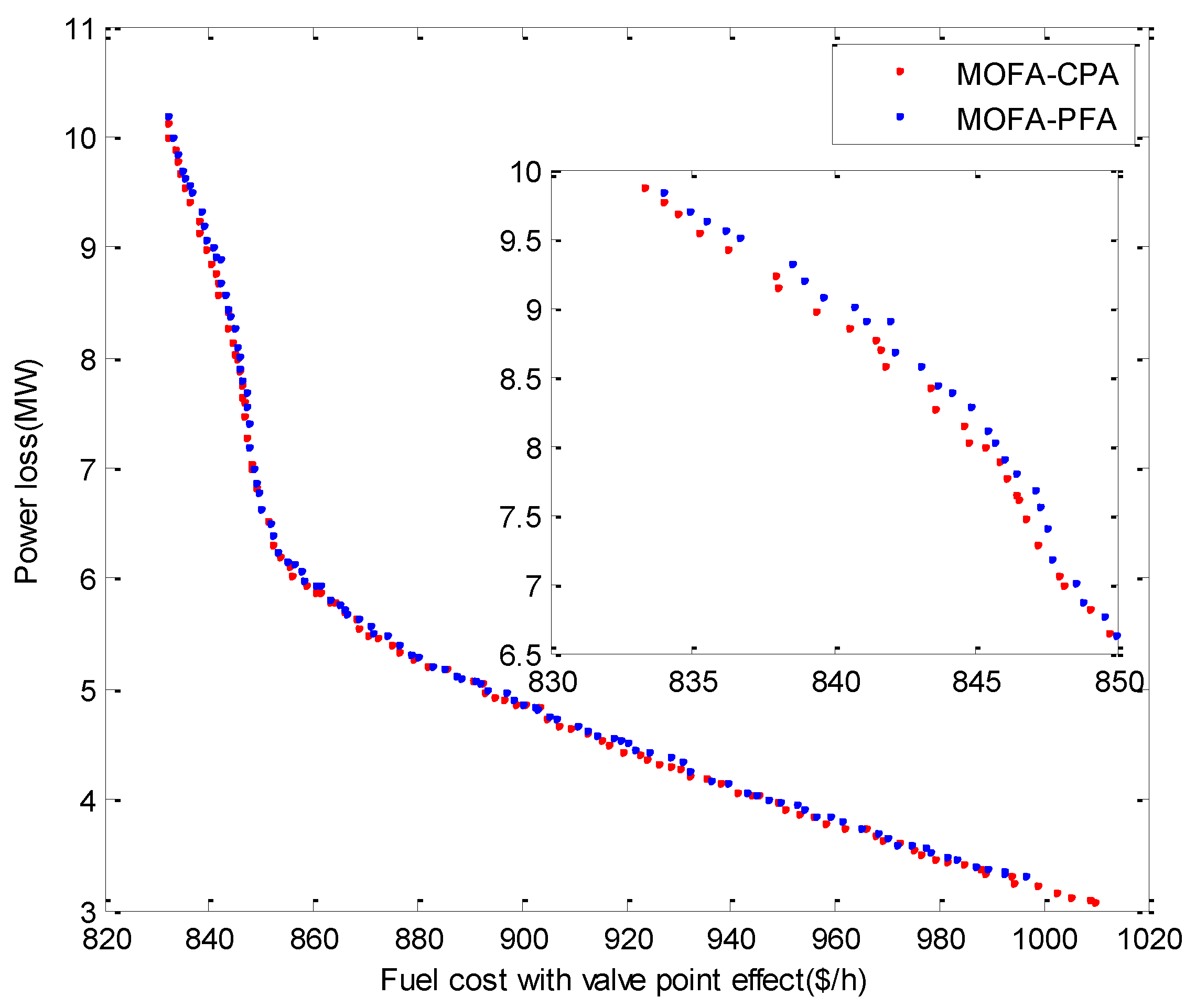
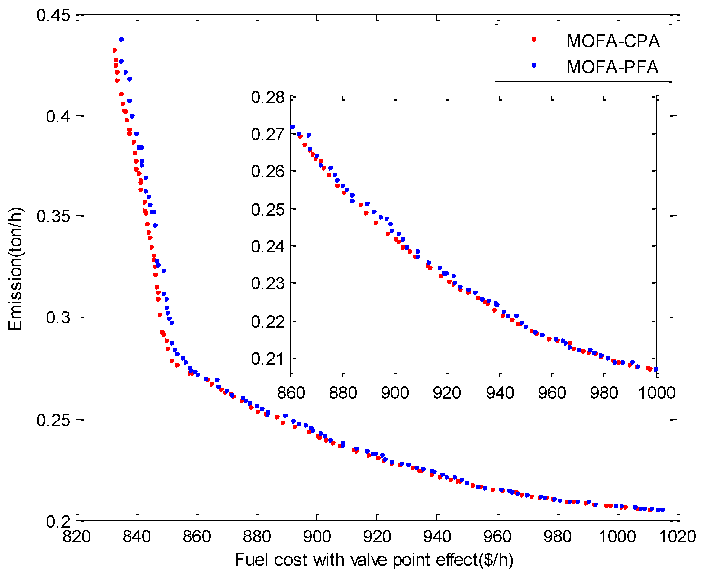
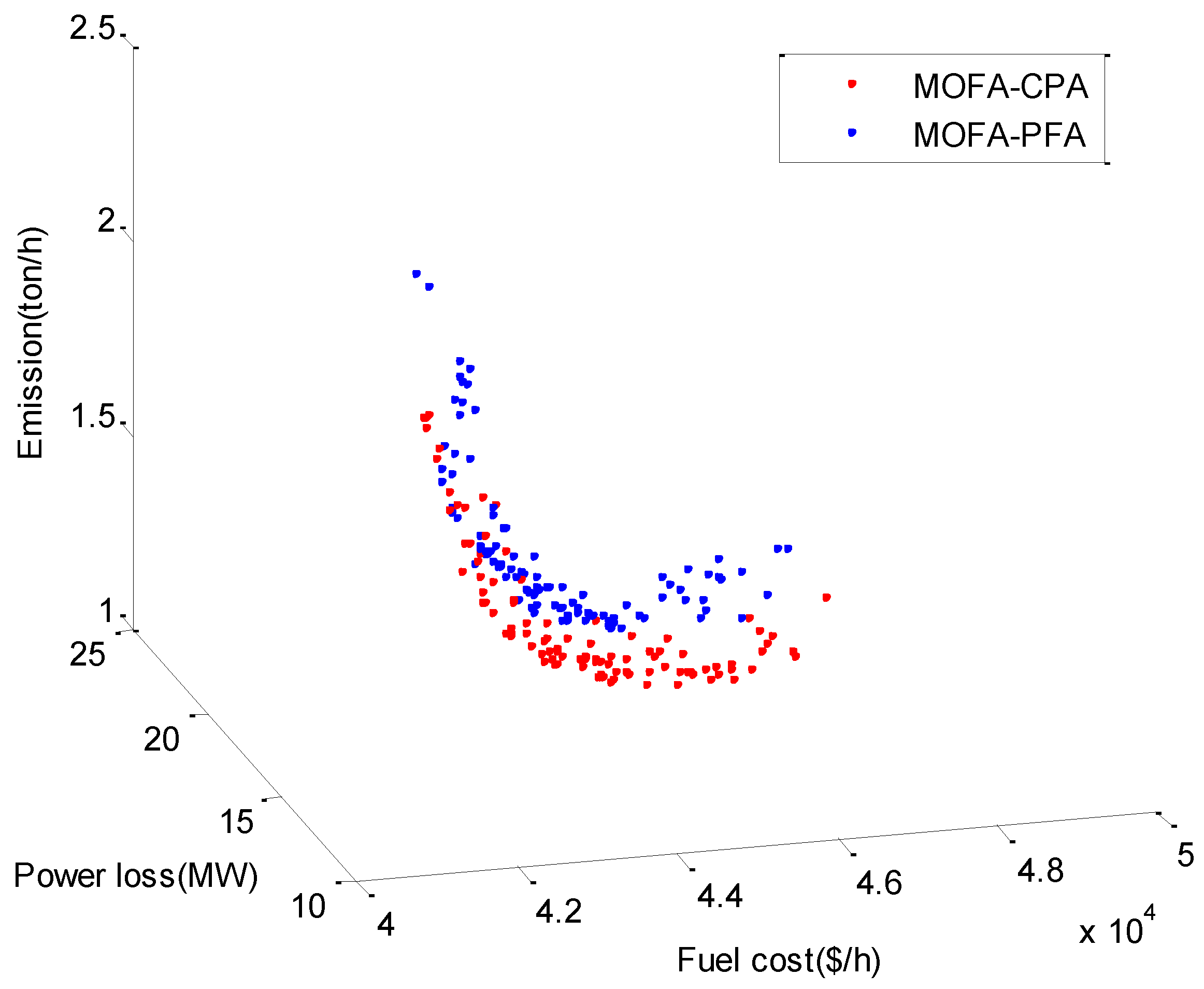
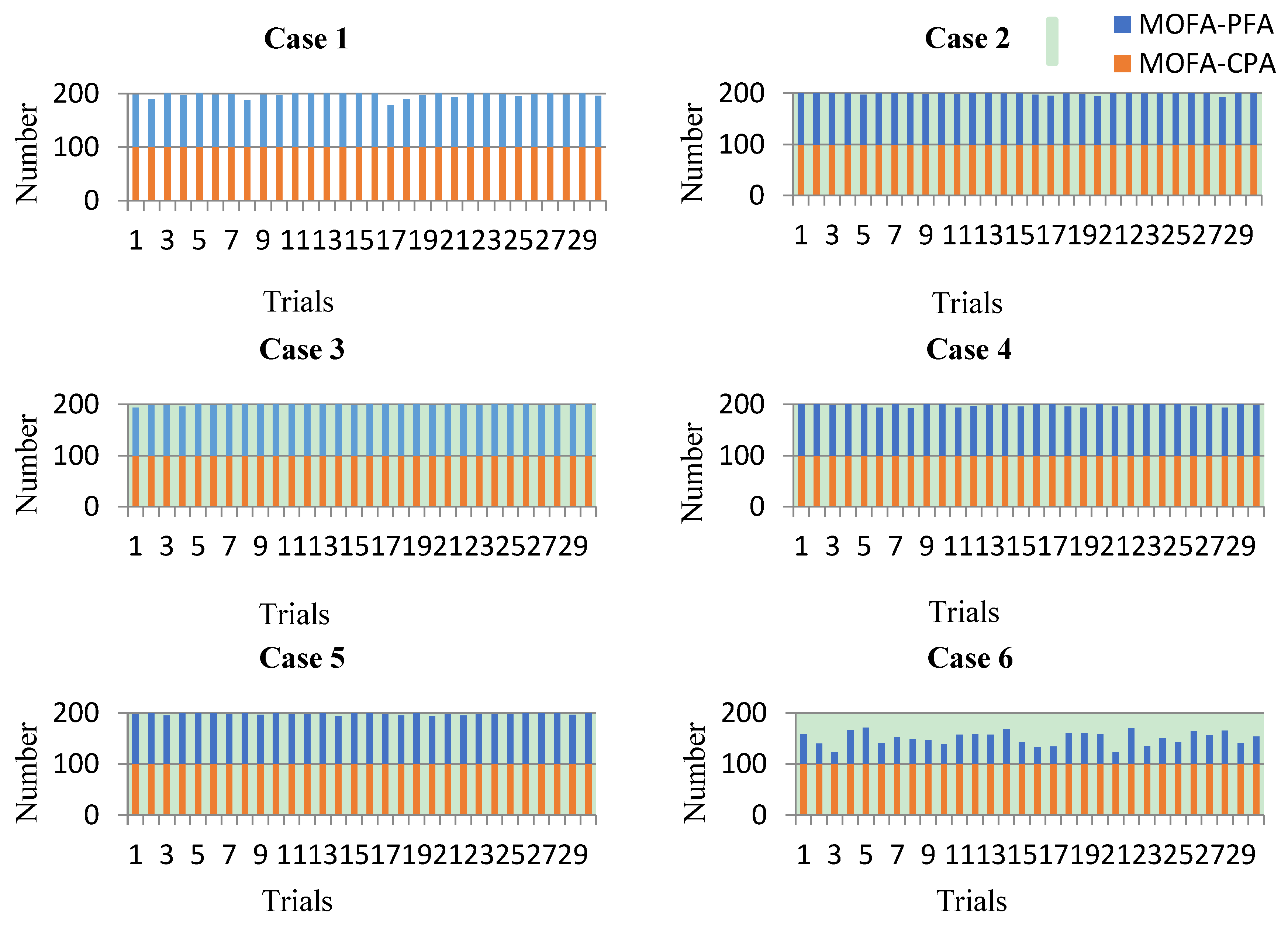
4.3. Analysis of the BCSs for Cases 1–5

The PFs found by MOFA-CPA and MOFA-PFA for the above-mentioned cases may be considered as some reference to decision-makers and smooth the selection for the appropriate best compromise solution (BCS).

Table 5. Comparisons of the BCSs found by the MOFA-CPA and MOFA-PFA algorithms for Cases 1–5.

Variables	Case 1		Case 2		Case 3		Case 4		Case 5
	Alg1 1	Alg2 2	Alg1	Alg2	Alg1	Alg2	Alg1	Alg2	Alg1	Alg2
Pg2 (MW)	52.171	54.788	53.613	49.098	64.174	57.294	57.647	57.890	61.750	59.497
Pg5 (MW)	32.314	34.118	30.305	29.139	23.342	24.599	39.791	36.290	30.736	31.945
Pg8 (MW)	35.000	34.515	34.428	35.000	34.687	33.050	35.000	35.000	35.000	34.633
Pg11 (MW)	28.381	30.000	22.187	23.853	17.439	22.333	28.504	29.271	29.457	30.000
Pg13 (MW)	22.252	25.079	13.928	17.249	15.483	18.837	35.413	40.000	27.389	27.781
Vg1 (p.u.)	1.100	1.1000	1.1000	1.1000	1.1000	1.0402	1.1000	1.0985	1.0965	1.0920
Vg2 (p.u.)	1.089	1.0936	1.0902	1.0923	1.0933	1.0262	1.0887	1.0869	1.0904	1.0848
Vg5 (p.u.)	1.063	1.0769	1.0646	1.0631	1.0804	1.0053	1.0690	1.0625	1.0687	1.0642
Vg8 (p.u.)	1.074	1.0822	1.0804	1.0811	1.0688	1.0084	1.0777	1.0767	1.0743	1.0744
Vg11 (p.u.)	1.100	1.1000	1.1000	1.0714	1.0713	1.0663	1.0951	1.0857	1.0892	1.0901
Vg13 (p.u.)	1.100	1.0894	1.1000	1.0422	1.1000	1.0668	1.0941	1.0386	1.0517	1.0413
T11 (p.u.)	0.9832	1.0160	1.0210	1.0760	0.9290	0.9780	1.0140	1.0860	1.0760	1.0730
T12 (p.u.)	0.9319	0.9650	0.9270	0.9850	1.0390	0.9920	0.9240	0.9930	0.9400	1.0030
T15 (p.u.)	1.0068	0.9960	0.9870	1.0440	1.0170	1.0560	0.9930	1.0520	0.9650	1.0400
T36 (p.u.)	0.9696	0.9710	0.9650	1.0110	1.0240	0.9690	0.9640	1.0770	0.9890	1.0200
Qc10 (p.u.)	0.0258	0.0350	0.0230	0.0060	0.0150	0.0240	0.0350	0.0140	0.0460	0.0160
Qc12 (p.u.)	0.0389	0.0000	0.0250	0.0140	0.0130	0.0240	0.0350	0.0220	0.0020	0.0110
Qc15 (p.u.)	0.0301	0.0280	0.0320	0.0170	0.0210	0.0250	0.0320	0.0080	0.0470	0.0000
Qc17(p.u.)	0.0032	0.0410	0.0110	0.0310	0.0110	0.0080	0.0120	0.0250	0.0410	0.0210
Qc20 (p.u.)	0.0407	0.0220	0.0350	0.0400	0.0310	0.0360	0.0420	0.0390	0.0340	0.0040
Qc21 (p.u.)	0.0319	0.0170	0.0050	0.0100	0.0270	0.0460	0.0080	0.0270	0.0290	0.0310
Qc23 (p.u.)	0.0225	0.0300	0.0330	0.0450	0.0400	0.0360	0.0250	0.0100	0.0060	0.0130
Qc24 (p.u.)	0.0396	0.0260	0.0480	0.0250	0.0490	0.0170	0.0460	0.0170	0.0240	0.0360
Qc29 (p.u.)	0.0243	0.0230	0.0140	0.0090	0.0390	0.0290	0.0230	0.0500	0.0220	0.0420
Fuel cost	833.94	845.01	858.50	860.37	852.02	859.47	878.13	879.91	916.59	918.57
Power loss	5.0075	4.6727	5.9031	5.9547	-	-	3.9232	4.2179	4.7780	4.7949
Emission	-	-	-	-	0.2788	0.2733	0.2161	0.2165	0.2322	0.2323

¹ MOFA-CPA; ² MOFA-PFA.

compares the best compromise solutions (BCSs) found in the Pareto front solutions related in Cases 1, 2, 3, 4, and 5, respectively. The method used to select the BCS is the fuzzy membership method described in [15].

It is clearly seen from the table that the BCS obtained by MOFA-CPA and MOFA-PFA cannot dominate each other for Case 1, while the BCS obtained by MOFA-CPA has a smaller cost value. It is also obviously seen from the table that the BCS of 858.50 $/h cost and 5.9031 MW loss achieved by MOFA-CPA for Case 2 dominates the BCS of 860.37 $/h cost and 5.9547 MW loss achieved by MOFA-PFA. For Case 3, the similar conclusions of MOFA-CPA obtaining the better BCS can still be drawn from this table. Examination of Table 5 shows that the proposed MOFA-CPA obtains all the minimum values of these three optimal objectives computed for the BCS in Case 4, and the BCS obtained by MOFA-CPA of 878.13 $/h cost, 3.9232 MW loss, and 0.2161 ton/h emission dominates the BCS obtained by MOFA-CPA of 879.91 $/h cost, 4.2179 MW loss, and 0.2165 ton/h emission. From the comparisons of obtained BCS between MOFA-CPA and MOFA-PFA for Case 5, MOFA-CPA is able to determine better solutions obtaining the lower cost with value point effect, active power loss, and emission than the MOFA-PFA method.

For the purpose of careful analysis and in-depth comparison, a comparison of objectives along with BCSs obtained by MOFA-CPA, MOFA-PFA, MOEA/D [13], NSGA-II [13], MOACSA [30], MODE [30], MOHS [31], NSGA-II [31], MOABC/D [32], MOTLA/D [32], NS_CPSO [33], SWTC_NSPSO [33], MO-DEA [34], and ICA [35] for Case 1 is given in

Table 6. Comparisons of the obtained BCS with other reported algorithms for Case 1.

Algorithms	Population Size	Maximum Iteration	Trials	Approach	Fuel Cost	Power Loss
MOFA-CPA	100	300	30	CPA	833.94	5.0075
MOFA-PFA	100	300	30	PFA	845.01	4.6727
MOEA/D [13]	100	500	31	PFA	835.36	4.9099
NSGA-II [13]	100	500	31	PFA	833.57	5.199
MOACSA [30]	50	500	-	PFA	837.7994	4.9342
MODE [30]	100	300	-	PFA	828.59	5.69
MOHS [31]	20	1000	-	-	832.6709	5.3143
NSGA-II [31]	20	1000	-	-	837.416	5.2397
MOABC/D [32]	100	1000	20	PFA	827.636	5.2451
MOTLA/D [32]	100	1000	20	PFA	826.446	5.3074
NS_CPSO [33]	100	1000	50	PFA	837.8715	4.8173
SWTC_NSPSO [33]	100	1000	50	PFA	841.1731	4.6846
MO-DEA [34]	50	300	30	PFA	820.8802	5.5949
ICA [35]	120	500	50	PFA	848.0544	4.5603

. As shown, the optimal BCS obtained by MOFA-CPA is 833.63 $/h and 5.0005 MW, which is neither too low like MODE, MOABC/D, MOTLA/D, and MO-DEA algorithms’ loss, nor too high like MOFA-PFA, MOEA/D, MOACSA, NS_CPSO, SWTC_NSPSO, and ICA algorithms’ cost, although they can get the lower loss. Since the reduction of power loss among MOFA-PFA, MOEA/D, MOACSA, SWTC_NSPSO, NS_CPSO, and ICA algorithms are around 0.3278, 0.0906, 0.0663, 0.3159, 0.1832, and 0.4402 MW, respectively, that means the fuel cost of the slack generator is needed for sustaining the incompatibility in the power system. It is quite clear that the BCS obtained by MOFA-CPA are better than other algorithms as long as the constraints are satisfied. The CPA method successfully overcomes the drawback of the traditional PFA and ensures the obtained PFs fully satisfy the inequality constraints on dependent variables.

Furthermore, a comparison of objectives along with BCSs obtained by MOFA-CPA, MOFA-PFA, MOEA/D [13], MOPSO [13], WA [36], and MOBA [36] for Case 4 is given in

Table 7. Comparisons of the obtained BCS with other reported algorithms for Case 4.

Algorithms	Population Size	Maximum Iteration	Trials	Approach	Fuel Cost	Power Loss	Emission
MOFA-CPA	100	300	30	CPA	878.13	3.9232	0.2171
MOFA-PFA	100	300	30	PFA	879.91	4.2179	0.2165
MOEA/D [13]	100	500	31	PFA	902.54	3.4594	0.2107
MOPSO [13]	100	500	31	PFA	897.48	3.9557	0.2144
WA [36]	80	300	-	-	897.2797	4.6211	0.2175

. From this table, we can notice that the MOFA-CPA can obtain better BCS in solving the tri-objective MOOPF problem, which clearly proves MOFA-CPA gives better BCS in terms of a compromise compared to other algorithms. Although the MOEA/D and MOPSO algorithms can get better emission function values, they are realized at the price of increasing the number of maximum iterations. It is worth mentioning that the comparison of MOFA-CPA between other algorithms is only given for case 1 and case 4 because no comparable literature is available for the other cases.

4.4. PF Computation of IEEE57

It is very difficult to find out the optimized solution of the tri-objective MOOPF problem for a larger power system. To extend the study, in this section, Case 6, which considers a tri-objective optimization in IEEE 57-bus test system, is analyzed. It is seen from Figure 6 that the PF obtained by MOFA-CPA are well distributed over the PF while the Pareto optimal solutions obtained by MOFA-PFA have inferior PF. Moreover, MOFA-CPA can obtain the PF of fuel cost, power loss, and emission and satisfy the inequality constraints on dependent variables. The BCSs obtained by proposed two methods are shown in

Table 8. Comparisons of the BCSs found by the MOFA-CPA and MOFA-PFA algorithms for Case 6.

Variables	Alg1 1	Alg2 2	Variables	Alg1	Alg2	variables	Alg1	Alg2
Pg2 (MW)	72.0680	90.9355	Vg9 (p.u.)	1.0696	1.0237	T58 (p.u.)	0.9820	0.9550
Pg3 (MW)	78.0025	87.0173	Vg12 (p.u.)	1.0592	1.0131	T59 (p.u.)	1.0010	0.9410
Pg6 (MW)	100.0000	100.0000	T19 (p.u.)	1.0310	0.9150	T65 (p.u.)	0.9930	0.9550
Pg8 (MW)	328.7255	334.1000	T20 (p.u.)	1.0210	0.9380	T66 (p.u.)	1.0020	0.9040
Pg9 (MW)	100.0000	100.0000	T31 (p.u.)	1.0780	1.0310	T71 (p.u.)	1.0000	0.9380
Pg12 (MW)	395.0391	406.3353	T35 (p.u.)	0.9670	0.9260	T73 (p.u.)	1.0410	0.9380
Vg1 (p.u.)	1.0784	1.0464	T36 (p.u.)	0.9810	0.9800	T76 (p.u.)	1.0090	1.0130
Vg2 (p.u.)	1.0705	1.0384	T37 (p.u.)	0.9980	1.0550	T80 (p.u.)	0.9820	1.0240
Vg3 (p.u.)	1.0686	1.0252	T41 (p.u.)	0.9810	0.9860	Qc18 (p.u.)	0.1820	0.0690
Vg6 (p.u.)	1.0717	1.0331	T46 (p.u.)	1.0010	0.9000	Qc25 (p.u.)	0.1330	0.0560
Vg8 (p.u.)	1.0750	1.0279	T54 (p.u.)	0.9020	0.9720	Qc53 (p.u.)	0.1710	0.0640
					Fuel cost	42639.96	42665.51
					Emission	11.2686	11.7785
					Power loss	1.4928	1.5234

¹ MOFA-CPA; ² MOFA-PFA.

, which testifies to that the BCS of MOFA-CPA dominates the other one.

It is worth noting that all the optimization solutions in PF obtained by MOFA-CPA shown in Figure 6 are within the permissible limits of constraints, but some optimization solutions (except for the BCS given in Table 8) in PF obtained by MOFA-PFA are beyond the permissible limits of constraints because the PFA cannot tackle constraints adequately.

4.5. Analysis of the Constraints Processing

The above analysis and presentation cannot directly show the effectiveness of the proposed CPA constraint processing method. Thus, the number of solutions satisfied constraints among 100 population size in 30 trials for all cases can be seen from Figure 7, which visually shows the performance of the proposed CPA. Also,

Table 9. Comparison of the success rate of the two algorithms for Cases 1–6.

Algorithms	Success Rate
	Case 1	Case 2	Case 3	Case 4	Case 5	Case 6
MOFA-CPA	30/30	30/30	30/30	30/30	30/30	30/30
MOFA-PFA	13/30	15/30	20/30	16/30	9/30	0/30

counts success rate (the number of trials when all solutions satisfied constraints in 30 trials) for all cases as a simple numerical example to provide an illustration of the difference between MOFA-CPA and MOFA-PFA.

Most importantly, Figure 7 reveals that CPA successfully meets the inequality constraints on dependent variables. Compared with the commonly-used PFA, CPA has a processing rate of up to 100%, especially for a larger system like the IEEE 57-bus system. Besides, the CPA not only avoids the fine tuning for the penalty factors, but also can guide the fireflies to the feasible space without delay. From this figure, we observe that the MOFA-PFA is very unsuitable in solving several MOOPF problems with different complexities, such as Case 6. For Cases 1–6, MOFA-PFA cannot guarantee that all inequality constraints are within the permissible limits in each trial, while MOFA-CPA has the success rate of 30/30 in each trial which can be seen from Table 9.

4.6. Performance Evaluation

In order to show the effect of 30 trials, a statistical analysis of 30 trials is performed with the following two types of commonly-used indicators, SPREAD [20,37,38] and HV [39,40].

Table 10. The statistical results of HV and SPREAD of the two algorithms for Cases 1–6.

Algorithm	Quality Indictor		Case 1	Case 2	Case 3	Case 4	Case 5	Case 6
MOFA-CPA	HV	Mean	759.14	1060.53	35.32	110.96	205.93	602,013.21
		Std	6.93	8.22	0.43	0.54	3.16	53,158.19
	SPREAD	Mean	0.74	0.73	0.88	0.76	0.77	0.73
		Std	0.02	0.02	0.02	0.03	0.04	0.03
MOFA-PFA	HV	Mean	739.70	1050.39	35.09	88.33	204.07	598,973.46
		Std	6.93	7.62	0.39	3.69	3.66	54,066.57
		p	1.73 × 10−6	5.75 × 10−6	0.0495	1.73 × 10−6	0.0571	0.6733
		h	1	1	1	1	0	0
	SPREAD	Mean	0.85	0.86	0.89	0.94	0.79	0.83
		Std	0.01	0.01	0.02	0.02	0.04	0.02
		p	1.73 × 10−6	1.73 × 10−6	0.2369	1.73 × 10−6	0.0687	1.73 × 10−6
		h	1	1	0	1	0	1

shows the statistical results of the proposed MOFA-CPA and MOFA-PFA in 30 trials for test Cases 1–6. This table includes the mean and standard deviation of the SPREAD and HV for the two algorithms in order to reflect a numerical comparison. The statistical results of Wilcoxon signed rank test for SPREAD and HV between the proposed MOFA-CPA and MOFA-PFA in 30 trials are simultaneously shown in Table 10. The Wilcoxon signed rank test has been tested at the 0.05 significance level, where, p is the probability of observing a test statistic, h is a logical value. h = 1 indicates that the standard results between the proposed MOFA-CPA and MOFA-PFA are quite different. h = 0 indicates that the standard results between the proposed MOFA-CPA and MOFA-PFA are similar.

From the results in Table 10, it can be seen that the mean HV of the MOFA-CPA algorithm is significantly better than the results obtained from MOFA-PFA algorithm for all cases, which shows that PFs obtained by MOFA-CPA are closer to the true PF. It also shows that the distribution of the proposed algorithm has better distribution uniformity than the distribution of the MOFA-PFA algorithm. At the same time, it can also be seen that the MOFA-CPA algorithm outperforms the MOFA-PFA algorithm both in terms of convergence, distribution, and breadth due to the lower mean SPREAD. Furthermore, the difference between the proposed MOFA-CPA and MOFA-PFA is significant in Cases 1, 2, 3, 4, and 6.

Table 11. Comparison of mean CPU time of two algorithms for Cases 1–6.

Algorithms	Mean CPU Time (sec)/Tmax
	Case 1	Case 2	Case 3	Case 4	Case 5	Case 6
MOFA-CPA	145.93/300	166.53/300	168.71/300	315.21/500	332.13/500	519.25/500
MOFA-PFA	153.74/300	169.68/300	170.38/300	319.54/500	336.14/500	525.12/500

sums up the mean CPU time of the two algorithms for Cases 1–6. In all cases, the mean CPU times of the proposed MOFA-CPA are slightly smaller than those of the MOFA-PFA method, and the IEEE 57-bus system needs more time to find PFs because it is larger than the IEEE 30-bus system. It shows that incorporation of the valve-point effect in Case 2, Case 3, and Case 5 needs more computation time.

5. Conclusions

Researchers have encountered great difficulties in handling the inequality constraints of dependent variables when dealing with large-scale, multi-constrained MOOPF problems. Many published studies have adopted the commonly-used PFA to handle constraints, which spends much time on the fine tuning of the penalty factors and the handling effect is not perfect. For this reason, the multi-objective firefly algorithm with a constraints-prior Pareto-domination approach (MOFA-CPA) is proposed in this paper. CPA is proposed for ensuring non-violation of various inequality constraints on dependent variables by introducing the Pareto-domination principle based on the sum of constraint violations. With the purpose of demonstrating the feasibility of the proposed method, two systems (the IEEE 30-bus and the IEEE 57-bus system) and six different cases are considered for the MOOPF problem. The results obtained by the MOFA-CPA are compared with MOFA-PFA and other methods proposed in recent publications, and the simulation results indicate that the BCS obtained by MOFA-CPA is better than other algorithms as long as the constraints are satisfied. The analysis of the constraints processing shows that the CPA method successfully overcomes the drawback of the traditional PFA and ensures the obtained PFs fully satisfy the inequality constraints of the dependent variables.

References

1. Chen, G.; Liu, L.; Song, P.; Du, Y. Chaotic improved PSO-based multi-objective optimization for minimization of power losses and L index in power systems. Energy Convers. Manag. 2014, 86, 548–560. [Google Scholar] [CrossRef]
2. Zhou, J.; Xu, Y.; Zheng, Y.; Zhang, Y. Optimization of Guide Vane Closing Schemes of Pumped Storage Hydro Unit Using an Enhanced Multi-Objective Gravitational Search Algorithm. Energies 2017, 10, 911. [Google Scholar] [CrossRef]
3. Amrane, Y.; Boudour, M.; Ladjici, A.A.; Elmaouhab, A. Optimal VAR control for real power loss minimization using differential evolution algorithm. Int. J. Electr. Power Energy Syst. 2015, 66, 262–271. [Google Scholar] [CrossRef]
4. Biswas, P.P.; Suganthan, P.N.; Mallipeddi, R.; Amaratunga, G.A.J. Optimal power flow solutions using differential evolution algorithm integrated with effective constraint handling techniques. Eng. Appl. Artif. Intell. 2018, 68, 81–100. [Google Scholar] [CrossRef]
5. Elsaiah, S.; Cai, N.; Benidris, M.; Mitra, J. Fast economic power dispatch method for power system planning studies. IET Gener. Transm. Distrib. 2015, 9, 417–426. [Google Scholar] [CrossRef]
6. Bhowmik, A.R.; Chakraborty, A.K. Solution of optimal power flow using nondominated sorting multi objective gravitational search algorithm. Int. J. Electr. Power Energy Syst. 2014, 62, 323–334. [Google Scholar] [CrossRef]
7. Chaib, A.E.; Bouchekara, H.R.E.H.; Mehasni, R.; Abido, M.A. Optimal power flow with emission and non-smooth cost functions using backtracking search optimization algorithm. Int. J. Electr. Power Energy Syst. 2016, 81, 64–77. [Google Scholar] [CrossRef]
8. Warid, W.; Hizam, H.; Mariun, N.; Abdul-Wahab, N. Optimal Power Flow Using the Jaya Algorithm. Energies 2016, 9, 678. [Google Scholar] [CrossRef]
9. He, X.; Wang, W.; Jiang, J.; Xu, L. An Improved Artificial Bee Colony Algorithm and Its Application to Multi-Objective Optimal Power Flow. Energies 2015, 8, 2412–2437. [Google Scholar] [CrossRef] [Green Version]
10. Niknam, T.; Narimani, M.R.; Jabbari, M.; Malekpour, A.R. A modified shuffle frog leaping algorithm for multi-objective optimal power flow. Energy 2011, 36, 6420–6432. [Google Scholar] [CrossRef]
11. Sahu, S.; Barisal, A.K.; Kaudi, A. Multi-objective optimal power flow with DG placement using TLBO and MIPSO: A comparative study. Energy Procedia 2017, 117, 236–243. [Google Scholar] [CrossRef]
12. Kim, H.-Y.; Kim, M.-K.; Kim, S. Multi-Objective Scheduling Optimization Based on a Modified Non-Dominated Sorting Genetic Algorithm-II in Voltage Source Converter−Multi-Terminal High Voltage DC Grid-Connected Offshore Wind Farms with Battery Energy Storage Systems. Energies 2017, 10, 986. [Google Scholar] [CrossRef]
13. Zhang, J.; Tang, Q.; Li, P.; Deng, D.; Chen, Y. A modified MOEA/D approach to the solution of multi-objective optimal power flow problem. Appl. Soft Comput. 2016, 47, 494–514. [Google Scholar] [CrossRef]
14. Yu, W.-J.; Ji, J.-Y.; Gong, Y.-J.; Yang, Q.; Zhang, J. A tri-objective differential evolution approach for multimodal optimization. Inf. Sci. 2018, 423, 1–23. [Google Scholar] [CrossRef]
15. Barocio, E.; Regalado, J.; Cuevas, E.; Uribe, F.; Zúñiga, P.; Torres, P.J.R. Modified bio-inspired optimisation algorithm with a centroid decision making approach for solving a multi-objective optimal power flow problem. IET Gener. Transm. Distrib. 2017, 11, 1012–1022. [Google Scholar] [CrossRef]
16. Bhowmik, A.R.; Chakraborty, A.K.; Babu, K.N. Multi objective optimal power flow using NSMOGSA. In Proceedings of the 2014 International Conference on Circuits, Power and Computing Technologies [ICCPCT], Nagercoil, India, 20–21 March 2014; pp. 84–88. [Google Scholar]
17. Sedighizadeh, M.; Bakhtiary, R. Optimal multi-objective reconfiguration and capacitor placement of distribution systems with the Hybrid Big Bang–Big Crunch algorithm in the fuzzy framework. Ain Shams Eng. J. 2016, 7, 113–129. [Google Scholar] [CrossRef]
18. Mohamed, A.-A.A.; Mohamed, Y.S.; El-Gaafary, A.A.M.; Hemeida, A.M. Optimal power flow using moth swarm algorithm. Electr. Power Syst. Res. 2017, 142, 190–206. [Google Scholar] [CrossRef]
19. Chaine, S.; Tripathy, M.; Jain, D. Non dominated Cuckoo search algorithm optimized controllers to improve the frequency regulation characteristics of wind thermal power system. Eng. Sci. Technol. Int. J. 2017, 20, 1092–1105. [Google Scholar] [CrossRef]
20. Deb, K.; Pratap, A.; Agarwal, S.; Meyarivan, T. A fast and elitist multiobjective genetic algorithm: NSGA-II. IEEE Trans. Evol. Comput. 2002, 6, 182–197. [Google Scholar] [CrossRef] [Green Version]
21. Rezaei Adaryani, M.; Karami, A. Artificial bee colony algorithm for solving multi-objective optimal power flow problem. Int. J. Electr. Power Energy Syst. 2013, 53, 219–230. [Google Scholar] [CrossRef]
22. Kumari, M.S.; Maheswarapu, S. Enhanced Genetic Algorithm based computation technique for multi-objective Optimal Power Flow solution. Int. J. Electr. Power Energy Syst. 2010, 32, 736–742. [Google Scholar] [CrossRef]
23. Chen, H.; Bo, M.L.; Zhu, Y. Multi-hive bee foraging algorithm for multi-objective optimal power flow considering the cost, loss, and emission. Int. J. Electr. Power Energy Syst. 2014, 60, 203–220. [Google Scholar] [CrossRef]
24. Warid, W.; Hizam, H.; Mariun, N.; Abdul Wahab, N.I. A novel quasi-oppositional modified Jaya algorithm for multi-objective optimal power flow solution. Appl. Soft Comput. 2018, 65, 360–373. [Google Scholar] [CrossRef]
25. Chen, G.; Yi, X.; Zhang, Z.; Wang, H. Applications of multi-objective dimension-based firefly algorithm to optimize the power losses, emission, and cost in power systems. Appl. Soft Comput. 2018, 68, 322–342. [Google Scholar] [CrossRef]
26. Verma, O.P.; Aggarwal, D.; Patodi, T. Opposition and dimensional based modified firefly algorithm. Expert Syst. Appl. 2016, 44, 168–176. [Google Scholar] [CrossRef]
27. Wang, H.; Wang, W.; Zhou, X.; Sun, H.; Zhao, J.; Yu, X.; Cui, Z. Firefly algorithm with neighborhood attraction. Inf. Sci. 2017, 382–383, 374–387. [Google Scholar] [CrossRef]
28. Deo, R.C.; Ghorbani, M.A.; Samadianfard, S.; Maraseni, T.; Bilgili, M.; Biazar, M. Multi-layer perceptron hybrid model integrated with the firefly optimizer algorithm for windspeed prediction of target site using a limited set of neighboring reference station data. Renew. Energy 2018, 116, 309–323. [Google Scholar] [CrossRef]
29. Roy, P.; Roy, P.; Chakrabarti, A. Modified shuffled frog leaping algorithm with genetic algorithm crossover for solving economic load dispatch problem with valve-point effect. Appl. Soft Comput. 2013, 13, 4244–4252. [Google Scholar] [CrossRef]
30. Rao, B.S.; Vaisakh, K. Application of ACSA for solving multi-objective optimal power flow problem with load uncertainty. In Proceedings of the 2013 IEEE International Conference on Emerging Trends in Computing, Communication and Nanotechnology (ICECCN), Tirunelveli, India, 25–26 March 2013; pp. 764–771. [Google Scholar]
31. Sivasubramani, S.; Swarup, K.S. Multi-objective harmony search algorithm for optimal power flow problem. Int. J. Electr. Power Energy Syst. 2011, 33, 745–752. [Google Scholar] [CrossRef]
32. Medina, M.A.; Das, S.; Coello Coello, C.A.; Ramírez, J.M. Decomposition-based modern metaheuristic algorithms for multi-objective optimal power flow—A comparative study. Eng. Appl. Artif. Intell. 2014, 32, 10–20. [Google Scholar] [CrossRef]
33. Man-Im, A.; Ongsakul, W.; Singh, J.G.; Boonchuay, C. Multi-objective optimal power flow using stochastic weight trade-off chaotic NSPSO. In Proceedings of the 2015 IEEE Innovative Smart Grid Technologies—Asia (ISGT ASIA), Bangkok, Thailand, 3–6 November 2015; pp. 1–8. [Google Scholar]
34. Shaheen, A.M.; El-Sehiemy, R.A.; Farrag, S.M. Solving multi-objective optimal power flow problem via forced initialised differential evolution algorithm. IET Gener. Transm. Distrib. 2016, 10, 1634–1647. [Google Scholar] [CrossRef]
35. Ghasemi, M.; Ghavidel, S.; Ghanbarian, M.M.; Gharibzadeh, M.; Azizi Vahed, A. Multi-objective optimal power flow considering the cost, emission, voltage deviation and power losses using multi-objective modified imperialist competitive algorithm. Energy 2014, 78, 276–289. [Google Scholar] [CrossRef]
36. Sumetha, A.; Pornrapeepat, B. A multi-objective bees algorithm for multi-objective optimal power flow problem. In Proceedings of the 8th International Conference on Electrical Engineering/Electronics, Computer, Telecommunications and Information Technology (ECTI-CON), Khon Kaen, Thailand, 17–19 May 2011; pp. 852–856. [Google Scholar]
37. Deb, K.; Jain, H. An Evolutionary Many-Objective Optimization Algorithm Using Reference-Point-Based Nondominated Sorting Approach, Part I: Solving Problems With Box Constraints. IEEE Trans. Evol. Comput. 2014, 18, 577–601. [Google Scholar] [CrossRef]
38. Narimani, M.R.; Azizipanah-Abarghooee, R.; Zoghdar-Moghadam-Shahrekohne, B.; Gholami, K. A novel approach to multi-objective optimal power flow by a new hybrid optimization algorithm considering generator constraints and multi-fuel type. Energy 2013, 49, 119–136. [Google Scholar] [CrossRef]
39. While, L.; Bradstreet, L.; Barone, L. A Fast Way of Calculating Exact Hypervolumes. IEEE Trans. Evol. Comput. 2012, 16, 86–95. [Google Scholar] [CrossRef]
40. While, L.; Hingston, P.; Barone, L.; Huband, S. A faster algorithm for calculating hypervolume. IEEE Trans. Evol. Comput. 2006, 10, 29–38. [Google Scholar] [CrossRef] [Green Version]
Figure 1. Pareto fronts (PFs) obtained by MOFA-CPA and MOFA-PFA for Case 1.
Energies 11 03438 g001
Figure 2. PFs obtained by MOFA-CPA and MOFA-PFA for Case 2.
Energies 11 03438 g002
Figure 3. PFs obtained by MOFA-CPA and MOFA-PFA for Case 3.
Energies 11 03438 g003
Figure 4. PFs obtained by MOFA-CPA and MOFA-PFA for Case 4.
Energies 11 03438 g004
Figure 5. PFs obtained by MOFA-CPA and MOFA-PFA for Case 5.
Energies 11 03438 g005
Figure 6. PFs obtained by MOFA-CPA and MOFA-PFA for Case 6.
Energies 11 03438 g006
Figure 7. The number of solutions with satisfied constraints in all cases with population size of 100.
Energies 11 03438 g007