Simulation-Based Evaluation and Optimization of Control Strategies in Buildings

Abstract

Over the last several years, a great amount of research work has been focused on the development of model predictive control techniques for the indoor climate control of buildings, but, despite the promising results, this technology is still not adopted by the industry. One of the main reasons for this is the increased cost associated with the development and calibration (or identification) of mathematical models of special structure used for predicting future states of the building. We propose a methodology to overcome this obstacle by replacing these hand-engineered mathematical models with a thermal simulation model of the building developed using detailed thermal simulation engines such as EnergyPlus. As designing better controllers requires interacting with the simulation model, a central part of our methodology is the control improvement (or optimisation) module, facilitating two simulation-based control improvement methodologies: one based in multi-criteria decision analysis methods and the other based on state-space identification of dynamical systems using Gaussian process models and reinforcement learning. We evaluate the proposed methodology in a set of simulation-based experiments using the thermal simulation model of a real building located in Portugal. Our results indicate that the proposed methodology could be a viable alternative to model predictive control-based supervisory control in buildings.

1. Introduction

Building Management Systems (BMSs) provide monitoring and control capability for multiple sub-systems including Heating, Ventilation and Air Conditioning (HVAC). Modern BMSs additionally offer some energy management functionality based on a set of low-level controllers, such as thermostats. Up to 20% of the energy used for HVAC and lighting system operation is lost due to poor configuration of such controllers or due to equipment faults [1]. Even in the case of good controller configurations, it is very hard to encapsulate efficient control strategies within a static set of simple rules, especially in large buildings with complex energy or renewable systems installed; here, all generation, distribution and room-level systems need to operate in a coordinated manner and be able to adapt to stochastic generation patterns that strongly depend on weather conditions [2].

Recently, this manual configuration and control tuning process has been replaced by a methodology developed following two axes [2,3]:

• Utilise predictions instead of historical data: Here, instead of gathering and analysing historical data from the building to improve the efficiency of specific controllers, forecasts (e.g., on weather, occupancy, equipment gains, etc.) are utilised to determine the (near-)future state (e.g., thermal/visual comfort conditions) of the building. This can enable for a continuous adaptation of the control logic to the (predicted) needs of the building and the microclimatic conditions of each site.
• Automated controller tuning: Here, an optimisation process is defined (utilising the available predictions) to design efficient controllers in an automated and laborious-free manner.

This approach has been made possible by two key technologies: (i) the application of Model Predictive Control (MPC) paradigm in buildings (e.g., see [2,3,4,5,6,7,8,9,10,11,12,13,14]); and (ii) the development of scalable BMS, e.g., the Johnson’s Controls METASYS^®, which provide a remote (cloud-based) layer for hosting computationally demanding services, such as supervisory-level control design.

In MPC application in buildings, typically, we assume that a model of the controlled process (i.e., the real building in our case) as well as (weather, occupancy, etc.) forecasts for a predefined time window are available. This way, a constrained optimisation problem can be formulated and solved for a predefined period in the future, generating a control signal (or control strategy) which is optimised for the system on the basis of a defined cost function and a set of (visual, thermal, air-quality, etc.) comfort constraints. The quality of the final control strategy is evaluated under a set of Key Performance Indicators (KPIs). A high-level schematic of the overall approach is shown in Figure 1.

Despite the fact that MPC for building energy management and indoor climate regulation has been an active research topic, a plethora of research work has been published in the field and impressive results in real-world and simulated applications have been reported in relevant projects and publications, it has really not found its way into the market. Very few companies include some simple aspects of MPC in their offerings [15,16] and these implementations are far from being fully-fledged MPC solutions. This hesitation of companies to include MPC in their product lines cannot be only attributed to conservatism on the side of the industry; some of the mechanics of MPC violate specific needs of building owners and operators.

One of the biggest obstacles towards market adoption is that MPC requires a model of the building [2], usually of a very specific linear or bi-linear structure [3,17,18,19,20,21]. In addition, in holistic use cases, all involved generation and distribution systems need to be modelled too [21,22]—and there have been only few notable efforts for model standardisation (e.g., see [23,24]).

Model development induces the largest monetary costs in MPC applications [6], but what has been rather overlooked is that there are several other practical steps towards deploying MPC in a real building that also yield increased costs:

• installing additional sensors/meters required for accurate state estimation of the building to minimise the model/reality mismatch;
• configuration of the overall MPC solution (including model calibration) requires significant amount of time and the involvement of high-qualified engineers; and
• monitoring and solution debugging times of MPC solutions are significantly higher compared to the deployment of traditional knowledge-based controllers.

In several cases, the achieved cost savings might not be high enough to achieve a favourable Return of Investment (ROI) [6].

In addition, as analysed in [2,25], there is a cost (e.g., express as productivity loss [26,27]) associated with the inability of most MPC-oriented bi-linear models to accurately estimate occupant thermal sensation, e.g., under the guidelines of ISO 7730 [28] or ASHRAE 55 [29], as most MPC applications in buildings define room thermal comfort as a pre-defined region of air [30] or operative [3] temperatures with only few exceptions [31,32,33,34]. This limitation becomes more restricting as personalised thermal comfort models [35,36,37,38,39] have increasingly started becoming the norm.

In an effort to overcome these limitations, we propose a methodology that utilises Building Energy Performance (BEP) simulation models, developed using BEP simulation engines such as EnergyPlus [40] or Modelica [41] in place of the purpose-built models for MPC. A standardised automatic creation of BEP simulation models could expedite the BEP simulation modelling process, making it more cost-effective and less vulnerable to modelling errors. To this direction, the automated data transformation from Building Information Models (BIM) data to input data of thermal simulation tools has received considerable attention recently [42,43,44,45,46,47]. Concerning the BIMs availability, regulatory requirements and technological advances in the field of building information modelling are resulting in increased adoption and availability of BIM data. At the same time, BIM-based workflows are increasingly adopted in professional practice, which has resulted on comprehensive and usable BIM models’ availability. Hence, adoption of such an automated BEP simulation models’ generation from BIM data is not far into the future (see [48] and the references therein for a thorough review and algorithmic implementations).

Even though other model-assisted control design approaches have also used these types of models, the novelty of our work lies in the methods we define for generating optimised control strategies through interacting with the model: (i) simulation-based evaluation using multi-criteria decision analysis methods; and (ii) simulation-based optimisation using Gaussian process state space models. Our proposed approach combines ideas from multi-criteria decision theory and both the data-driven control [49,50,51] and reinforcement learning [52,53,54] domains and is evaluated as a proof-of-concept utilising the simulation model of a real building located in Portugal.

The remainder of this paper is structured as follows: Section 2 provides an overview of the MPC methodology in buildings; Section 3 describes the proposed methodology; Section 4 presents the experimental setup and the main results; and Section 5 presents the final conclusions and concrete next steps towards future work.

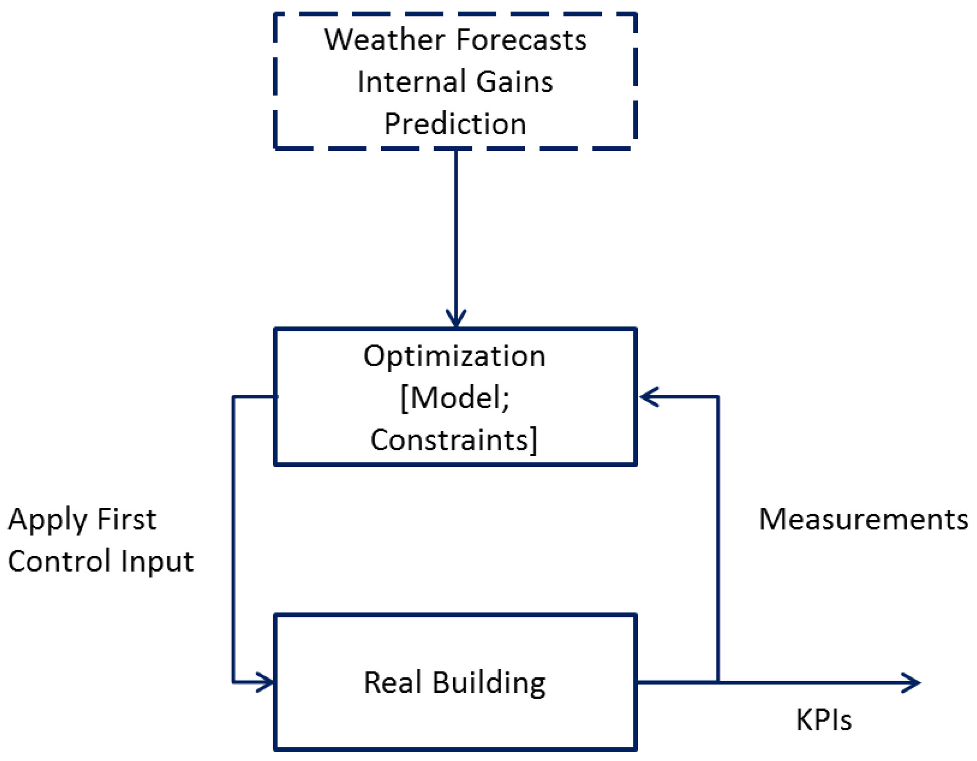
2. Model Predictive Control in Buildings

A more formal definition of the MPC formulation can be seen in the following Equation [3,4]:

$$\begin{array}{c}{\mathbf{u}}^{\ast }=\underset{u\in \mathbb{U}}{argmin}\sum _{t=1}^T{g}_t(x_t,u_t,w_t)\hfill \\ \mathrm{subject}\mathrm{to}:\hfill \\ x_{t+1}=f(x_t,u_t,w_t)\hfill \\ u_t\in \mathbb{U}\hfill \\ x_t\in \mathbb{X}\hfill \\ w_t\in \mathbb{W}\hfill \\ C\left(x_t\right)\le 0.\hfill \end{array}$$

(1)

Here, we have the following:

• t is the discrete time-step (with its length depending on the application), T is the prediction horizon.
• ${\mathbf{u}}^{\ast }:=\left[u_1,u_2,\dots ,u_T\right]$ is the optimal control solution.
• $x_t$ is a vector of values for each time-step t for the states of the system (e.g., wall and air temperatures [3]).
• The admissible control actions $u_t$ are a vector of values for each time-step t, with each value corresponding to a control action (e.g., temperature set-point, hot water flow, etc.) for all controllable systems of the building.
• $w_t$ is a vector of exogenous, uncontrollable factors affecting the system, like weather conditions or user actions. As discussed previously, we have some (reliable) predictions ${\widehat{w}}_t$ for these disturbances.
• $\mathbb{U}\subseteq {\mathbb{R}}^m$ and $\mathbb{X}\subseteq {\mathbb{R}}^n$ are closed sets defining the admissible controls and states respectively, while $\mathbb{W}\subseteq {\mathbb{R}}^v$ is the closed set of exogenous uncorrelated factors.
• $f:{\mathbb{R}}^{(n+v)}\times {\mathbb{R}}^m\to {\mathbb{R}}^n$ is a (possibly non-linear) function that describes the system dynamics.
• $g_t\in \mathbb{R}$ is the value of the cost (or objective) function to be minimised at time t and represents a performance measure, estimating the efficiency of a given control strategy. In the buildings domain, this index can either be economical (e.g., minimise operational cost) or environmental (e.g., maximise the net energy produced or minimise CO${}_2$ emissions).
• $C\left(x_t\right)\le 0$ is a function usually describing thermal comfort constraints for the building occupants.

To account for modelling/prediction errors, only the first control action is applied to the building and the whole process re-initiates.

Starting from this generic definition, we can distinguish different categories of MPC algorithms for buildings, depending on the type of model used and the associated optimisation approach for solving the defined constrained optimisation problem. In the remainder of this section, we provide a high-level overview of these categories, but a detailed analysis is beyond the scope of this paper. We refer the interested reader to [2,5] and the references therein for a thorough analysis.

Physics-based models These models are designed based on first principles, utilising knowledge of the underlying physical process of the building and are usually analogous to electrical Resistance–Capacitance (RC) networks [3,6,17,18,19,20,21]. In an effort to reduce the model design- and calibration-associated costs for these models, a number of MPC approaches based on system identification methods [18,50,51,55,56,57,58] have been proposed. The problem here is that some initial (quasi-)random actions need to be performed to the real building (called persistent excitation signals in system identification theory) [51,56,59,60] to satisfy key theoretical assumptions on reliable statistical identification [55,61]. In real operation, this requirement is almost always infeasible without compromising the comfort or the health of the occupants (note that this is a problem closely related to the safe exploration/exploitation dilemma that has been extensively studied in reinforcement learning [52,53,62,63]). It is conceivable that a poorly identified model can lead to severe compromise of occupant comfort conditions; the model will provide inaccurate predictions that will lead to unsuitable controllers [64].

Data-driven models Here, a linear or non-linear regression model is fitted using available data from the real building and then utilised for the MPC application. Several types of regression functions have been reported in the literature, e.g. neural networks, support vector regression, autoregressive moving average, regression trees, etc. (see [5,65] for an overview). These models have the same data requirements as the system identification methods described before while they also suffer from poor extrapolation properties.

BEP simulation models When these models are utilised for control design, the main concern is the optimisation algorithm to be used, as they are characterised by high simulation times. A common approach is to assume that the simulation model is an exact model of the real building and construct a surrogate regression model off-line; this model is orders of magnitude faster compared to the original model so it could be used for MPC-like on-line control design [55,66]. From our experience with real-building control experiments [2,4,67], the assumption that the original simulation model (and thus also the surrogate model derived from it) can actually predict all states of the real building, under all different combinations of weather conditions and occupant actions, usually does not hold in practice. Instead, what is required is a continuous calibration process, for example as defined in the digital twin paradigm [68].

A second approach that has been reported to address the sample complexity problem is to directly replace the (bi-)linear model required in classical MPC with the detailed thermal simulation model. Early work here [69,70] has used global constrained optimisation approaches (such as genetic algorithms), but as the number of required simulation calls is quite high (and would grow exponentially with the number of posed comfort constraints [70]), these algorithms would scale poorly in realistic building control scenarios.

More recent work in the same direction [2,4,67,71,72,73,74] uses the available simulation model to construct a simple meta-model of the building online, which is able to predict the behavior of the building only for a limited prediction horizon. This meta-model is used for the optimisation of the control strategy, in an effort to reduce the number of simulation calls to the “expensive" simulation model. The problem with most approaches here stems from the multi-objective formulation of the optimisation algorithm [2,4,71], in which the objective function to be optimised is a properly weighted combination of a cost function (e.g., the total energy consumption) and a term that expresses the thermal discomfort for the entire building (in most cases, average discomfort values for all offices are calculated, in contrast to normative guidelines [28,75]). In large-scale real-world setups, hand-tuning a proper weighting between the active constraints being generic enough to capture all the real-world variations (e.g., varying daily weather conditions, occupant actions, etc.) is a formidable task. For example, in an office building with 30 offices, where thermal and visual comfort constraints need to be met, minimising the energy consumption of the building while giving priority to thermal over visual comfort constraints requires: (i) proper normalisation between the energy consumption, the thermal comfort and visual comfort constraints values so no term is dominating the combined cost function [76]; and (ii) adjusting the relative importance of visual over thermal comfort constraints Finally, constrained Bayesian optimisation has been used to address these shortcomings [2], but, even though this approach resulted in a successful real-world application, Bayesian optimisation does not scale well in problems with a high number of optimisation parameters [77].

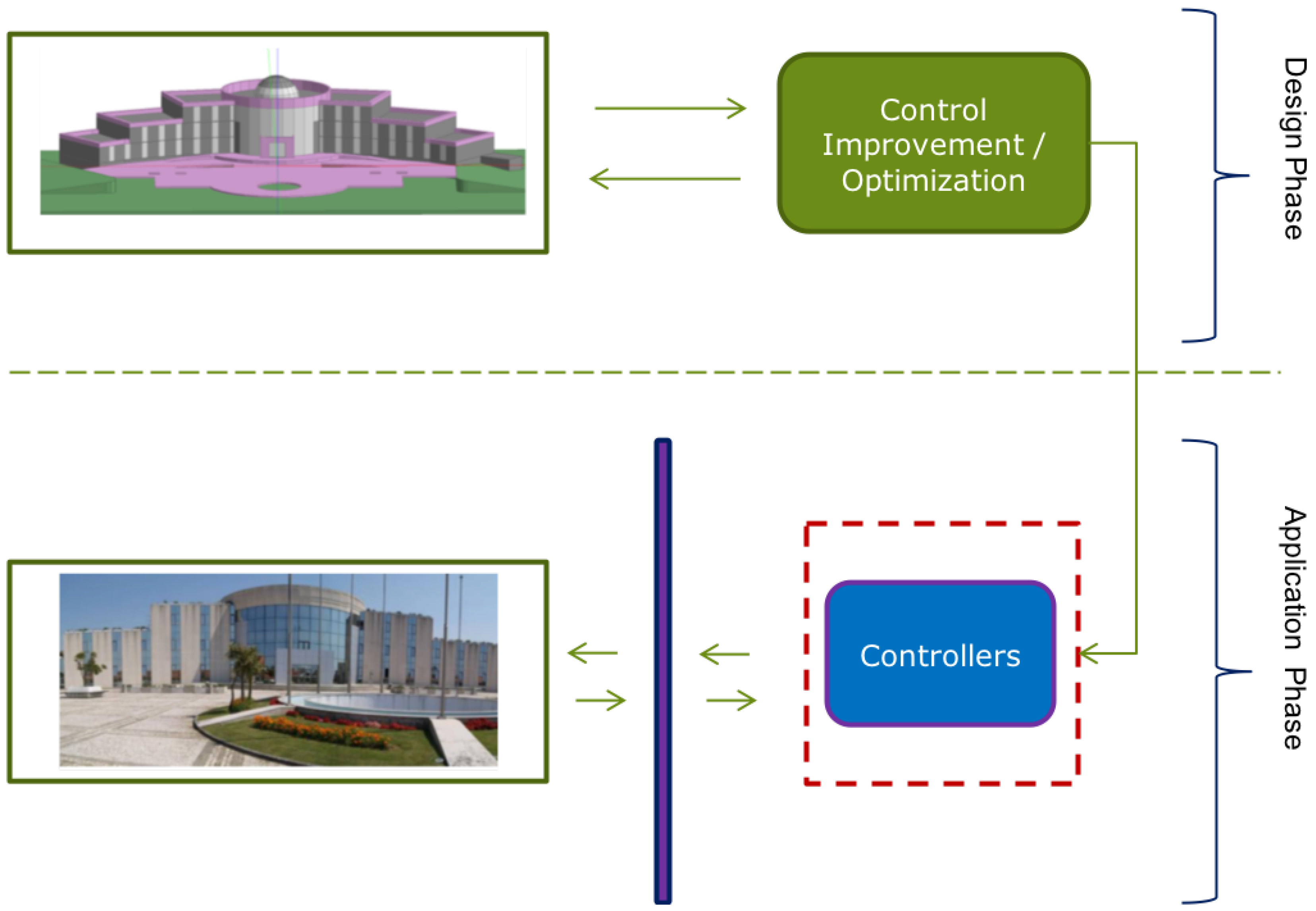
3. The Proposed Approach

Taking into account all the above, in the present work, we define a methodology that builds upon some of the ideas that enable the great potential of MPC, but at the same time satisfies the requirements of building owners on reduced cost and more transparent control decisions [78]. To achieve this, in the heart of our methodology lies a set of Building Energy Performance (BEP) simulation models, developed to use BEP simulation engines such as EnergyPlus or Modelica, instead of using purpose-built models for every study building.

Here, we utilise the simulation model in an on-line fashion, but we deviate from previous work by developing and evaluating two simulation-based control improvement/optimisation methods (analysed in the remainder of this section): (i) simulation-based evaluation using multi-criteria decision analysis methods; and (ii) simulation-based optimisation using Gaussian process state space models. The high-level view of the overall methodology—which is similar to the classical MPC work flow—is shown in Figure 2, where we have the following steps:

• Design Phase:
  • The Control Improvement module evaluates candidate control strategies utilising the simulation model under a set of pre-defined objectives (e.g., energy consumption, thermal comfort in each controller space, etc).
  • When the Design Phase finishes, the best resulting strategy is communicated and deployed to the real building.
• Application Phase:
  • The deployed controllers are used to generate new control actions in each control time-step for each controllable system of the building (possibly also utilising in-building and weather sensor measurements).

3.1. Simulation-Based Evaluation Using Multi-Criteria Decision Analysis Methods

One simple way of designing controllers is to adapt the methodology used in [79] for selecting the best voyage plans in ships in the building control domain. In this work, a module generates a set of candidate voyage plans from port A to port B and a Multi-Criteria Decision Making (MCDA) algorithm [80] selects the best route according to a pre-defined set of criteria.

Equivalently, the building management team could provide a list with pre-defined control strategies (e.g., more or less pre-cooling hours, different room setpoint schedules, different heating curves for the boiler operation, etc.) along with a list of objectives (called criteria in MCDA literature) to be optimised (e.g., total energy consumption, monetary cost, thermal and visual comfort, etc.). In addition, for each objective/criterion, a “preference” value (e.g., a number between 0 and 10) needs to be provided, expressing the relative “importance” of each criterion. Finally, each control strategy is evaluated on the available simulation model and based on the different values for each criterion an MCDA algorithm returns a ranking for each control strategy and the highest-ranking control is applied to the building. The overall methodology is shown in Figure 3.

The main advantage of MCDA methodologies is that in problems where multiple criteria have to be taken into account, the solution they provide is not solely a mathematical outcome, but also reflects the preferences and priorities of the decision makers, as indicated by their preferences. Following the work of [79], we have selected the PROMETHEE (Preference Ranking Organisation Method for Enrichment Evaluation) II methodology [81,82,83] as the main MCDA algorithm, which is a widely-used method based on pairwise comparisons of the different scenarios (control strategies in our case) to be evaluated.

To apply PROMETHEE II one has to define the set of alternative control strategies to be ranked, the set of objectives/criteria to be used for the ranking, as well as weights reflecting the preferences and priorities of the building management team with respect to the criteria. Based on these, a multi-criteria table is created, which includes the evaluation of each alternative control strategy against each considered criterion and a preference function is defined for each criterion that reflects the preference of an action from another according to this criterion. In PROMETHEE II, there are six preference functions for pairwise comparison of alternative scenarios; here, we use the Gaussian criterion since it is more robust and requires less fine-tuning (see [79] for more details):

$$\begin{array}{c}\hfill P_p(S_i,S_j)=\left\{\begin{array}{cc}\hfill 0,& \mathrm{if}{c}_p\left(S_i\right)\le c_p\left(S_j\right)\hfill \\ \hfill 1-{exp}^{-\frac{{\left(c_p\left(S_i\right)-c_p\left(S_j\right)\right)}^2}{2{\sigma }_p^2}},& \mathrm{otherwise}\hfill \end{array}\right.\end{array}$$

Here, p is the evaluation criterion, $P_p(S_i,S_j)$ is the preference of control strategy $S_i$ over an alternative control strategy $S_j$ on the specific criterion, $c_p\left(S_i\right)$ and $c_p\left(S_j\right)$ are the evaluations of the alternatives $S_i$ and $S_j$ for the given criterion and ${\sigma }_p$ is a threshold that define the shape of the corresponding preference function.

Subsequently, an aggregated preference index $pr(S_i,S_j)$, expressing the overall preference of the one alternative over the other, is calculated for each pair of alternative actions $(S_i$, $S_j)$ as follows:

$$pr(S_i,S_j)=\sum _{p=1}^N{w}_p{P}_p(S_i,S_j)$$

(2)

with N the total number of considered criteria and $w_p$ the weight of each of them. This result is then used to define two additional indices for each alternative control strategy:

• The positive outranking flow ${\varphi }^{+}\left(S_i\right)={\sum }_{S_j}\frac{pr(S_i,S_j)}{N-1}$ expresses the degree to which a control strategy $S_i$ is preferred over all the other control strategies $S_j$.
• The negative outranking flow ${\varphi }^{-}\left(S_i\right)={\sum }_{S_j}\frac{pr(S_j,S_i)}{N-1}$ expresses the degree to which all the other control strategies $S_j$ are preferred over this specific one.

The difference ${\varphi }^{+}\left(S_i\right)-{\varphi }^{-}\left(S_i\right)$ is the net outranking flow $\varphi \left(S_i\right)$, which reflects the final utility of the control strategy $S_i$, and is used to rank the alternatives. Finally, the best control strategy (the one having the highest net outranking flow) is applied to the building.

3.2. Simulation-Based Optimisation Using Gaussian Process State Space Models

In contrast to the MCDA-based approach analysed in the previous section, here, we illustrate an optimisation-based solution to the control design problem. The main difference is that we no longer use static control strategies as input and rank them, but we design a new control strategy suitable for the building control problem at hand by interacting dynamically with the available simulation model.

As the simulation time of the building simulation model can be a significant bottleneck, the defined optimisation approach needs to be data efficient to facilitate a small number of simulation calls. This (usually) implies that we need to trade-off optimality of the solution for time-efficiency; the discovered locally optimal solution can still be significantly better compared to a set of static rules consisting of the baseline control in most buildings [2,4,67].

For our solution, we build upon recent advances in model-based reinforcement learning [53,62] and data-driven control [50,51,84]. These approaches use non-parametric models (Gaussian Processes (GPs) for regression [85]) to train a regression model that will mimic the dynamics of the controlled system (i.e., the building in our case). Then, an optimisation algorithm utilises the learned model and the controller discovered is applied in the real system. After each run in the real system, the available data are augmented with new data from the latest run and the model is re-trained. The main property of these methods is that they have exhibited unprecedented data efficiency compared to previous methods [62], which in our case implies that we can minimise the number of simulation calls to the model. GPs are non-parametric regression models [85,86] and as such they do not require an a priori fixed model structure (for example, the degree of polynomial regression functions). This property implies that the same regression model can be used “as-is” regardless of differences in the properties of the building or the HVAC system.

A GP ($GP(m\left(x\right),k(x,x^{\prime }))$) is a collection of random variables, any finite number of which has a joint Gaussian distribution. As stated in [87], it is similar to a function, but instead of returning a scalar $f\left(x\right)$ for every x, it returns the mean and variance of a normal distribution over the possible values of f at x.

If we have l training samples $[(x_1,y_1),\dots ,(x_l,y_l)]\in \mathcal{D}$ with $x\in {\mathbb{R}}^n$ and $y\in \mathbb{R}$ and zero mean function, we can sample from the prior by sampling values from the multivariate normal distribution $\mathcal{N}(0,\mathbf{K})$ at ${\mathbf{x}}_{1:l}$ to generate pairs ${\mathbf{x}}_{1:l},\mathbf{f}\left(x_{1:l}\right)$. The covariance matrix (or kernel) $\mathbf{K}$ is given by [87]:

$$\mathbf{K}=\left[\begin{array}{ccc}k(x_1,x_1),& \dots ,& k(x_1,x_l)\\ ⋮& \ddots & ⋮\\ k(x_l,x_1),& \dots ,& k(x_l,x_l)\end{array}\right].$$

(3)

Now, if we want to predict the value of a new point $x_{l+1}$, then $\mathbf{f}\left(x_{1:l}\right)$ and $f\left(x_{l+1}\right)$ are jointly Gaussian:

$$\begin{array}{c}\left[\begin{array}{c}\mathbf{f}\left({\mathbf{x}}_{1:l}\right)\\ f\left(x_{l+1}\right)\end{array}\right]\sim \mathcal{N}\left(\mathbf{0},\left[\begin{array}{cc}\mathbf{K}& \mathbf{k}\\ {\mathbf{k}}^T& k(x_{l+1},x_{l+1})\end{array}\right]\right),\hfill \\ \mathbf{k}=[k(x_{l+1},x_1),\dots ,k(x_{l+1},x_l)].\hfill \end{array}$$

(4)

Thus, the predictive distribution is the following:

$$\begin{array}{cc}\hfill P\left(f\left(x_{l+1}\right)|\mathcal{D},x_{l+1}\right)& =\mathcal{N}\left({\mu }_l\left(x_{l+1}\right),{\sigma }_l^2\left(x_{l+1}\right)\right),\hfill \\ \hfill {\mu }_l\left(x_{l+1}\right)& ={\mathbf{k}}^T{\mathbf{K}}^{-1}f\left(x_{1:l}\right)\hfill \\ \hfill {\sigma }_l^2\left(x_{l+1}\right)& =k(x_{l+1},x_{l+1})-{\mathbf{k}}^T{\mathbf{K}}^{-1}\mathbf{k}.\hfill \end{array}$$

(5)

The choice of kernel determines the smoothness properties of the underlying function. Even though there is a plethora of kernels available [85] (and it is even possible to design new kernels by combining existing ones [88]), the most commonly used are the following:

• The Squared Exponential (SE) covariance function, defined as:

  $$k_{\mathrm{SE}}(x,x^{\prime })=exp\left(-\frac{\left|\right|x-x^{\prime }{\left|\right|}^2}{2d^2}\right),$$

  (6)

  where d a hyperparameter that controls the width of the kernel.
• The Rational Quadratic (RQ), defined as:

  $$k_{\mathrm{RQ}}(x,x^{\prime })={\left(1+\frac{\left|\right|x-x^{\prime }{\left|\right|}^2}{2a{d}^2}\right)}^{-a},$$

  (7)

  with $d,a>0$ the hyperparameters.
• The Matérn covariance functions, defined as follows:

  $$k_{\mathrm{Matern}}(x,x^{\prime })=\frac{2^{1-\nu }}{\mathsf{\Gamma }\left(\nu \right)}{\left(\frac{\sqrt{2\nu }\left|\right|x-x^{\prime }\left|\right|}{d}\right)}^{\nu }{H}_{\nu }\left(\frac{\sqrt{2\nu }\left|\right|x-x^{\prime }\left|\right|}{d}\right),$$

  (8)

  with $\nu ,d>0$ the hyperparameters and $\mathsf{\Gamma }\left(\nu \right)$ and $H_{\nu }$ the Gamma and Bessel functions of order $\nu$, respectively.

Using GPs, we can identify a dynamical model of the simulated building [84] and re-formulate the constrained optimisation setup of Equation (1) as follows:

$$\begin{array}{c}{\mathbf{u}}^{\ast }=\underset{u\in \mathbb{U}}{argmin}\sum _{t=1}^T{g}_t({\widehat{x}}_t,u_t,{\widehat{w}}_t)\hfill \\ \mathrm{subject}\mathrm{to}:\hfill \\ \left[\begin{array}{c}{\widehat{x}}_{t+1}\hfill \\ {\widehat{\sigma }}_{t+1}\hfill \end{array}\right]=GP({\widehat{x}}_t,u_t,{\widehat{w}}_t)\hfill \\ u_t\in \mathbb{U}\hfill \\ {\widehat{x}}_t\in \mathbb{X}\hfill \\ {\widehat{w}}_t\in \mathbb{W}\hfill \\ C\left({\widehat{x}}_t\right)\le 0\hfill \\ {\parallel \mathit{s}\parallel }_{\infty }\le ϵ.\hfill \end{array}$$

(9)

Here, we have the following:

• t, ${\mathbf{u}}^{\ast }$, $u_t$, $\mathbb{U}$, $\mathbb{X}$, $\mathbb{W}$, $g_t$ and $C(·)$ have the same definitions as in Equation (1).
• ${\widehat{w}}_t$ is a vector of available (weather, occupancy, etc.) predictions.
• ${\widehat{x}}_0$ is provided by the simulator.
• $GP$ represents a set of GPs that provide an estimate of the states ${\widehat{x}}_{t+1}$ at time $t+1$, taking into account the states ${\widehat{x}}_t$, exogenous predictions ${\widehat{w}}_t$ and applied actions $u_t$ at time t.
• $\mathit{s}\left[{\sigma }_1,{\sigma }_2,\dots ,{\sigma }_T\right]$ is a vector containing the prediction variance in all time-steps t.
• $ϵ$ is a design parameter. By requiring ${\parallel \mathit{s}\parallel }_{\infty }\le ϵ$, we can implicitly allow for more or less exploration in the optimisation algorithm (i.e., favouring or not control actions that lead to “uncertain” states), simply by changing the value of $ϵ$.

To summarise, the simulation-based optimisation algorithm using GPs (called GP_SS in short in the remaining of the text) consists of the following steps:

• An initial set of random simulations is performed in the detailed thermal simulation model. Note that, since we are operating in the simulation world, we can safely explore random or drastic actions with no effect to the real-building occupants.
• A set of GPs is trained using the simulated state, action and disturbance data.
• A constrained local optimisation algorithm is tasked to solve the constrained optimisation problem defined in Equation (9), utilising the GP models for evaluating the effect of different control parameters through rollouts, as shown in Figure 4.
• The best parameters discovered are simulated in the “expensive” thermal simulation model and the GPs are re-trained in a new dataset augmented with the most recent simulation data.
• The process re-iterates until convergence or a time-out occurs.

3.3. Closed-Loop Control Extension

We have to emphasise here that, following the work in [2,4], the optimised control strategies are not necessarily time-series of setpoints to be applied to the actuators; they can be optimised parameters of the knowledge-based controllers already deployed in the building. For example, if the supply water temperature of a radiant system is regulated using a heating curve with the external temperature as input, then the optimised controller of the proposed methodology would be a new heating curve, adapted, e.g., to the weather predictions of the following day. In this case, we would define a set of feedback parametric controllers in Equation (9) as follows:

$$u_t=\pi (\theta ;{\widehat{x}}_t,{\widehat{w}}_t),$$

(10)

with $\theta \in {\mathbb{R}}^L$ the vector of control parameters to be optimised instead of $\mathbf{u}$.

This extension, apart from reducing the complexity of the problem (as usually the number of parameters would be much lower compared to the time-series controllers of the open loop solution), would also address a long standing requirement of building managers for more transparency and “explainability” of deployed control solutions [78]—a requirement that still cannot be fulfilled by any MPC-like control solution, despite some relevant research efforts in this direction [89,90,91].

4. Experiments and Results

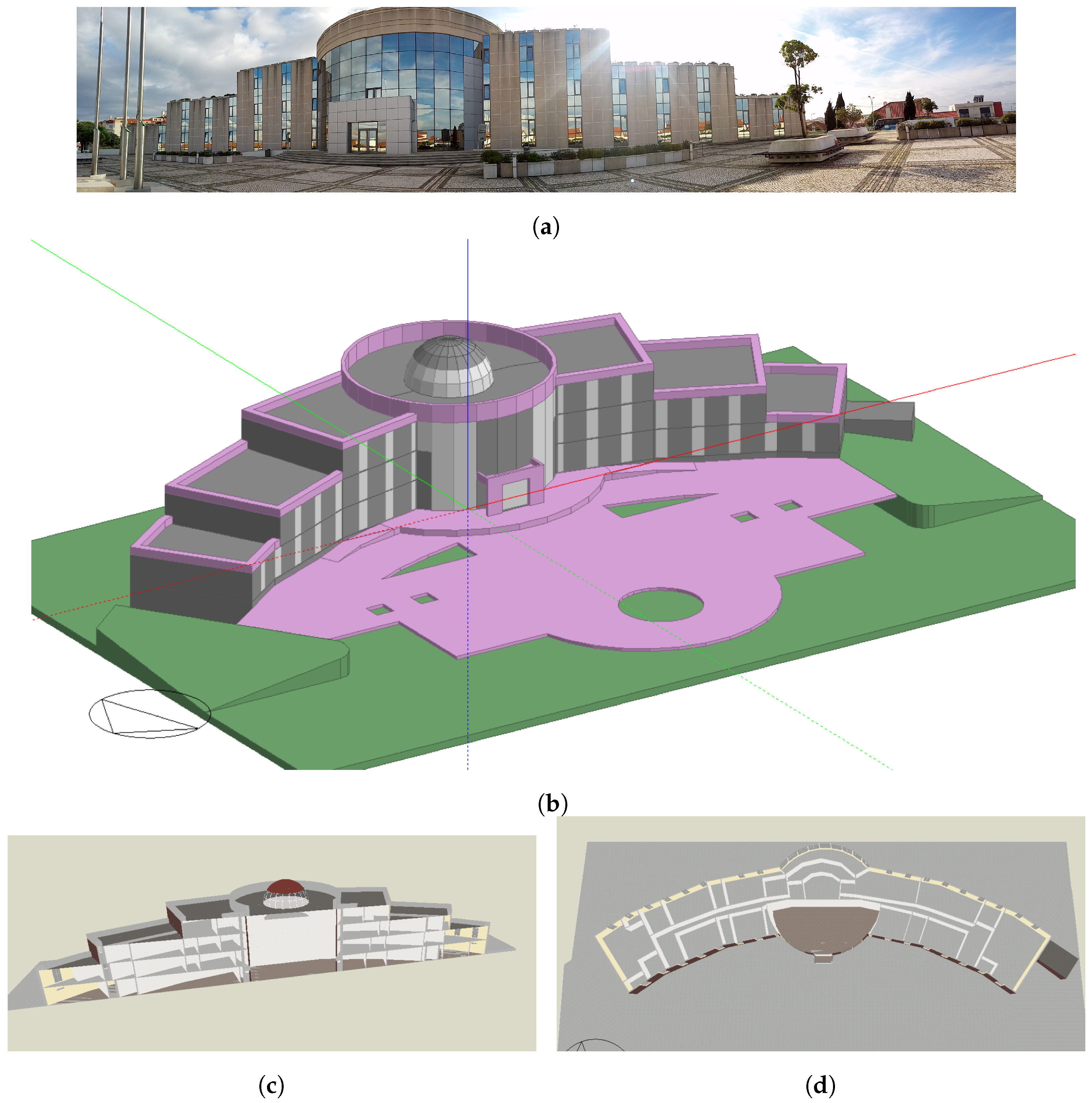
4.1. The Example Building

As a running example, one of the MOEEBIUS project buildings was used: the Mafra City Hall in the northwest of Lisbon District (Portugal) shown in Figure 5. It is a four stories building (three over ground and one semi-exposed basement), which sums around 4800${\mathrm{m}}^2$, with its main façade west oriented, with large openings and a central atrium. It houses about 200 permanent staff and about 50 visitors per day, including the mayor’s office and administrative spaces. Electricity is used as energy carrier to cover all buildings’ needs (more information about the specific building as well as the other MOEEBIUS Project buildings can be found in the project website: www.moeebius.eu).

A simulation model of the building was created using EnergyPlus. The architectural plans and material properties of walls and glazings were gathered from the municipality. The 3D geometrical modelling and the thermal properties definition (roof, floors/ceilings, external walls, internal walls, openings, etc.) were carried out using DesignBuilder (v4.7.0.027, Design-Builder Software Ltd., Gloucestershire, UK) [92], from which the first version of EnergyPlus Input Data File (IDF) was exported. The building is located on a top of a hill, so the surrounding ground was included in the model, but any effect of shading by neighbourhood constructions is neglectable. Once exported to EnergyPlus, the model was enriched with zone and activity modelling (activity schedules, occupancy densities, metabolic rates, equipment internal gains and thermal comfort and internal air quality setpoints) and the simulation time-step was set to 10-min intervals.

In the last step, the thermal/electrical loads and distributed generation systems existing in the building were introduced into the model. Here, as the HVAC system represents the main load of the building, special attention was paid to include a reliable model, reproducing the typology and topology of the building’s actual systems. The heating and cooling demand of the building is covered by 13 Variable Refrigerant Flow (VRF) centralised systems that can provide heating and cooling simultaneously according to the specific needs of each of the spaces of the building. Each of the VRF systems is formed by an external unit, connected to several internal units deployed at zone level that can provide independent temperature control to each of the conditioned rooms. Technically, a VRF system is an Air-Conditioning (AC) system, consisting of one external and several space-level terminal units, which operates by varying the refrigerant flow rate, using variable speed compressors (in the external units) and electronic expansion valves (in the space-level terminal units), to meet the heating and/or cooling demands of the building. The ventilation system of the building is formed by several independent supply and exhaust fans, connected respectively to supply and exhaust duct networks, enabling internal air renewal, however not providing exhaust air heat recovery functionality. All of them operate according to constant air volume control strategies. Concerning the Domestic Hot Water (DHW), small electrical domestic water heaters are installed in specific zones (e.g., cafe and restrooms), due to low DHW demands at these areas. Finally, the thermal/electrical loads related to indoor lighting, cafeteria appliances and offices/IT equipment were introduced into the model according to their specification data-sheets.

Occupant thermal comfort was evaluated using the Fanger predicted mean vote PMV index—following relevant standards [28]—which predicts the thermal sensation of a large group of people on a seven-point scale from too cold (−3) to too hot (+3). For the PMV estimation in our simulation model, constant values of metabolic rate (108$\mathrm{W}/\mathrm{person}$ corresponding to light-office activities), clothing level (0.5$\mathrm{clo}$) and in-space air velocity (0.137$\mathrm{m}/\mathrm{s}$) were considered. Note here that, instead of using the Fanger index, any personalised thermal comfort model [35,36,37,38,39] can be seamlessly integrated in the overall methodology; the only change will be in the thermal discomfort calculation methodology.

4.2. The Experimental Setup

As a proof-of-concept, we illustrate our methodology in simulation (i.e., we demonstrate only the upper part of Figure 2), by a one-day control design experiment using both the MCDA and GP_SS approaches. The simulation day was 1 (July 1st – a hot Summer day) and we utilised a Meteonorm weather file [93] for Lisbon, Portugal.

For our experiment, we focused on VRF5 control, which serves Rooms 21, 22, 87 and 88. Rooms 21 and 87 have seven occupants each and Rooms 22 and 88 have only one. The occupants were assumed to enter the building at 08:15 in the morning and exit at 17:15 in the afternoon. Our task was to minimise the total energy consumption measured at the VRF unit while maintaining comfortable interiors in all related rooms. We used an open-loop supervisory controller consisting of nine setpoint values to be applied on every occupied hour (08:00–17:00); all the necessary low-level control logic for the setpoint tracking were defined in the EnergyPlus model developed. Note that we did not use a different setpoint for each room but rather defined an HVAC zone where the controller of all rooms included is the same. This is a standard practice for control complexity reduction in buildings both in industry and in research applications (e.g., see [94,95,96] and the references therein).

We have to emphasise here that, even though the control setpoint was the same for all rooms, the thermal comfort evaluation of the generated control solution was performed in each controlled room separately. Following the relevant standards [28,29], we used the Fanger index for thermal comfort evaluation and required that the Fanger PMV value in each office is within $(-0.5,+0.5)$ in all time-steps. In each time-step t and for each room i, we defined the following comfort constraint:

$$\begin{array}{c}\hfill c_t^i=\left\{\begin{array}{cc}\hfill 0,& \mathrm{if}-0.5\le {\mathrm{PMV}}_t^i\le +0.5\hfill \\ \hfill 10\ast {({\mathrm{PMV}}_t^i+0.5)}^2,& \mathrm{if}{\mathrm{PMV}}_t^i<-0.5\hfill \\ \hfill 10\ast {({\mathrm{PMV}}_t^i-0.5)}^2,& \mathrm{if}{\mathrm{PMV}}_t^i>+0.5\hfill \end{array}\right.\end{array}$$

(11)

Summarising, in connection with the classical MPC setup (Equation (1)), we had the following setup:

• The building is controlled only during the occupancy period (08:00–17:00).
• The control actions are hourly setpoints, which are the same for the four control offices. Thus, the control time-step is one hour.
• The thermal comfort constraints are defined according to Fanger PMV index and are posed as illustrated in Equation (11).
• The (predicted) exogenous factors in our case are the weather conditions (provided by the weather file) and the occupancy patterns (which are assumed fixed and known in advance).
• Since we consider that the predictions for the disturbances are accurate, there is no need to re-design our control strategy at each control time-step (i.e., every hour), so for the work presented here we design the entire control strategy once for the entire day. Of course, in future application in the real building frequent control, (re-)design will be required to compensate for all unpredicted disturbances.
• The evolution of the system dynamics is provided by the EnergyPlus simulator; as described earlier we do not have access to the internal equations of the simulator but we can only observe the input-output relationship.
• The objective/cost function to be minimised is the total energy consumption measured at the VRF5 unit, which serves the four controllable offices.

To evaluate the quality and efficiency of the improved control strategies under the MCDA and GP_SS experiments, we defined a simple Rule-Based (RB) controller of the building, which maintained a constant setpoint for all offices throughout the day. This setpoint was defined at 24.5${}^{\circ }\mathrm{C}$, after a set of test simulations with different setpoints and consultation of the relevant thermal comfort standards [28]. The performance of the Rule-Based controller can be seen in Figure 6a.

4.3. The Software Framework

For the simulation study presented here, we defined a co-simulation setup. Both the MCDA and GP_SS approaches were implemented in Python and, in each iteration of the applied algorithm, a controller (i.e., the setpoint values in our case) was evaluated in the EnergyPlus simulation model. The control logic (i.e., applying the first control action at 08:00 and the subsequent setpoints every 1 h) was implemented in Matlab and in each simulation time-step a control action was communicated from Matlab to EnergyPlus. EnergyPlus simulated the building dynamics for the following time-step and the building states and weather conditions for this time-step were communicated back in Matlab. This process repeated until the end of the simulation period (one day for our experiment here) and the results were communicated back to the Control Optimisation algorithm for further processing. The coupling between Matlab and EnergyPlus was achieved using the Building Controls Virtual Test Bed (BCVTB) co-simulation software (v8.6, Lawrence Berkeley National Laboratory, Cyclotron Rd, Berkeley, CA, USA) [97]. For all the experiments, we used a MacBook Pro laptop, equipped with a 2.8$\mathrm{GHz}$ Intel Core i7 processor and 16$\mathrm{GB}$ of RAM and we did not use any form of parallel computation. For the GP_SS implementation, we used the GPy library [98] for the Gaussian Process definition and the Sequential Least Squares Programming (SLSQP) algorithm [99] of the pyOpt Python library [100] for the constrained optimisation setup.

4.4. Results

4.4.1. Approach Using Multi-Criteria Decision Analysis

For the MCDA approach, we ran 12 simulations where the controller was a static setpoint throughout the day, similar to the rule-based controller. Here, we tried all setpoint values from 21.5${}^{\circ }\mathrm{C}$ to 27${}^{\circ }\mathrm{C}$ and we incremented the setpoint by 0.5${}^{\circ }\mathrm{C}$ in each simulation. The results for each controller are shown in

Table 1. The evaluation of different control strategies in the simulation model. Here, the thermal comfort constrained violations are calculated using Equation (11) for the entire occupied period.

Strategy	Setpoint	Energy	Thermal Comfort				MCDA Results
Index	Value	Consumption	Constraint Violation				${\mathit{w}}_1=10$	${\mathit{w}}_1=0$	${\mathit{w}}_1=5$
	(${}^{\circ }\mathbf{C}$)	($\mathbf{kWh}$)	R21	R22	R87	R88	${\mathit{w}}_2=0$	${\mathit{w}}_2=10$	${\mathit{w}}_2=5$
1	21.5	163.1	0.3	0.9	0.5	11.8	12	8	10
2	22.0	157.9	0.1	0.5	0.1	4.9	11	7	9
3	22.5	152.5	0.0	0.1	0.0	0.8	10	6	8
4	23.0	146.9	0.0	0.0	0.0	0.0	9	5	7
5	23.5	137.3	0.0	0.0	0.0	0.0	8	4	6
6	24.0	122.2	0.0	0.0	0.0	0.0	7	9	5
7	24.5	107.5	0.0	0.0	0.0	0.0	6	3	4
8	25.0	93.5	0.0	0.0	0.0	0.0	5	10	3
9	25.5	79.8	0.0	0.0	0.01	0.0	4	2	11
10	26.0	67.5	0.1	0.2	1.0	0.0	3	1	2
11	26.5	57.7	2.1	2.7	4.9	0.0	2	11	1
12	27.0	48.9	6.6	8.1	11.3	0.1	1	12	12

.

To illustrate the behaviour and performance of the MCDA approach, we implemented a series of experiments with different weights in the criteria, with the criteria being the energy consumption and thermal comfort violations shown in Table 1. The weights can take numbers from 0 to 10, with 0 meaning that this criterion is not important and 10 meaning that it is quite important (note that the weights of all the criteria do not need to add to 10. We are not trying to achieve a relevant weighting). Note that we assigned the same weight in all thermal comfort violations, since it is rare in real world applications that we prefer comfort in one room over another. Thus, we represented the importance of energy savings with the value of $w_1$ and the importance of thermal comfort with the value of $w_2$. The different weighting configurations (shown in Table 1) are the following:

• Weights: $w_1=10$ and $w_2=0$.
  • Reasoning: This is a weighting combination that gives priority to the energy consumption.
  • Result: The ranking of the strategies from PROMETHEE II algorithm is as expected, since the algorithm prioritises the solutions taking into account only the energy consumption criterion.
• Weights: $w_1=0$ and $w_2=10$.
  • Reasoning: This is a weighting combination that gives priority to the thermal comfort conditions in the building.
  • Result: The algorithm favours solutions that maintain comfortable interiors, but the highest ranking controller is the one with the minimum consumption among all the controllers that achieve comfort. This is one of the properties of the algorithm: even though we indicated that the energy consumption has no priority for us, the fact that this criterion needs to be minimised too leads to this sorting.
    We have to note here that, even though Strategy #9 leads to limited discomfort, it is not among the high-ranking strategies. This is due to the high priority given to the comfort criterion, which results into treating the constraint violations as hard constraints.
• Weights: $w_1=5$ and $w_2=5$.
  • Reasoning: This is a weighting combination that gives equal priority to both criteria.
  • Result: Here, the comfort violations are treated as soft constraints and the ranking of strategies is quite balanced, but the highest ranking strategy determined by the algorithm (Strategy #10) leads to significant discomfort in Office 87.

Concluding, for a fair comparison both with the baseline controller and the GP_SS solution, we have selected Strategy #9 (i.e., setpoint at 25.5${}^{\circ }\mathrm{C}$, shown in Figure 6b) as the “best one”, which results in 25% savings compared to the rule-based controller.

4.4.2. Approach Using Gaussian Process State Space Models

Here, we ran 20 simulations with random control actions and used the collected data for the initial training of the GP Regression model. For the training, we defined the following input features and target values (see also Figure 4) at time t:

• Input Features:
  • ${\widehat{w}}_t^1$: Outdoor Air Temperature
  • ${\widehat{w}}_t^2$: Global Solar Radiation in the Horizontal plane
  • ${\widehat{x}}_t^{1-4}$: Indoor Air Temperature of the four controlled rooms
  • ${\widehat{x}}_t^{5-8}$: Indoor Relative Humidity of the four controlled rooms
  • ${\widehat{x}}_t^{9-12}$: Fanger PMV value of the four controlled rooms
  • ${\widehat{x}}_t^{13}$: Energy consumption of VRF5 in the time-interval $(t-1,t)$
  • $u_t$: the control setpoint
• Target values: all states at time-step $t+1$, i.e., ${\widehat{x}}_{t+1}^{1-13}$.

Note that, even though we refer to the GP approximation as “GP model”, we defined 13 GP regressors—one for each target variable. When the model is trained, we utilise it for defining and solving the constrained optimisation problem of Equation (9) offline. Once the optimisation process finishes, the new controller is evaluated in the simulation model, the GP training data are augmented with the outcome of the new iteration and the process is repeated.

The resulting controller after five simulation/optimisation steps is shown in Figure 6c. The entire process (20 initial simulations + 5 simulation and optimisation steps) requires 90 min in our hardware configuration and leads to 32.9% energy improvement compared to the baseline controller and 9.5% compared to the “best” MCDA controller (see

Table 2. Energy consumption of VRF5 under the different control approaches.

Energy Consumption RB (kWh)	Energy Consumption MCDA (kWh)	Energy Consumption GP_SS GPSS (kWh)
107.5	79.8	72.1

for the consumption values, by allowing a small amount of discomfort in Room 87 only (0.2 as an absolute value calculated using Equation (11)).

As can be seen in Figure 6, these increased savings are due to the initial performance of the baseline controller. Here, the setpoint applied (24.5${}^{\circ }\mathrm{C}$) maintains the Fanger PMV values close to zero, being “unaware" constrained relaxation for PMV ($-0.5,+0.5$). The GP_SS and MCDA approaches on the other hand are capable of exploiting the trade-off between energy consumption and thermal comfort and discover control strategies that maintain PMV values close to the high bound of the constraint, thus saving energy. Another interesting observation is that there is not much variability to the control setpoints of the best control solution designed by the GP_SS approach. This is because the cooling system is air-based and capable of covering the cooling demand, so there are no time-delay effects, as we see in buildings equipped with systems such as radiators [4,25] or Thermally Activated Building Slabs (TABS) [2,25]. This would imply that only for this HVAC system a more targeted setpoint/control parameter search for the MCDA approach could lead to the same results as the fully-fledged optimisation methodology followed in GP_SS approach. Alternatively, an optimisation problem with only one parameter (i.e., a constant setpoint for the entire day) could also lead to an improved control strategy compared to the baseline controller.

5. Conclusions

In the work presented here, we defined and evaluated a model-assisted control optimisation methodology in buildings that is able to overcome the modelling cost problem of traditional MPC methodologies by replacing the mathematical model required in MPC with a detailed thermal simulation model of the building. A central part of our methodology is the control improvement (or optimisation) module, facilitating two simulation-based control improvement methodologies: one based in multi-criteria decision analysis methods and the other based on state-space identification of dynamical systems using Gaussian process models and model-based reinforcement learning. We evaluated both methods in a simulation study utilising an existing building in Portugal and we verified that they can generate more efficient controllers compared to a baseline control strategy, utilising only a small number of simulation calls.

More specifically, as indicated by our experiments, the flexibility of the GP_SS methodology to define different control setpoints in each control time-step can lead to more efficient control strategies. Here, including the thermal comfort bounds as constraints in the optimisation problem allows the algorithm to discover a good trade-off between thermal comfort conditions and energy consumption. Of course, the discovered controller does not correspond to the global optimal solution, but still is more efficient compared to the baseline control strategy.

The main benefit of the MCDA approach on the other hand is its simplicity and its negligible computational overhead. Despite this, it is almost impossible to define a set of meaningful and comfort preserving control strategies a priori for all types of buildings and controlled systems—some kind of control improvement or fine-tuning will always be required. In addition, we have seen that the method is particularly sensitive to the selection of the criteria weighting; here, the decision maker might need to actively take part in the final control strategy selection (e.g., by manually selecting one of the top N control strategies and not necessarily the highest ranked one).

We have to acknowledge that, for large buildings with centralised HVAC systems, the proposed approach might not scale. In the work presented here, we controlled only one of the 13 VRF units of the building, which implies that, if an online control design solution were required, we would need to run 13 control optimisation processes in parallel—a configuration that increases the computing infrastructure requirements and thus the associated cost. In addition, in the case of buildings with centralised control systems, the number of controlled parameters would be significantly higher, which would lead to a much harder constrained optimisation problem that would necessitate a higher number of simulation calls.

Of course, one could address this problem by utilising various simulation speed-up/simplification techniques reported in the literature (e.g., see [94,95,96] and the references therein), but still in the general case the posed constrained optimisation problem might be too large for this method. Another option would be to formulate the problem as a Reinforcement Learning setup and take advantage of recent advances in deep reinforcement learning research [101,102,103] combined with simulation to reality control transfer approaches [104,105] to mitigate the computationally complex problem of control design in the off-line phase.

Finally, as an immediate next step, we plan to apply the proposed methodology in the same real building in Portugal within the MOEEBIUS H2020 European Project, in an effort to evaluate the effect inaccurate predictions and user actions potentially have in the efficiency of our methodology.

References

1. Roth, K.W.; Westphalen, D.; Feng, M.Y.; Llana, P.; Quartararo, L. Energy Impact of Commercial Building Controls and Performance Diagnostics: Market Characterization, Energy Impact of Building Faults And Energy Savings Potential; Final Report; TAIX LLC: Cambrige, MA, USA, 2005; p. 412. [Google Scholar]
2. Kontes, G.D. Model-Assisted Control for Energy Efficiency in Buildings. Ph.D. Thesis, School of Production Engineering and Management, Technical University of Crete, University Campus, Chania, Greece, 2017. [Google Scholar]
3. Oldewurtel, F.; Parisio, A.; Jones, C.N.; Gyalistras, D.; Gwerder, M.; Stauch, V.; Lehmann, B.; Morari, M. Use of model predictive control and weather forecasts for energy efficient building climate control. Energy Build. 2012, 45, 15–27. [Google Scholar] [CrossRef] [Green Version]
4. Kontes, G.D.; Valmaseda, C.; Giannakis, G.I.; Katsigarakis, K.I.; Rovas, D.V. Intelligent BEMS design using detailed thermal simulation models and surrogate-based stochastic optimization. J. Process Control 2014, 24, 846–855. [Google Scholar] [CrossRef]
5. Afram, A.; Janabi-Sharifi, F. Theory and applications of HVAC control systems–A review of model predictive control (MPC). Build. Environ. 2014, 72, 343–355. [Google Scholar] [CrossRef]
6. Sturzenegger, D.; Gyalistras, D.; Morari, M.; Smith, R.S. Model predictive climate control of a swiss office building: Implementation, results, and cost–benefit analysis. IEEE Trans. Control Syst. Technol. 2016, 24, 1–12. [Google Scholar] [CrossRef]
7. Liang, W.; Quinte, R.; Jia, X.; Sun, J.Q. MPC control for improving energy efficiency of a building air handler for multi-zone VAVs. Build. Environ. 2015, 92, 256–268. [Google Scholar] [CrossRef]
8. Mei, J.; Xia, X. Energy-efficient predictive control of indoor thermal comfort and air quality in a direct expansion air conditioning system. Appl. Energy 2017, 195, 439–452. [Google Scholar] [CrossRef]
9. Godina, R.; Rodrigues, E.M.; Pouresmaeil, E.; Catalão, J.P. Optimal residential model predictive control energy management performance with PV microgeneration. Comput. Oper. Res. 2018, 96, 143–156. [Google Scholar] [CrossRef]
10. Hilliard, T.; Swan, L.; Qin, Z. Experimental implementation of whole building MPC with zone based thermal comfort adjustments. Build. Environ. 2017, 125, 326–338. [Google Scholar] [CrossRef]
11. Ascione, F.; Bianco, N.; De Stasio, C.; Mauro, G.M.; Vanoli, G.P. A new comprehensive approach for cost-optimal building design integrated with the multi-objective model predictive control of HVAC systems. Sustain. Cities Soc. 2017, 31, 136–150. [Google Scholar] [CrossRef]
12. Razmara, M.; Maasoumy, M.; Shahbakhti, M.; Robinett, R., III. Optimal exergy control of building HVAC system. Appl. Energy 2015, 156, 555–565. [Google Scholar] [CrossRef]
13. Fiorentini, M.; Wall, J.; Ma, Z.; Braslavsky, J.H.; Cooper, P. Hybrid model predictive control of a residential HVAC system with on-site thermal energy generation and storage. Appl. Energy 2017, 187, 465–479. [Google Scholar] [CrossRef] [Green Version]
14. Godina, R.; Rodrigues, E.M.; Pouresmaeil, E.; Matias, J.C.; Catalão, J.P. Model predictive control home energy management and optimization strategy with demand response. Appl. Sci. 2018, 8, 408. [Google Scholar] [CrossRef]
15. Gwerder, M.; Tödtli, J.; Lehmann, B.; Dorer, V.; Güntensperger, W.; Renggli, F. Control of thermally activated building systems (TABS) in intermittent operation with pulse width modulation. Appl. Energy 2009, 86, 1606–1616. [Google Scholar] [CrossRef]
16. Tödtli, J.; Gwerder, M.; Lehmann, B.; Renggli, F.; Dorer, V. TABS-control: Steuerung und Regelung von thermoaktiven Bauteilsystemen. In Handbuch für Planung, Auslegung und Betrieb, Schriftenreihe Technik, Faktor-Verl, Zürich; FAKTOR Verlag AG: Zurich, Switzerland, 2009. [Google Scholar]
17. Moroşan, P.D.; Bourdais, R.; Dumur, D.; Buisson, J. Building temperature regulation using a distributed model predictive control. Energy Build. 2010, 42, 1445–1452. [Google Scholar] [CrossRef]
18. Cigler, J.; Prívara, S. Subspace identification and model predictive control for buildings. In Proceedings of the 2010 11th International Conference on Control Automation Robotics & Vision (ICARCV), Marina Bay Sands Resort, Singapore, 7–10 December 2010; pp. 750–755. [Google Scholar]
19. Širokỳ, J.; Oldewurtel, F.; Cigler, J.; Prívara, S. Experimental analysis of model predictive control for an energy efficient building heating system. Appl. Energy 2011, 88, 3079–3087. [Google Scholar] [CrossRef]
20. Nghiem, T.X.; Pappas, G.J. Receding-horizon supervisory control of green buildings. In Proceedings of the American Control Conference (ACC), San Francisco, CA, USA, June 29–July 1 2011; pp. 4416–4421. [Google Scholar]
21. Ma, Y.; Anderson, G.; Borrelli, F. A distributed predictive control approach to building temperature regulation. In Proceedings of the American Control Conference (ACC), San Francisco, CA, USA, June 29–July 1 2011; pp. 2089–2094. [Google Scholar]
22. Buderus, J.; Dentel, A. Generalization Approach for Models of Thermal Buffer Storages in Predictive Control Strategies. In Proceedings of the 15th IBPSA Conference, San Francisco, CA, USA, 7–9 August 2017. [Google Scholar]
23. Sturzenegger, D.; Gyalistras, D.; Semeraro, V.; Morari, M.; Smith, R.S. BRCM Matlab toolbox: Model generation for model predictive building control. In Proceedings of the American Control Conference (ACC), Portland, OR, USA, 4–6 June 2014; pp. 1063–1069. [Google Scholar]
24. Cauchi, N.; Abate, A. Benchmarks for cyber-physical systems: A modular model library for building automation systems (Extended version). arXiv, 2018; arXiv:1803.06315. [Google Scholar]
25. Kontes, G.D.; Giannakis, G.I.; Horn, P.; Steiger, S.; Rovas, D.V. Using thermostats for indoor climate control in office buildings: The effect on thermal comfort. Energies 2017, 10, 1368. [Google Scholar] [CrossRef]
26. Fisk, W.J. Health and productivity gains from better indoor environments and their relationship with building energy efficiency. Annu. Rev. Energy Environ. 2000, 25, 537–566. [Google Scholar] [CrossRef]
27. Akimoto, T.; Tanabe, S.i.; Yanai, T.; Sasaki, M. Thermal comfort and productivity-Evaluation of workplace environment in a task conditioned office. Build. Environ. 2010, 45, 45–50. [Google Scholar] [CrossRef]
28. International Organization for Standardization. ISO 7730:2005 -Ergonomics of the Thermal Environment: Analytical Determination and Interpretation of Thermal Comfort Using Calculation of the PMV and PPD Indices and Local Thermal Comfort Criteria; International Organization for Standardization: Geneva, Switzerland, 2005. [Google Scholar]
29. Standard, A. Standard 55-2013. In Thermal Environmental Conditions for Human Occupancy; ASHRAE: Atlanta, GA, USA, 2013; pp. 9–11. [Google Scholar]
30. Zavala, V.M. Real-time optimization strategies for building systems. Ind. Eng. Chem. Res. 2012, 52, 3137–3150. [Google Scholar] [CrossRef]
31. Klauco, M.; Kvasnica, M. Explicit MPC approach to PMV-based thermal comfort control. In Proceedings of the 53rd IEEE Conference on Decision and Control, Los Angeles, CA, USA, 15–17 December 2014; pp. 4856–4861. [Google Scholar]
32. Cigler, J.; Prívara, S.; Váňa, Z.; Žáčeková, E.; Ferkl, L. Optimization of predicted mean vote index within model predictive control framework: Computationally tractable solution. Energy Build. 2012, 52, 39–49. [Google Scholar] [CrossRef]
33. Mařík, K.; Rojíček, J.; Stluka, P.; Vass, J. Advanced HVAC control: Theory vs. reality. IFAC Proc. Vol. 2011, 44, 3108–3113. [Google Scholar] [CrossRef]
34. Chen, X.; Wang, Q.; Srebric, J. Model predictive control for indoor thermal comfort and energy optimization using occupant feedback. Energy Build. 2015, 102, 357–369. [Google Scholar] [CrossRef] [Green Version]
35. Lee, S.; Bilionis, I.; Karava, P.; Tzempelikos, A. A Bayesian approach for probabilistic classification and inference of occupant thermal preferences in office buildings. Build. Environ. 2017, 118, 323–343. [Google Scholar] [CrossRef]
36. Yan, D.; Hong, T.; Dong, B.; Mahdavi, A.; D’Oca, S.; Gaetani, I.; Feng, X. IEA EBC Annex 66: Definition and simulation of occupant behavior in buildings. Energy Build. 2017, 156, 258–270. [Google Scholar] [CrossRef] [Green Version]
37. Ghahramani, A.; Tang, C.; Becerik-Gerber, B. An online learning approach for quantifying personalized thermal comfort via adaptive stochastic modeling. Build. Environ. 2015, 92, 86–96. [Google Scholar] [CrossRef] [Green Version]
38. Malavazos, C.; Tsatsakis, K.; Tsitsanis, A. Towards a “context aware” flexibility profiling mechanism for the energy management environment. In Proceedings of the MedPower Conference, Athens, Greece, 2–5 November 2014; pp. 2–5. [Google Scholar]
39. Nagy, Z.; Yong, F.Y.; Schlueter, A. Occupant centered lighting control: a user study on balancing comfort, acceptance, and energy consumption. Energy Build. 2016, 126, 310–322. [Google Scholar] [CrossRef]
40. Crawley, D.B.; Lawrie, L.K.; Winkelmann, F.C.; Buhl, W.F.; Huang, Y.J.; Pedersen, C.O.; Strand, R.K.; Liesen, R.J.; Fisher, D.E.; Witte, M.J.; et al. EnergyPlus: creating a new-generation building energy simulation program. Energy Build. 2001, 33, 319–331. [Google Scholar] [CrossRef]
41. Wetter, M.; Zuo, W.; Nouidui, T.S.; Pang, X. Modelica buildings library. J. Build. Perform. Simul. 2014, 7, 253–270. [Google Scholar] [CrossRef]
42. Lilis, G.; Giannakis, G.; Kontes, G.; Rovas, D. Semi-automatic thermal simulation model generation from IFC data. In Proceedings of the European Conference on Product and Process Modelling, Vienna, Austria, 17 September 2014; pp. 503–510. [Google Scholar]
43. Bazjanac, V.; Maile, T.; O’Donnell, J.; Rose, C.; Mrazovic, N. Data environments and processing in semi-automated simulation with EnergyPlus. In Proceedings of the CIB W078-W102: 28th International Conference, Sophia Antipolis, France, 26–28 October 2011. [Google Scholar]
44. Lilis, G.N.; Giannakis, G.I.; Rovas, D.V. Automatic generation of second-level space boundary topology from IFC geometry inputs. Autom. Constr. 2017, 76, 108–124. [Google Scholar] [CrossRef] [Green Version]
45. Lilis, G.N.; Katsigarakis, K.; Giannakis, G.I.; Rovas, D. A cloud-based platform for IFC file enrichment with second-level space boundary topology. In Proceedings of the Joint Conference on Computing in Construction (JC3), Heraklion, Greece, 4–7 July 2017. [Google Scholar]
46. Andriamamonjy, A.; Saelens, D.; Klein, R. An automated IFC-based workflow for building energy performance simulation with Modelica. Autom. Constr. 2018, 91, 166–181. [Google Scholar] [CrossRef]
47. Lilis, G.N.; Giannakis, G.; Katsigarakis, K.; Rovas, D. District-aware Building Energy Performance simulation model generation from GIS and BIM data. In Proceedings of the BSO 2018: 4th Building Simulation and Optimization Conference, Cambridge, UK, 11–12 September 2018. [Google Scholar]
48. Giannakis, G. Development of Methodologies for Automatic Thermal Model Generation Using Building Information Models. Ph.D. Thesis, School of Production Engineering and Management, Technical University of Crete, University Campus, Chania, Greece, 2015. [Google Scholar]
49. Dean, S.; Mania, H.; Matni, N.; Recht, B.; Tu, S. On the sample complexity of the linear quadratic regulator. arXiv, 2017; arXiv:1710.01688. [Google Scholar]
50. Nghiem, T.X.; Jones, C.N. Data-driven demand response modeling and control of buildings with gaussian processes. In Proceedings of the American Control Conference (ACC), Seattle, WA, USA, 24–26 May 2017; pp. 2919–2924. [Google Scholar]
51. Jain, A.; Nghiem, T.; Morari, M.; Mangharam, R. Learning and control using Gaussian processes. In Proceedings of the 2018 ACM/IEEE 9th International Conference on Cyber-Physical Systems (ICCPS), Porto, Portugal, 11–13 April 2018; pp. 140–149. [Google Scholar]
52. Sutton, R.S.; Barto, A.G. Reinforcement Learning: An Introduction; MIT Press: Cambridge, MA, USA, 1998. [Google Scholar]
53. Deisenroth, M.P.; Fox, D.; Rasmussen, C.E. Gaussian processes for data-efficient learning in robotics and control. IEEE Trans. Pattern Anal. Mach. Intell. 2015, 37, 408–423. [Google Scholar] [CrossRef] [PubMed] [Green Version]
54. Bertsekas, D.P. Dynamic Programming and Optimal Control, 4th ed.; Approximate Dynamic Programming; Athena Scientific: Nashua, NH, USA, 2012; Volume II. [Google Scholar]
55. Prívara, S.; Váňa, Z.; Gyalistras, D.; Cigler, J.; Sagerschnig, C.; Morari, M.; Ferkl, L. Modeling and identification of a large multi-zone office building. In Proceedings of the 2011 IEEE International Conference on Control Applications (CCA), Denver, CO, USA, 28–30 September 2011; pp. 55–60. [Google Scholar]
56. Váňa, Z.; Kubeček, J.; Ferkl, L. Notes on finding black-box model of a large building. In Proceedings of the 2010 IEEE International Conference on Control Applications (CCA), Yokohama, Japan, 8–10 September 2010; pp. 1017–1022. [Google Scholar]
57. Garnier, A.; Eynard, J.; Caussanel, M.; Grieu, S. Low computational cost technique for predictive management of thermal comfort in non-residential buildings. J. Process Control 2014, 24, 750–762. [Google Scholar] [CrossRef]
58. Kolokotsa, D.; Pouliezos, A.; Stavrakakis, G.; Lazos, C. Predictive control techniques for energy and indoor environmental quality management in buildings. Build. Environ. 2009, 44, 1850–1863. [Google Scholar] [CrossRef]
59. Žáčeková, E.; Váňa, Z.; Cigler, J. Towards the real-life implementation of MPC for an office building: Identification issues. Appl. Energy 2014, 135, 53–62. [Google Scholar] [CrossRef]
60. Žáčeková, E.; Pcolka, M.; Sebek, M. On Satisfaction of the Persistent Excitation Condition for the Zone MPC: Numerical Approach. IFAC Proc. Vol. 2014, 47, 2848–2853. [Google Scholar] [CrossRef]
61. Van Overschee, P.; De Moor, B. Subspace iDentification for Linear Systems: Theory—Implementation—Applications; Springer Science & Business Media: Berlin, Germany, 2012. [Google Scholar]
62. Deisenroth, M.; Rasmussen, C.E. PILCO: A model-based and data-efficient approach to policy search. In Proceedings of the 28th International Conference on Machine Learning (ICML-11), Bellevue, WA, USA, 28 June 2011; pp. 465–472. [Google Scholar]
63. Schulman, J.; Levine, S.; Abbeel, P.; Jordan, M.; Moritz, P. Trust region policy optimization. In Proceedings of the International Conference on Machine Learning, Lille, France, 6–11 July 2015; pp. 1889–1897. [Google Scholar]
64. Recht, B. A Tour of Reinforcement Learning: The View from Continuous Control. arXiv, 2018; arXiv:1806.09460. [Google Scholar]
65. Schmidt, M.; Åhlund, C. Smart buildings as Cyber-Physical Systems: Data-driven predictive control strategies for energy efficiency. Renew. Sustain. Energy Rev. 2018, 90, 742–756. [Google Scholar] [CrossRef]
66. Eisenhower, B.; O’Neill, Z.; Narayanan, S.; Fonoberov, V.A.; Mezić, I. A methodology for meta-model based optimization in building energy models. Energy Build. 2012, 47, 292–301. [Google Scholar] [CrossRef]
67. Katsigarakis, K.; Kontes, G.; Giannakis, G.; Rovas, D. Sense-Think-Act Framework for Intelligent Building Energy Management. Comput.-Aided Civ. Infrastruct. Eng. 2016, 31, 50–64. [Google Scholar] [CrossRef]
68. Glaessgen, E.; Stargel, D. The digital twin paradigm for future NASA and US Air Force vehicles. In Proceedings of the 53rd AIAA/ASME/ASCE/AHS/ASC Structures, Structural Dynamics and Materials Conference 20th AIAA/ASME/AHS Adaptive Structures Conference 14th AIAA, Honolulu, HI, USA, 23–26 April 2012; p. 1818. [Google Scholar]
69. Coffey, B.; Haghighat, F.; Morofsky, E.; Kutrowski, E. A software framework for model predictive control with GenOpt. Energy Build. 2010, 42, 1084–1092. [Google Scholar] [CrossRef]
70. Henze, G.P.; Kalz, D.E.; Liu, S.; Felsmann, C. Experimental analysis of model-based predictive optimal control for active and passive building thermal storage inventory. HVAC R Res. 2005, 11, 189–213. [Google Scholar] [CrossRef]
71. Baldi, S.; Michailidis, I.; Kosmatopoulos, E.B.; Ioannou, P.A. A “plug and play” computationally efficient approach for control design of large-scale nonlinear systems using cosimulation: A combination of two “ingredients”. IEEE Control Syst. Mag. 2014, 34, 56–71. [Google Scholar]
72. Korkas, C.D.; Baldi, S.; Michailidis, I.; Kosmatopoulos, E.B. Intelligent energy and thermal comfort management in grid-connected microgrids with heterogeneous occupancy schedule. Appl. Energy 2015, 149, 194–203. [Google Scholar] [CrossRef]
73. Karagevrekis, A.; Baldi, S.; Michailidis, I.; Kosmatopoulos, E.B. Interconnected microgrids: An energyplus simulation test case. Mach. Rev. 2014, 1, 7–13. [Google Scholar]
74. Pichler, M.F.; Dröscher, A.; Schranzhofer, H.; Kontes, G.; Giannakis, G.; Kosmatopoulos, E.B.; Rovas, D. Simulation-assisted building energy performance improvement using sensible control decisions. In Proceedings of the Third ACM Workshop on Embedded Sensing Systems for Energy-Efficiency in Buildings, Seattle, WA, USA, 1–4 November 2011; pp. 61–66. [Google Scholar]
75. Olesen, B. International standards for the indoor environment. Indoor Air 2004, 14, 18–26. [Google Scholar] [CrossRef] [PubMed]
76. Luenberger, D.G.; Ye, Y. Linear and Nonlinear Programming; Springer: Berlin, Germany, 1984; Volume 2. [Google Scholar]
77. Calandra, R.; Gopalan, N.; Seyfarth, A.; Peters, J.; Deisenroth, M.P. Bayesian gait optimization for bipedal locomotion. In Proceedings of the International Conference on Learning and Intelligent Optimization, Gainesville, FL, USA, 16–21 February 2014; pp. 274–290. [Google Scholar]
78. Balaji, B.; Weibel, N.; Agarwal, Y. Managing Commercial HVAC Systems: What do Building Operators Really Need? arXiv, 2016; arXiv:1612.06025. [Google Scholar]
79. Diakaki, C.; Panagiotidou, N.; Pouliezos, A.; Kontes, G.D.; Stavrakakis, G.S.; Belibassakis, K.; Gerostathis, T.P.; Livanos, G.; Pagonis, D.N.; Theotokatos, G. A decision support system for the development of voyage and maintenance plans for ships. Int. J. Decis. Support Syst. 2015, 1, 42–71. [Google Scholar] [CrossRef]
80. Greco, S.; Figueira, J.; Ehrgott, M. Multiple Criteria Decision Analysis; Springer: Berlin, Germany, 2016. [Google Scholar]
81. Brans, J.P.; Mareschal, B. PROMETHEE methods. In Multiple Criteria Decision Analysis: State of the Art Surveys; Springer: Berlin, Germany, 2005; pp. 163–186. [Google Scholar]
82. Moffett, A.; Sarkar, S. Incorporating multiple criteria into the design of conservation area networks: A minireview with recommendations. Divers. Distrib. 2006, 12, 125–137. [Google Scholar] [CrossRef]
83. Mateo, J.R.S.C. Multi Criteria Analysis in the Renewable Energy Industry; Springer Science & Business Media: Berlin, Germany, 2012. [Google Scholar]
84. Kocijan, J.; Girard, A.; Banko, B.; Murray-Smith, R. Dynamic systems identification with Gaussian processes. Math. Comput. Model. Dyn. Syst. 2005, 11, 411–424. [Google Scholar] [CrossRef]
85. Rasmussen, C.E.; Williams, C.K. Gaussian Processes for Machine Learning; The MIT Press: Cambridge, MA, USA, 2006; Volume 38, pp. 715–719. [Google Scholar]
86. Schölkopf, B.; Smola, A.J.; Bach, F. Learning With Kernels: Support Vector Machines, Regularization, Optimization, and Beyond; MIT Press: Cambridge, MA, USA, 2002. [Google Scholar]
87. Brochu, E.; Cora, V.M.; De Freitas, N. A tutorial on Bayesian optimization of expensive cost functions, with application to active user modeling and hierarchical reinforcement learning. arXiv, 2010; arXiv:1012.2599. [Google Scholar]
88. Duvenaud, D.; Lloyd, J.R.; Grosse, R.; Tenenbaum, J.B.; Ghahramani, Z. Structure discovery in nonparametric regression through compositional kernel search. arXiv, 2013; arXiv:1302.4922. [Google Scholar]
89. May-Ostendorp, P.; Henze, G.P.; Corbin, C.D.; Rajagopalan, B.; Felsmann, C. Model-predictive control of mixed-mode buildings with rule extraction. Build. Environ. 2011, 46, 428–437. [Google Scholar] [CrossRef]
90. Domahidi, A.; Ullmann, F.; Morari, M.; Jones, C.N. Learning decision rules for energy efficient building control. J. Process Control 2014, 24, 763–772. [Google Scholar] [CrossRef]
91. Le, K.; Bourdais, R.; Guéguen, H. From hybrid model predictive control to logical control for shading system: A support vector machine approach. Energy Build. 2014, 84, 352–359. [Google Scholar] [CrossRef]
92. Tindale, A. Designbuilder Software; Design-Builder Software Ltd.: Gloucestershire, UK, 2005. [Google Scholar]
93. Remund, J.; Kunz, S. METEONORM: Global Meteorological Database for Solar Energy And Applied Climatology; Meteotest: Bern, Switzerland, 1997. [Google Scholar]
94. Giannakis, G.; Pichler, M.; Kontes, G.; Schranzhofer, H.; Rovas, D. Simulation speedup techniques for computationally demanding tasks. In Proceedings of the BS 2013: 13th Conference of the International Building Performance Simulation Association, Chambery, France, 26–28 August 2013; pp. 3761–3768. [Google Scholar]
95. Georgescu, M.; Mezić, I. Building energy modeling: A systematic approach to zoning and model reduction using Koopman Mode Analysis. Energy Build. 2015, 86, 794–802. [Google Scholar] [CrossRef]
96. Giannakis, G.; Kontes, G.; Korolija, I.; Rovas, D. Simulation-time Reduction Techniques for a Retrofit Planning Tool. In Proceedings of the BS 2017: 15th Conference of the International Building Performance Simulation Association, San Francisco, CA, USA, 7–9 August 2017; pp. 2014–2023. [Google Scholar]
97. Wetter, M. Co-simulation of building energy and control systems with the Building Controls Virtual Test Bed. J. Build. Perform. Simul. 2011, 4, 185–203. [Google Scholar] [CrossRef] [Green Version]
98. GPy. GPy: A Gaussian Process Framework in Python. 2012. Available online: http://github.com/SheffieldML/GPy (accessed on 27 November 2018).
99. Kraft, D. A software package for sequential quadratic programming. In Forschungsbericht- Deutsche Forschungs- und Versuchsanstalt fur Luft- und Raumfahrt; DFVLR: Braunschweig, Köln, 1988. [Google Scholar]
100. Perez, R.E.; Jansen, P.W.; Martins, J.R. pyOpt: A Python-based object-oriented framework for nonlinear constrained optimization. Struct. Multidiscip. Optim. 2012, 45, 101–118. [Google Scholar] [CrossRef]
101. Zhang, T.; Kahn, G.; Levine, S.; Abbeel, P. Learning deep control policies for autonomous aerial vehicles with mpc-guided policy search. arXiv, 2015; arXiv:1509.06791. [Google Scholar]
102. Mnih, V.; Kavukcuoglu, K.; Silver, D.; Rusu, A.A.; Veness, J.; Bellemare, M.G.; Graves, A.; Riedmiller, M.; Fidjeland, A.K.; Ostrovski, G.; et al. Human-level control through deep reinforcement learning. Nature 2015, 518, 529. [Google Scholar] [CrossRef] [PubMed]
103. Silver, D.; Huang, A.; Maddison, C.J.; Guez, A.; Sifre, L.; Van Den Driessche, G.; Schrittwieser, J.; Antonoglou, I.; Panneershelvam, V.; Lanctot, M.; et al. Mastering the game of Go with deep neural networks and tree search. Nature 2016, 529, 484. [Google Scholar] [CrossRef] [PubMed]
104. Rusu, A.A.; Vecerik, M.; Rothörl, T.; Heess, N.; Pascanu, R.; Hadsell, R. Sim-to-real robot learning from pixels with progressive nets. arXiv, 2016; arXiv:1610.04286. [Google Scholar]
105. Tobin, J.; Fong, R.; Ray, A.; Schneider, J.; Zaremba, W.; Abbeel, P. Domain randomization for transferring deep neural networks from simulation to the real world. In Proceedings of the 2017 IEEE/RSJ International Conference on Intelligent Robots and Systems (IROS), San Francisco, CA, USA, 7–9 August 2017; pp. 23–30. [Google Scholar]
Figure 1. The model predictive control paradigm for building control optimisation (adapted from [2,3]).
Energies 11 03376 g001
Figure 2. The simulation-based control improvement methodology.
Energies 11 03376 g002
Figure 3. Overview of simulation-based evaluation of building control strategies using multi-criteria decision analysis methods.
Energies 11 03376 g003
Figure 4. An off-line trajectory rollout using the identified GP state-space model.
Energies 11 03376 g004
Figure 5. The Mafra City Hall Building: (a) front view of the Mafra City Hall Building; (b) simulation of Mafra City Hall Building using DesignBuilder Software [92]; (c) the Mafra City Hall Building cut-off; and (d) the Mafra City Hall Building floor-plan.
Energies 11 03376 g005
Figure 6. The experimental results for the controlled/occupied period within one simulation day: (a) the performance of the simple rule-based controller with the setpoint 24.5 C ; (b) he performance of the best controller ranked by the MCDA method with the setpoint 25.5 C ; and (c) the performance of the optimised controller discovered by the GP_SS method with the setpoint varying per timestep, attaining values between 25.4 C and 26.1 C .
Energies 11 03376 g006