Experimental and Numerical Investigation of a MILD Combustion Chamber for Micro Gas Turbine Applications


Abstract
:1. Introduction
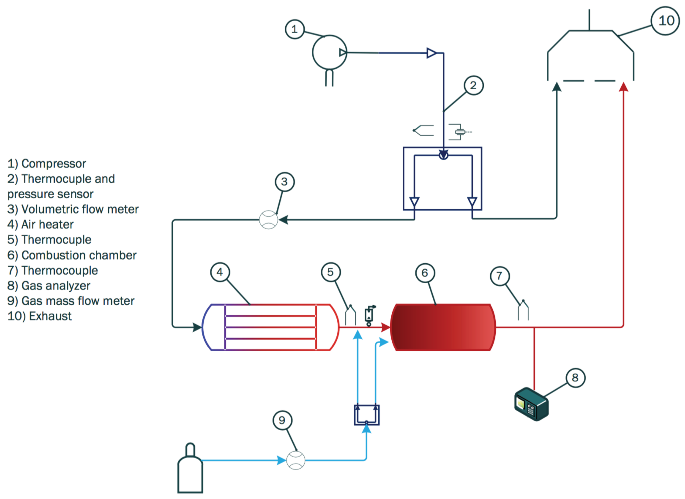
2. Experimental Setup
3. Experimental Results
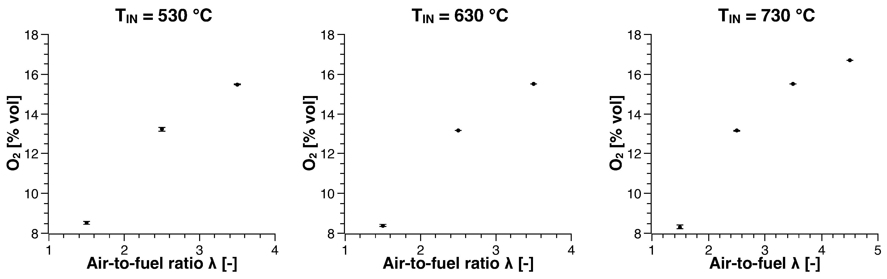
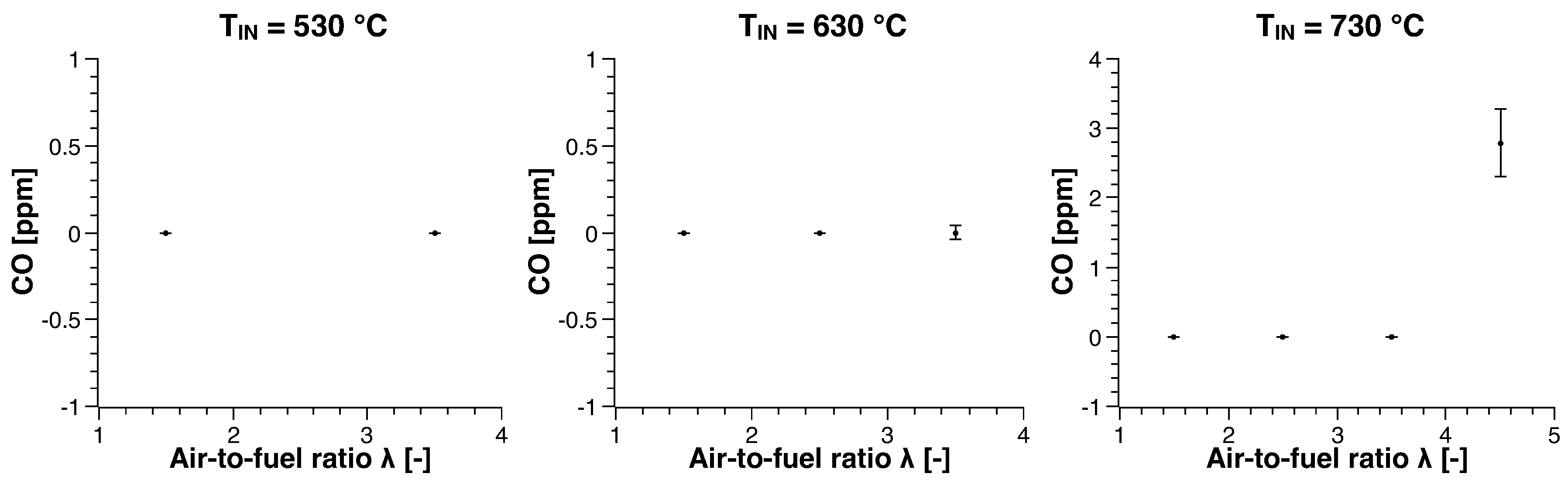
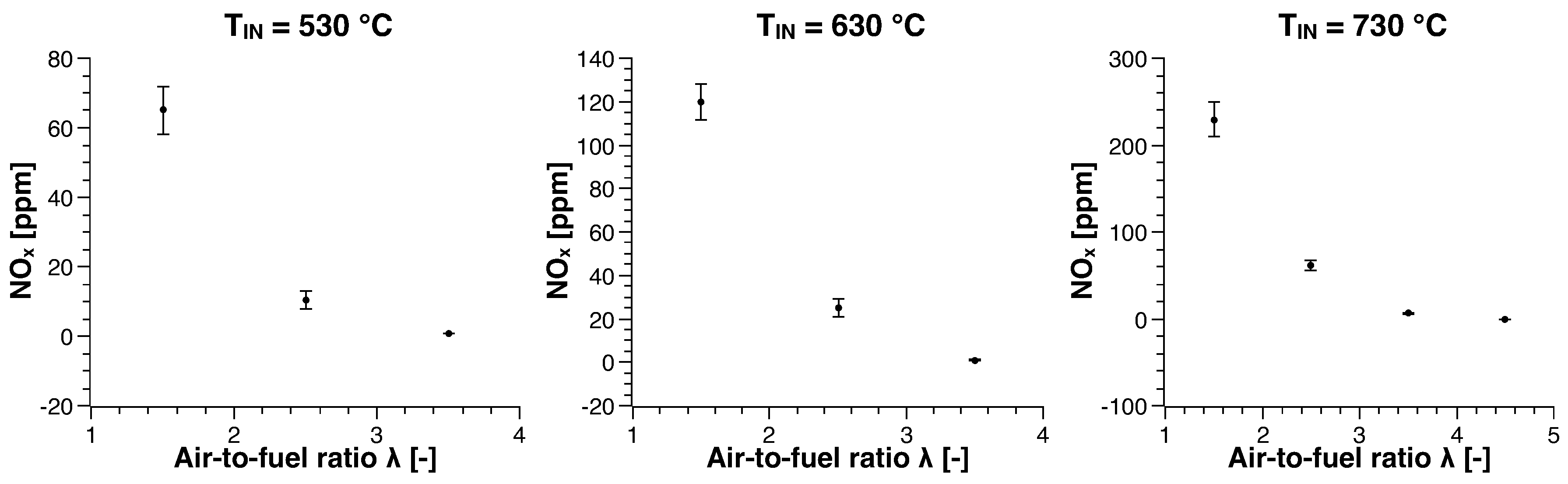
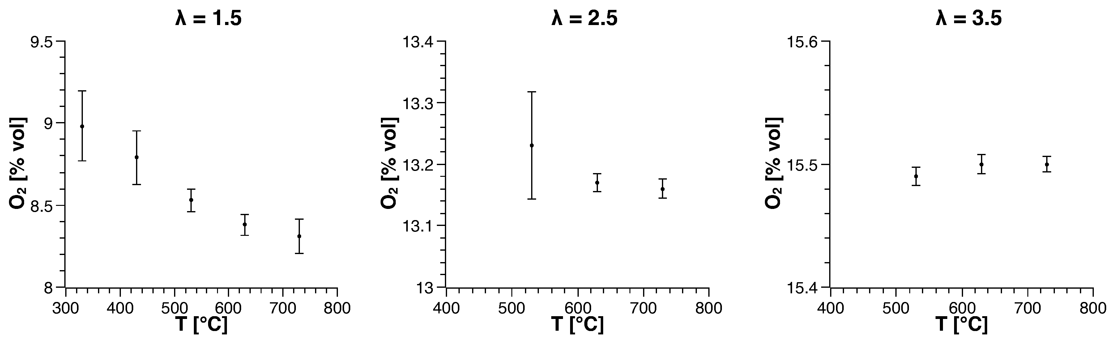
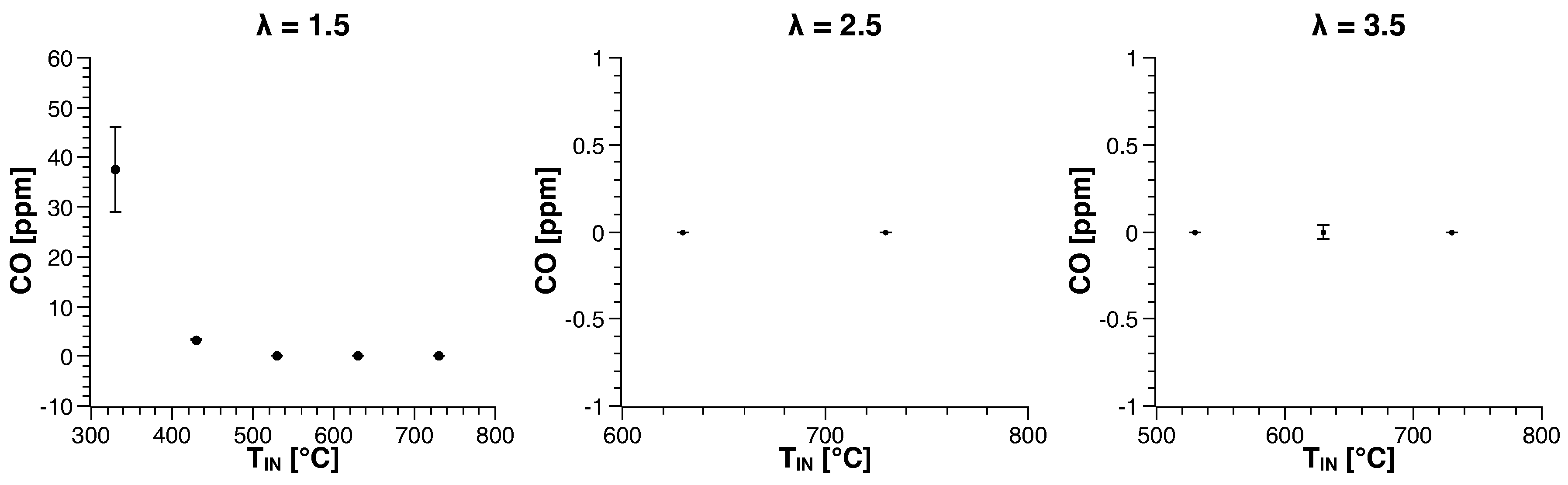
3.1. Methane
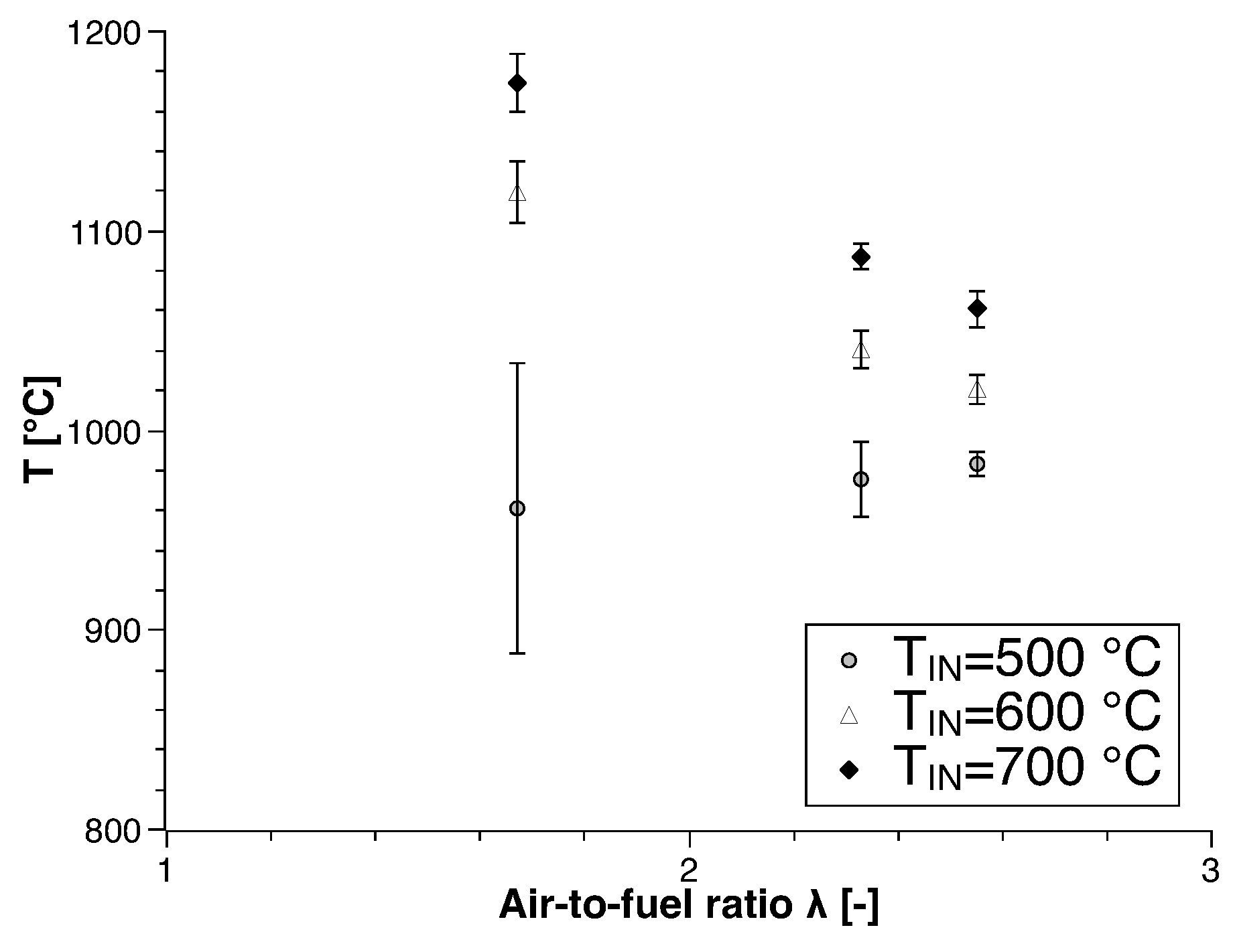
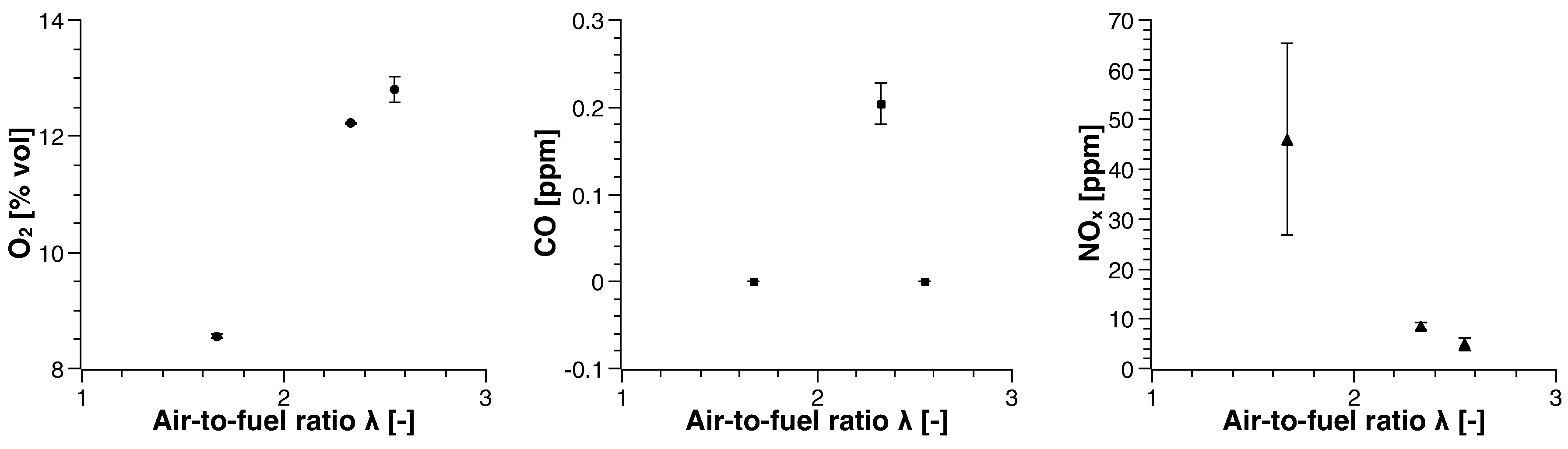
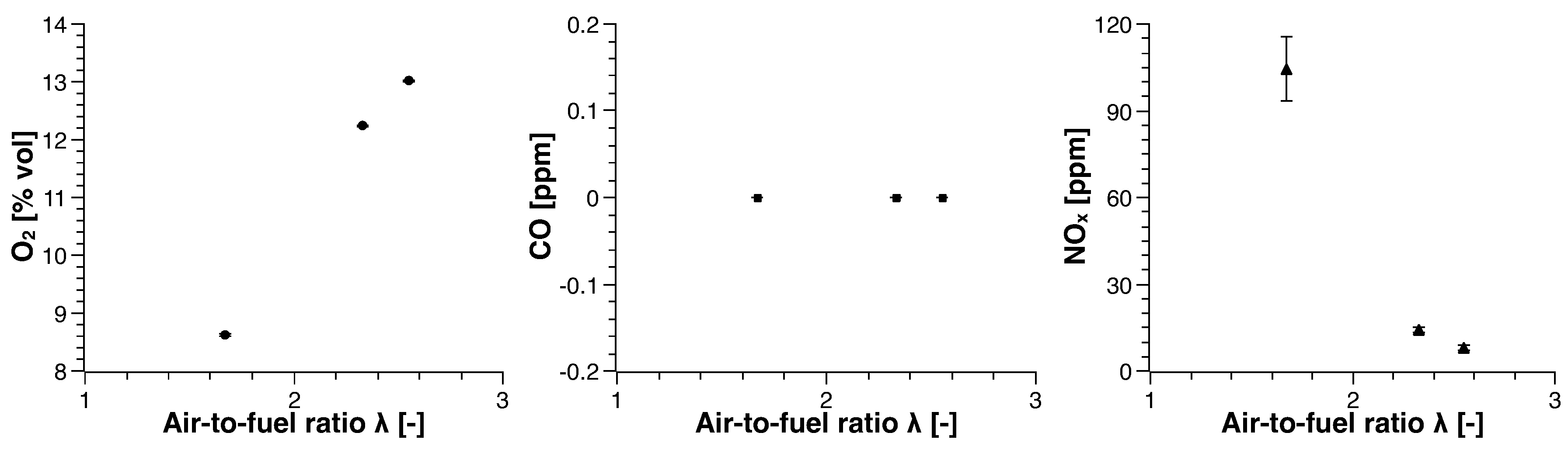
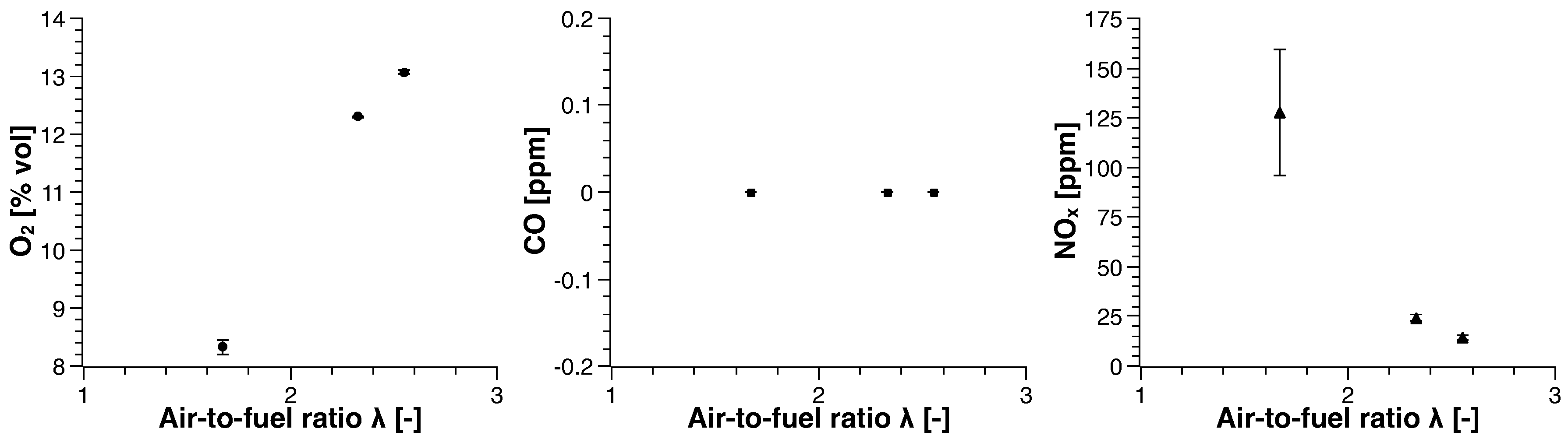
3.2. Biogas
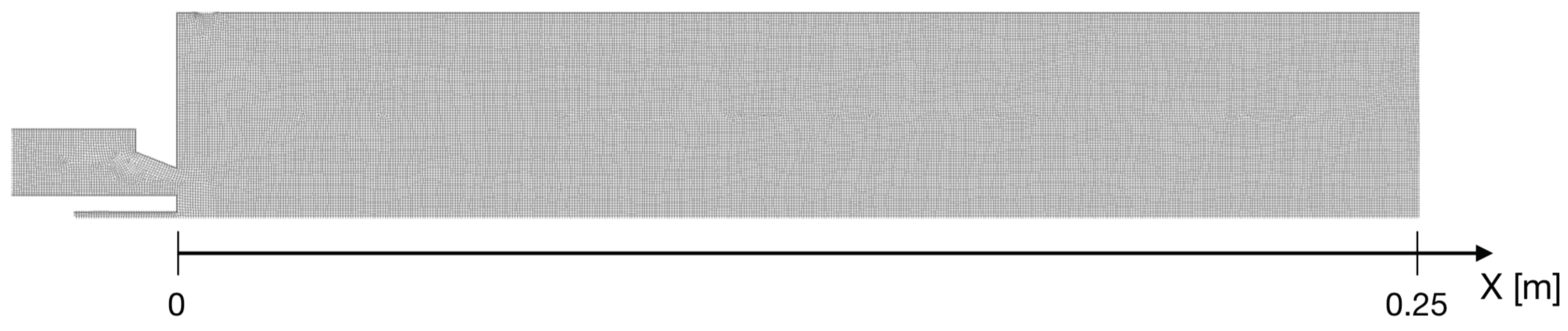
4. Numerical Study
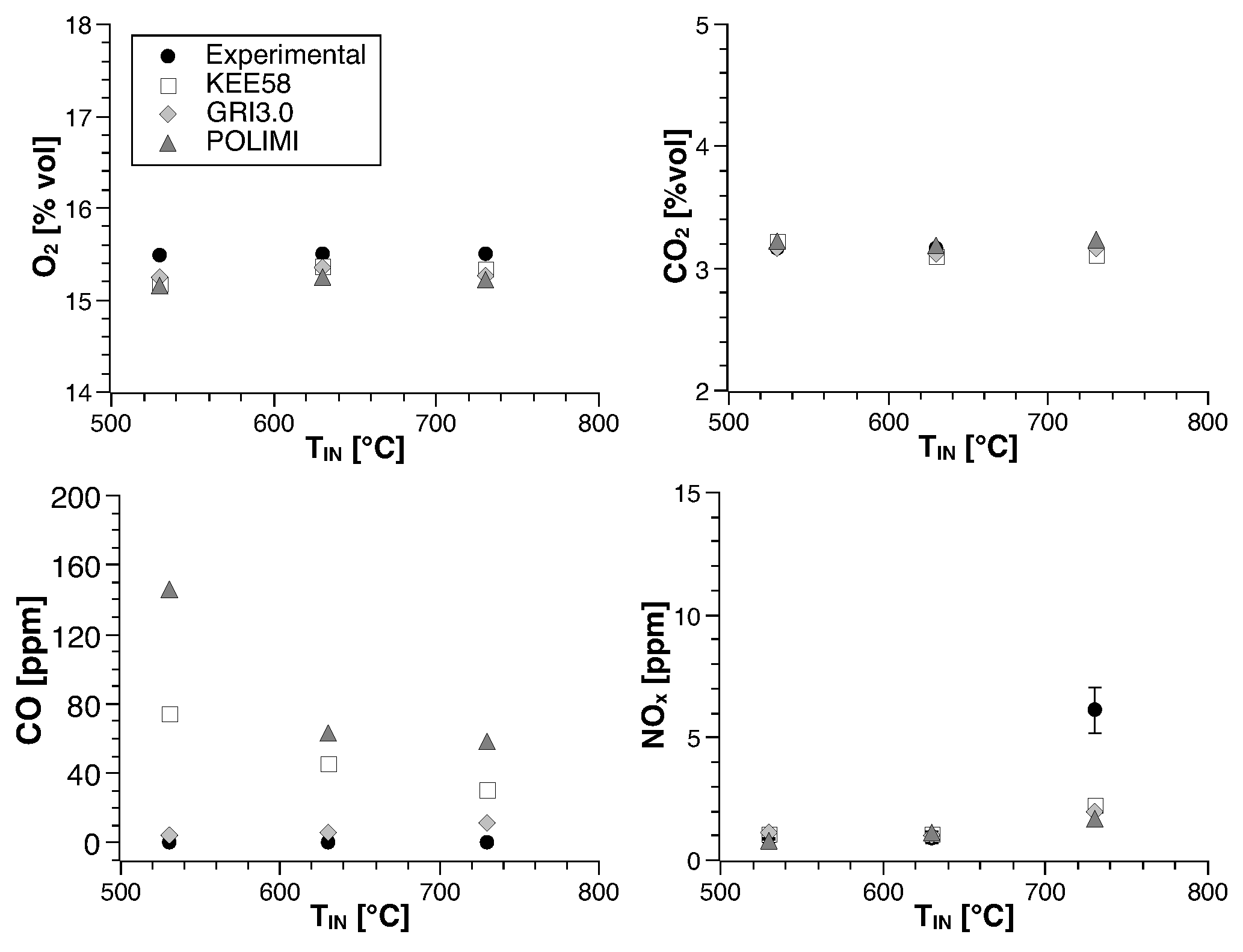
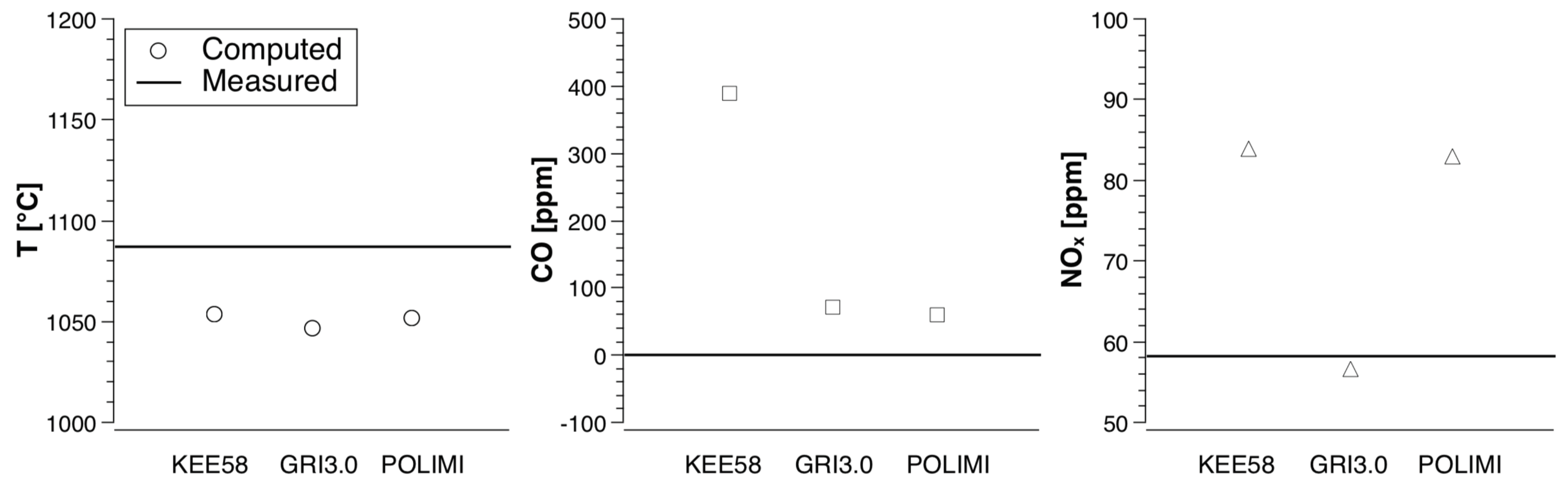
- KEE58 [42]; it consists of 17 species and 58 reversible chemical reactions.
- GRI 3.0 [43]; it is implemented without the NO reactions, resulting in 35 species and 217 reactions.
- POLIMI, a skeletal mechanism reduced ad hoc for the conditions of this combustion chamber. The reduction technique is based on a species-targeted sensitivity analysis, as explained by Stagni et al. [44]; it is obtained starting from the detailed mechanism POLIMI [45]. For methane, it consists of 25 species and 154 reactions, whereas for biogas 25 species and 170 reactions are needed.
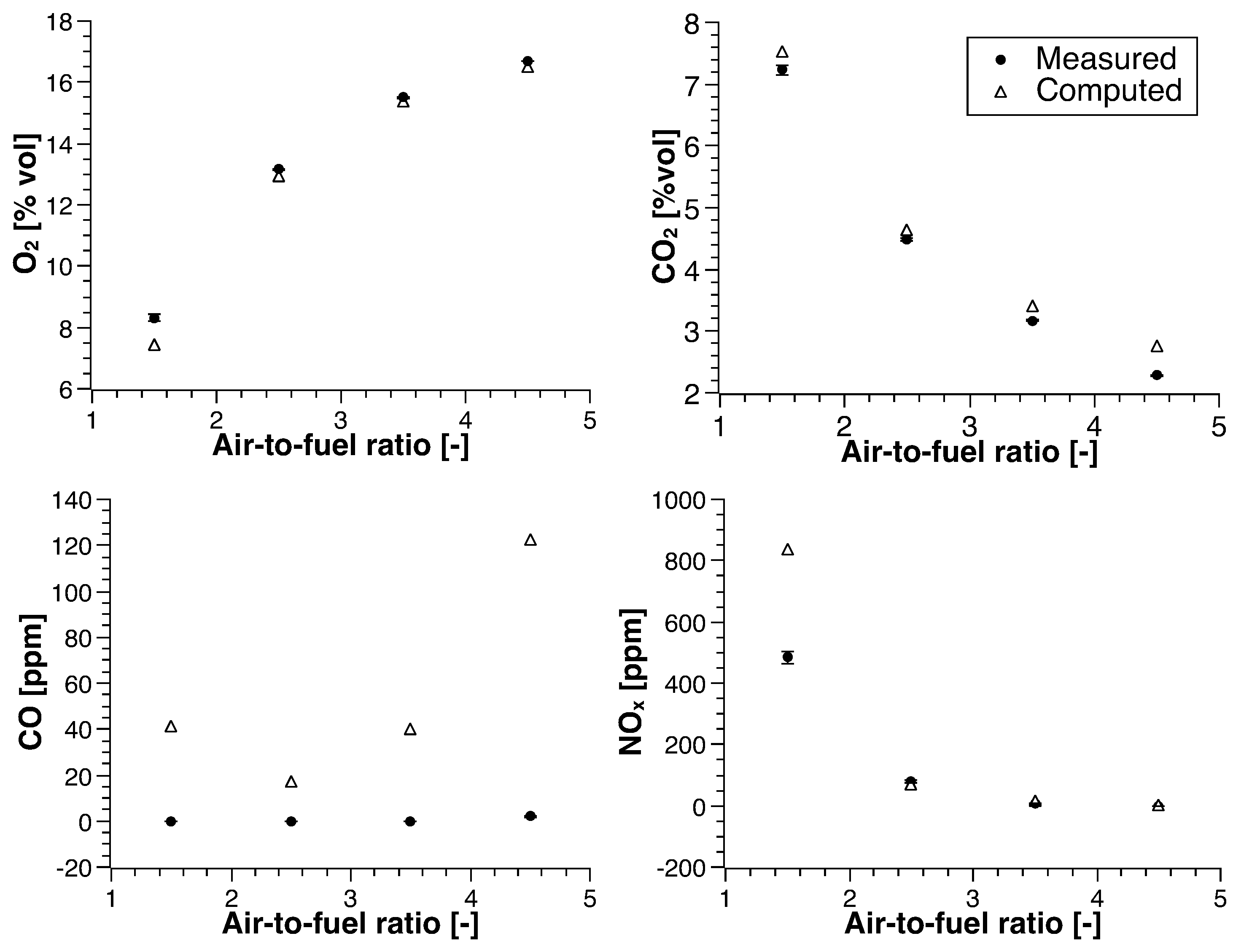
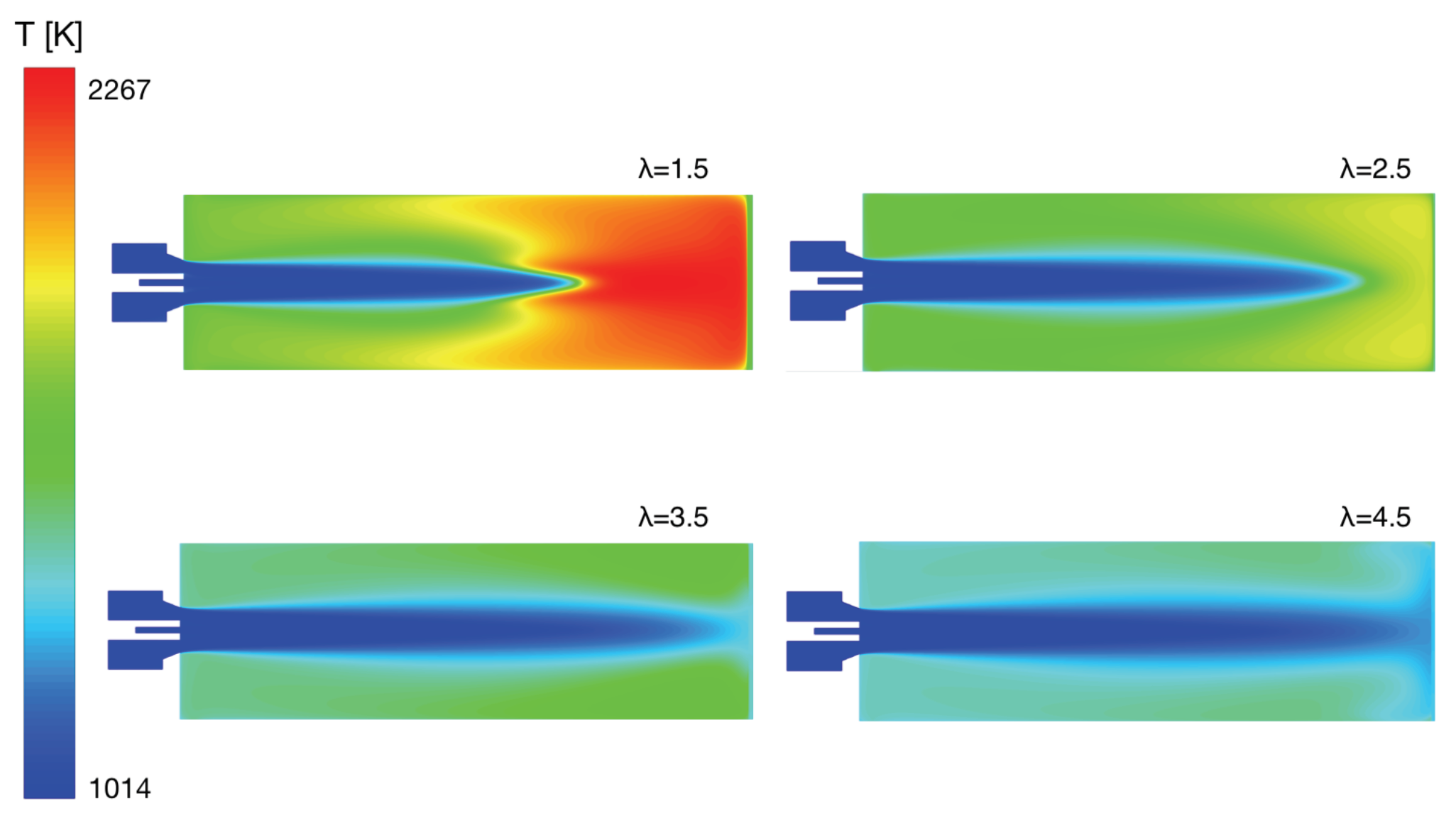
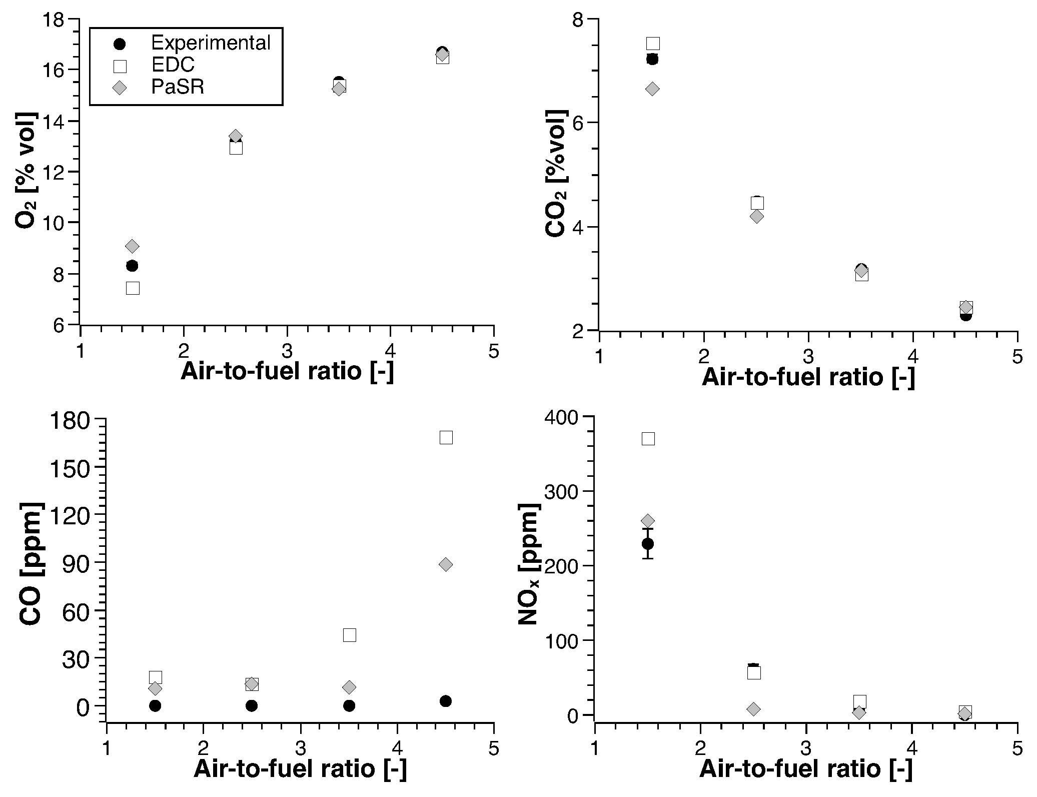
4.1. Methane
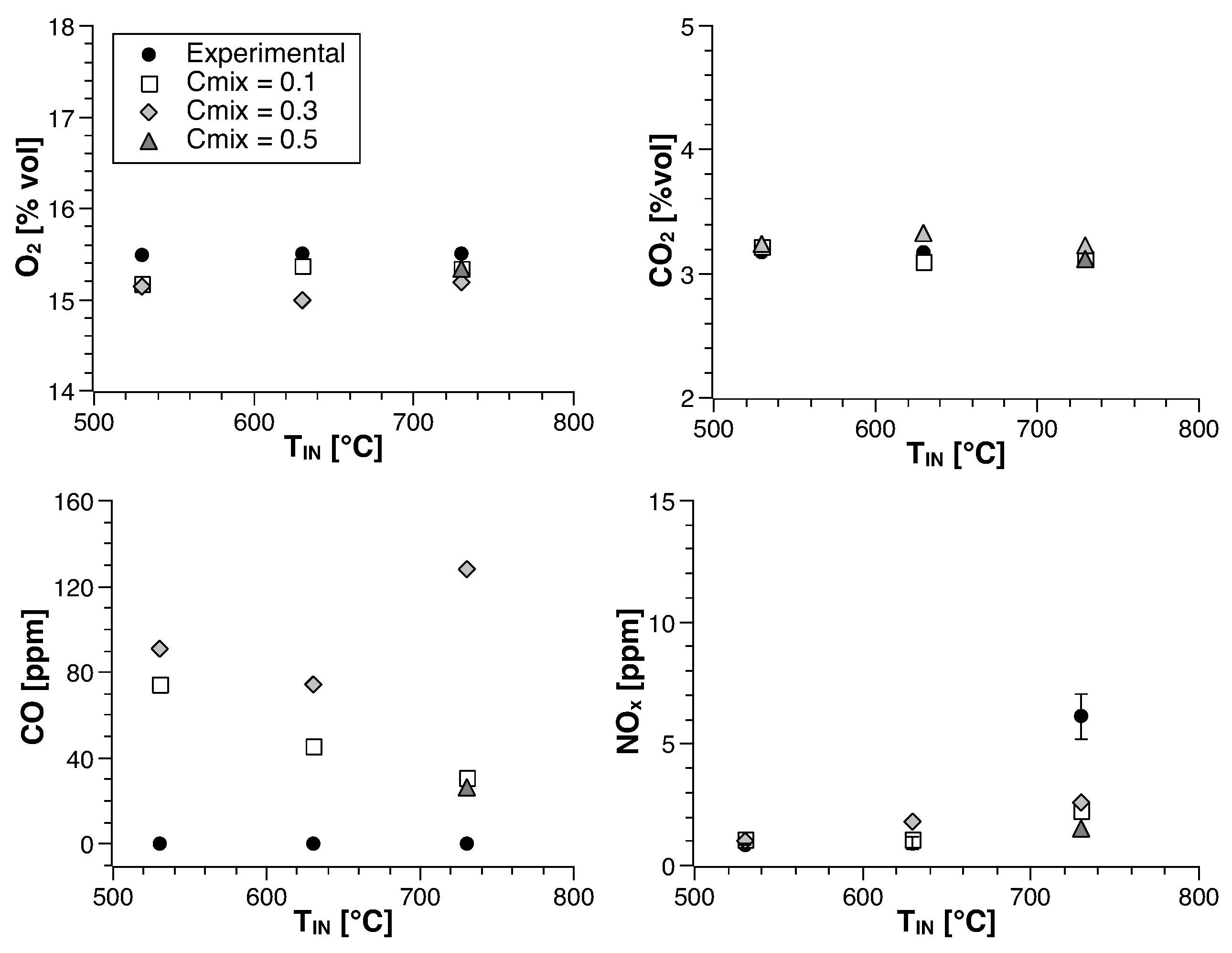
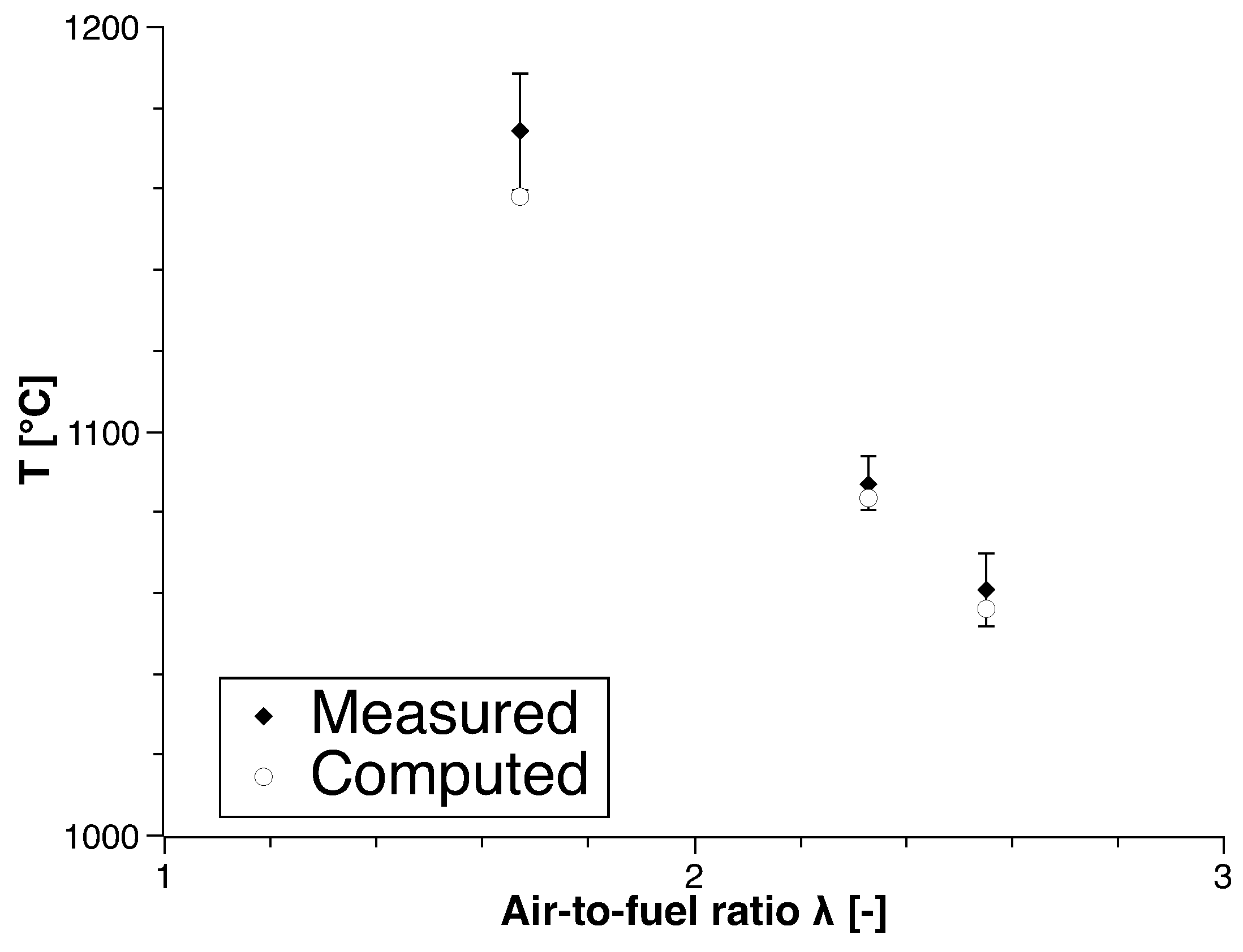
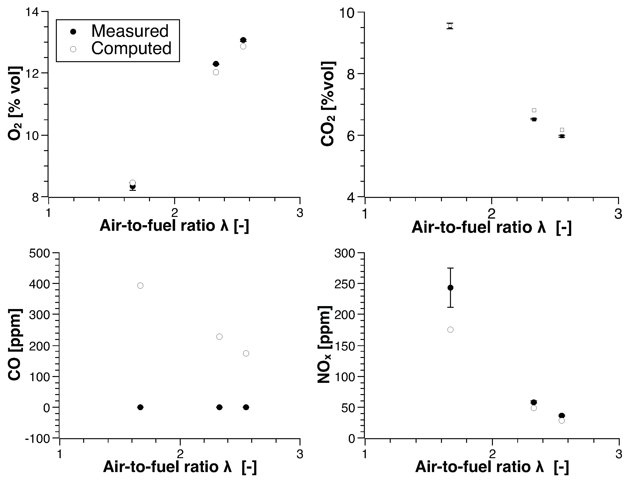
4.2. Biogas
5. Conclusions
Author Contributions
Conflicts of Interest
Abbreviations
| CFD | Computational Fluid Dynamic |
| EDC | Eddy Dissipation Concept |
| HiTAC | High Temperature Air Combustion |
| JHC | Jet in Hot Coflow |
| MILD | Moderate and Intense Low-Oxygen |
| mGT | Micro Gas Turbine |
| PaSR | Partially Stirred Reactor |
| Probability Density Function | |
| TPDF | Transorted Probability Density Function |
| UDF | User Defined Function |
References
- Onovwiona, H.; Ugursal, V. Residential cogeneration systems: review of the current technology. Renew. Sustain. Energy Rev. 2006, 10, 389–431. [Google Scholar] [CrossRef]
- Abagnale, C.; Cameretti, M.; De Robbio, R.; Tuccillo, R. Thermal Cycle and Combustion Analysis of a Solar-Assisted Micro Gas Turbine. Energies 2017, 10, 773. [Google Scholar] [CrossRef]
- Khidr, K.; Eldrainy, Y.; EL-Kassaby, M. Towards lower gas turbine emissions: Flameless distributed combustion. Renew. Sustain. Energy Rev. 2017, 67, 1237–1266. [Google Scholar] [CrossRef]
- Cavaliere, A.; de Joannon, M. Mild combustion. Prog. Energy Combust. Sci. 2004, 30, 329–366. [Google Scholar] [CrossRef]
- Wünning, J.; Wünning, J. Flameless oxidation to reduce thermal NO-formation. Prog. Energy Combust. Sci. 1997, 23, 81–94. [Google Scholar] [CrossRef]
- Gupta, A. Thermal characteristics of gaseous fuel flames using high temperature air. J. Eng. Gas Turbines Power 2004, 126, 9–19. [Google Scholar] [CrossRef]
- Kumar, S.; Paul, P.; Mukunda, H. Studies on a new high-intensity low-emission burner. Proc. Combust. Inst. 2002, 29, 1131–1137. [Google Scholar] [CrossRef] [Green Version]
- Dally, B.; Riesmeier, E.; Peters, N. Effect of fuel mixture on moderate and intense low oxygen dilution combustion. Combust. Flame 2004, 137, 418–431. [Google Scholar] [CrossRef]
- Duwig, C.; Stankovic, D.; Fuchs, L.; Li, G.; Gutmark, E. Experimental and numerical study of flameless combustion in a model gas turbine combustor. Combust. Sci. Technol. 2007, 180, 279–295. [Google Scholar] [CrossRef]
- Arghode, V.; Gupta, A. Development of high intensity CDC combustor for gas turbine engines. Appl. Energy 2011, 88, 963–973. [Google Scholar] [CrossRef]
- Arghode, V.; Gupta, A.; Bryden, K. High intensity colorless distributed combustion for ultra low emissions and enhanced performance. Appl. Energy 2012, 92, 822–830. [Google Scholar] [CrossRef]
- Zornek, T.; Monz, T.; Aigner, M. Performance analysis of the micro gas turbine Turbec T100 with a new FLOX-combustion system for low calorific fuels. Appl. Energy 2015, 159, 276–284. [Google Scholar] [CrossRef] [Green Version]
- Seliger, H.; Huber, A.; Aigner, M. Experimental Investigation of a FLOX®-Based Combustor for a Small-Scale Gas Turbine Based CHP System Under Atmospheric Conditions. In Proceedings of the ASME Turbo Expo 2015: Turbine Technical Conference and Exposition, Montreal, QC, Canada, 15–19 June 2015. ASME Paper No. GT2015-43094. [Google Scholar]
- Choi, G.; Katsuki, M. Advanced low NOx combustion using highly preheated air. Energy Convers. Manag. 2001, 42, 639–652. [Google Scholar] [CrossRef]
- Sabia, P.; de Joannon, M.; Fierro, S.; Tregrossi, A.; Cavaliere, A. Hydrogen-enriched methane mild combustion in a well stirred reactor. Exp. Thermal Fluid Sci. 2007, 31, 469–475. [Google Scholar] [CrossRef]
- Hosseini, S.; Wahid, M. Biogas utilization: experimental investigation on biogas flameless combustion in lab-scale furnace. Energy Convers. Manag. 2013, 74, 426–432. [Google Scholar] [CrossRef]
- Colorado, A.; Herrera, B.; Amell, A. Performance of a flameless combustion furnace using biogas and natural gas. Bioresour. Technol. 2010, 101, 2443–2449. [Google Scholar] [CrossRef] [PubMed]
- Chen, S.; Zheng, C. Counterflow diffusion flame of hydrogen-enriched biogas under MILD oxy-fuel condition. Int. J. Hydrogen Energy 2011, 36, 15403–15413. [Google Scholar] [CrossRef]
- Galletti, C.; Parente, A.; Tognotti, L. Numerical and experimental investigation of a mild combustion burner. Combust. Flame 2007, 151, 649–664. [Google Scholar] [CrossRef]
- Isaac, B.; Parente, A.; Galletti, C.; Thornock, J.; Smith, P.; Tognotti, L. A novel methodology for chemical time scale evaluation with detailed chemical reaction kinetics. Energy Fuels 2013, 27, 2255–2265. [Google Scholar] [CrossRef]
- Ghadamgahi, M.; Ölund, P.; Andersson, N.; Jönsson, P. Numerical study on the effect of lambda value (oxygen/fuel ratio) on temperature distribution and efficiency of a flameless oxyfuel combustion system. Energies 2017, 10, 338. [Google Scholar] [CrossRef]
- Wang, H.; Zhou, H.; Ren, Z.; Law, C. Transported PDF simulation of turbulent CH 4/H 2 flames under MILD conditions with particle-level sensitivity analysis. Proc. Combust. Inst. 2018, in press. [Google Scholar] [CrossRef]
- Lee, J.; Jeon, S.; Kim, Y. Multi-environment probability density function approach for turbulent CH4/H2 flames under the MILD combustion condition. Combust. Flame 2015, 162, 1464–1476. [Google Scholar] [CrossRef]
- Magnussen, B. On the structure of turbulence and a generalized eddy dissipation concept for chemical reaction in turbulent flow. In Proceedings of the 19th Aerospace Sciences Meeting, St. Louis, MO, USA, 12–15 January 1981; p. 42. [Google Scholar]
- Gran, I.; Magnussen, B. A numerical study of a bluff-body stabilized diffusion flame. Part 2. Influence of combustion modeling and finite-rate chemistry. Combust. Sci. Technol. 1996, 119, 191–217. [Google Scholar] [CrossRef]
- Magnussen, B.F. The Eddy Dissipation Concept—A Bridge Between Science and Technology. In Proceedings of the ECCOMAS Thematic Conference on Computational Combustion, Lisbon, Portugal, 21–24 June 2005; pp. 21–24. [Google Scholar]
- Fortunato, V.; Galletti, C.; Tognotti, L.; Parente, A. Influence of modelling and scenario uncertainties on the numerical simulation of a semi-industrial flameless furnace. Appl. Thermal Eng. 2015, 76, 324–334. [Google Scholar] [CrossRef]
- Bösenhofer, M.; Wartha, E.; Jordan, C.; Harasek, M. The Eddy Dissipation Concept—Analysis of Different Fine Structure Treatments for Classical Combustion. Energies 2018, 11, 1902. [Google Scholar] [CrossRef]
- Chomiak, J. Combustion A Study in Theory, Fact and Application; Abacus Press/Gorden and Breach Science Publishers: New York, NY, USA, 1990. [Google Scholar]
- Li, Z.; Cuoci, A.; Sadiki, A.; Parente, A. Comprehensive numerical study of the Adelaide Jet in Hot-Coflow burner by means of RANS and detailed chemistry. Energy 2017, 139, 555–570. [Google Scholar] [CrossRef]
- Ferrarotti, M.; Li, Z.; Parente, A. On the role of mixing models in the simulation of MILD combustion using finite-rate chemistry combustion models. Proc. Combust. Inst. 2018, in press. [Google Scholar] [CrossRef]
- Fenimore, C. Formation of nitric oxide in premixed hydrocarbon flames. In Proceedings of the International Symposium on Combustion, Los Angeles, CA, USA, 5–7 October 1971; Volume 13, pp. 373–380. [Google Scholar]
- Malte, P.; Pratt, D. Measurement of atomic oxygen and nitrogen oxides in jet-stirred combustion. In Proceedings of the International Symposium on Combustion, Tokyo, Japan, 25–31 August 1974; Volume 15, pp. 1061–1070. [Google Scholar]
- Konnov, A.; Colson, G.; De Ruyck, J. The new route forming NO via NNH. Combust. Flame 2000, 121, 548–550. [Google Scholar] [CrossRef]
- Fortunato, V.; Mosca, G.; Lupant, D.; Parente, A. Validation of a reduced NO formation mechanism on a flameless furnace fed with H2-enriched Low Calorific Value fuels. Appl. Thermal Eng. 2018, 144, 877–889. [Google Scholar] [CrossRef]
- Delanaye, M.; Giraldo, A.; Nacereddine, R.; Rouabah, M.; Fortunato, V.; Parente, A. Development of a Recuperated Flameless Combustor for an Inverted Brayton Cycle Microturbine Used in Residential Micro-CHP. In Proceedings of the ASME Turbo Expo 2017: Turbomachinery Technical Conference and Exposition, Charlotte, NC, USA, 26–30 June 2017. [Google Scholar]
- Fortunato, V.; Henrar, E.; Delanaye, M.; Parente, A. An optimization-based approach for the development of a combustion chamber for residential micro gasturbine applications. Chem. Eng. Trans. 2015, 43, 2113–2118. [Google Scholar]
- Launder, B.; Spalding, D. The numerical computation of turbulent flows. Comput. Methods Appl. Mech. Eng. 1974, 3, 269–289. [Google Scholar] [CrossRef]
- Bowman, C.; Hanson, R.; Davidson, D.; Gardiner, J.W.; Lissianski, V.; Smith, G.; Golden, D.; Frenklach, M.; Goldenberg, M. GRI-Mech 2.11. 1995. Available online: http://www.me.berkeley.edu/gri-mech (accessed on 30 September 2018).
- Morse, A. Axisymmetric Free Shear Flows with and without Swirl. Ph.D. Thesis, University of London, London, UK, 1980. [Google Scholar]
- Pope, S. Computationally efficient implementation of combustion chemistry using in situ adaptive tabulation. Combust. Theory Model. 1997, 1, 41–63. [Google Scholar] [CrossRef]
- Bilger, R.; Stårner, S.; Kee, R. On reduced mechanisms for methane air combustion in nonpremixed flames. Combust. Flame 1990, 80, 135–149. [Google Scholar] [CrossRef]
- Smith, G.; Golden, D.; Frenklach, M.; Moriarty, N.; Eiteneer, B.; Goldenberg, M.; Bowman, C.; Hanson, R.; Song, S.; Gardiner, J.W.; et al. GRI-Mech 3.0. 1999, Volume 51, p. 55. Available online: http://www.me.berkeley.edu/gri_mech (accessed on 30 September 2018).
- Stagni, A.; Frassoldati, A.; Cuoci, A.; Faravelli, T.; Ranzi, E. Skeletal mechanism reduction through species-targeted sensitivity analysis. Combust. Flame 2016, 163, 382–393. [Google Scholar] [CrossRef]
- Ranzi, E.; Sogaro, A.; Gaffuri, P.; Pennati, G.; Faravelli, T. A wide range modeling study of methane oxidation. Combust. Sci. Technol. 1994, 96, 279–325. [Google Scholar] [CrossRef]
- Westenberg, A. Kinetics of NO and CO in lean, premixed hydrocarbon-air flames. Combust. Sci. Technol. 1971, 4, 59–64. [Google Scholar] [CrossRef]
- De Soete, G. Overall reaction rates of NO and N2 formation from fuel nitrogen. In Proceedings of the Symposium (International) on Combustion, Tokyo, Japan, 25–31 August 1974; Elsevier: Amsterdam, The Netherlands, 1975; Volume 15, pp. 1093–1102. [Google Scholar]
- Peters, N. Turbulent Combustion; Cambridge University Press: Cambridge, UK, 2000. [Google Scholar]
- Aminian, J.; Galletti, C.; Shahhosseini, S.; Tognotti, L. Key modeling issues in prediction of minor species in diluted-preheated combustion conditions. Appl. Therm. Eng. 2011, 31, 3287–3300. [Google Scholar] [CrossRef]
- Faravelli, T.; Bua, L.; Frassoldati, A.; Antifora, A.; Tognotti, L.; Ranzi, E. A new procedure for predicting NOx emissions from furnaces. Comput. Chem. Eng. 2001, 25, 613–618. [Google Scholar] [CrossRef]


| Sensor | Range | Resolution |
|---|---|---|
| CO | 0–10,000 ppm | 1 ppm |
| NO | 0–4000 ppm | 3 ppm |
| CH | 100–40,000 ppm | 10 ppm |
| CO | 0–50% vol | 0.01% vol |
| O | 0–25% vol | 0.01% vol |
| Methane | ||
| Run | Air-to-Fuel ratio (-) | Air Inlet Temperature () |
| 1 | 1.5 | 330 |
| 2 | 1.5 | 430 |
| 3 | 1.5 | 530 |
| 4 | 1.5 | 630 |
| 5 | 1.5 | 730 |
| 6 | 2.5 | 530 |
| 7 | 2.5 | 630 |
| 8 | 2.5 | 730 |
| 9 | 3.5 | 530 |
| 10 | 3.5 | 630 |
| 11 | 3.5 | 730 |
| 12 | 4.5 | 730 |
| Biogas | ||
| Run | Air-to-Fuel ratio (-) | Air Inlet Temperature () |
| 1 | 1.67 | 500 |
| 2 | 1.67 | 600 |
| 3 | 1.67 | 700 |
| 4 | 2.33 | 500 |
| 5 | 2.33 | 600 |
| 6 | 2.33 | 700 |
| 7 | 2.55 | 500 |
| 8 | 2.55 | 600 |
| 9 | 2.55 | 700 |
| CH | H | CO | N |
|---|---|---|---|
| 66 | 0.8 | 31 | 2.2 |
© 2018 by the authors. Licensee MDPI, Basel, Switzerland. This article is an open access article distributed under the terms and conditions of the Creative Commons Attribution (CC BY) license (http://creativecommons.org/licenses/by/4.0/).
Share and Cite
Fortunato, V.; Giraldo, A.; Rouabah, M.; Nacereddine, R.; Delanaye, M.; Parente, A. Experimental and Numerical Investigation of a MILD Combustion Chamber for Micro Gas Turbine Applications. Energies 2018, 11, 3363. https://doi.org/10.3390/en11123363
Fortunato V, Giraldo A, Rouabah M, Nacereddine R, Delanaye M, Parente A. Experimental and Numerical Investigation of a MILD Combustion Chamber for Micro Gas Turbine Applications. Energies. 2018; 11(12):3363. https://doi.org/10.3390/en11123363
Chicago/Turabian StyleFortunato, Valentina, Andreas Giraldo, Mehdi Rouabah, Rabia Nacereddine, Michel Delanaye, and Alessandro Parente. 2018. "Experimental and Numerical Investigation of a MILD Combustion Chamber for Micro Gas Turbine Applications" Energies 11, no. 12: 3363. https://doi.org/10.3390/en11123363
APA StyleFortunato, V., Giraldo, A., Rouabah, M., Nacereddine, R., Delanaye, M., & Parente, A. (2018). Experimental and Numerical Investigation of a MILD Combustion Chamber for Micro Gas Turbine Applications. Energies, 11(12), 3363. https://doi.org/10.3390/en11123363