A New Hybrid Technique for Minimizing Power Losses in a Distribution System by Optimal Sizing and Siting of Distributed Generators with Network Reconfiguration

Abstract

Transformations are taking place within the distribution systems to cope with the congestions and reliability concerns. This paper presents a new technique to efficiently minimize power losses within the distribution system by optimally sizing and placing distributed generators (DGs) while considering network reconfiguration. The proposed technique is a hybridization of two metaheuristic-based algorithms: Grey Wolf Optimizer (GWO) and Particle Swarm Optimizer (PSO), which solve the network reconfiguration problem by optimally installing different DG types (conventional and renewable-based). Case studies carried out showed the proposed hybrid technique outperformed each algorithm operating individually regarding both voltage profile and reduction in system losses. Case studies are carried to measure and compare the performance of the proposed technique on three different works: IEEE 33-bus, IEEE 69-bus radial distribution system, and an actual 78-bus distribution system located at Cairo, Egypt. The integration of renewable energy with the distribution network, such as photovoltaic (PV) arrays, is recommended since Cairo enjoys an excellent actual record of irradiance according to the PV map of Egypt.

1. Introduction

Congestion of the distribution system is an issue that may be caused due to sudden increase in the load demand and an outage of transmission lines and generators. In order to solve this issue, several methods are used, such as distribution network reconfiguration (DNR) and optimal placement and sizing of distributed generators (DGs). Network reconfiguration is a method that deals with the uncertainty of loads by opening a few sectionalizing switches and closing a few tie switches. Optimal penetration of DGs has many advantages including improvement in the voltage profile, security, reliability, and minimization of transmission losses by installing DGs in proximity to the user. DGs are classified into two types: renewable energy resource (RES) DGs and non-RES DGs. On the one hand, some of the RES DGs are only capable of injecting active power such as photovoltaic cells and fuel cells (P-type) or injecting active and reactive power by adding smart inverters to them. Others are capable of injecting active power and consuming reactive power like induction generators of wind turbines (PQ⁻-type). The main advantage of RES DGs is the minimization of the total cost, given that they are cheaper than conventional DGs, minimizing global warming and reducing system losses. On the other hand, some of the non-RES DGs are capable of injecting both active and reactive power such as combined combustion technology (PQ⁺-type), the internal combustion engine and combined cycle-based DGs. Non-RES is characterized by minimizing active and reactive losses whereas their main disadvantage is that they have a small effect on the total generation cost reduction and lead to an increase in global warming. Several studies use each of the DGs placements in distribution networks and network reconfiguration separately to both minimize real power loss and improve the voltage stability of the power system. However, very few ones propose the network reconfiguration to be used in parallel with the DG locating and sizing for the maximum reduction of system losses. This work is a completion of work published in [1].

Later research studies develop optimization techniques, which are classified into meta-heuristic methods, heuristic methods, hybrid methods and analytical methods to solve single or multiple objective functions.

The metaheuristic, heuristic, and hybrid methods are used to determine the optimal allocation and sizing of DGs only. Some of these methods are used to solve multi-objective function, such as Moth Flame Optimization (MFO) [2] and the GWO algorithm [3,4,5]. Others, such as the PSO algorithm [6,7], Artificial Bee Colony algorithm (ABC) [8,9], and Bat Algorithm (BA) [10] are used to minimize power loss. Optimal DG Placement (ODGP) and sizing are presented using four selected heuristic algorithms: Cuckoo Search Algorithm (CSA), Gravitational Search Algorithm (GSA), Genetic Algorithm (GA), and Particle Swarm Optimization (PSO) so as to minimize real power loss [11]. The Simulated Annealing (SA) algorithm and Forward-Backward Sweep (FW/BW) algorithm are used for determining the optimal placement of multiple distributed generations in the radial distribution system in order to solve multi-objective function [12].

The analytical methods presented in [13] are also used for DGs installment to reduce losses. It includes loss sensitivity analysis and voltage sensitivity analysis to find the optimal allocation and size for single DG. It considers 0.5 MVA incremental steps to a maximum 4 MVA at different power factors. Two different sensitivity analyses used for single DG placement [14]. The Efficient Analytical (EA) method is used for multiple DGs placement [15]. In order to combine the advantages and avoid the disadvantages of the latter methods, a hybridization between the metaheuristic method and the analytical approach has been implemented in [16] which uses the Loss Sensitivity Factor (LSF) and Back Tracking Search Optimization Algorithm (BSOA).

Other metaheuristic and heuristic methods are used for system reconfiguration only and they include Discrete Artificial Bee Colony (DABC) algorithm, which is used to maximize system load ability [17]; the Cuckoo Search Algorithm (CSA) which is used to minimize active power loss and maximize voltage magnitude [18]; the Bacterial Foraging Optimization Algorithm (BFOA), which is used to minimize real power loss [19]; and Fuzzy multi-objective used for real-power loss reduction [20]. Authors in [21] have used two algorithms namely Fuzzy Mutated Genetic Algorithm (FMGA) and Evolutionary Programming (EP) to reconfigure the Radial Distribution System (RDS) by minimizing the real and reactive power losses and improving the power quality at the same time. PSO and GA using graph theory are applied to find the radial configuration for two different distribution networks in order to minimize losses and improve voltage profile [22]. Improved Binary Particle Swarm Optimization is used to reconfigure system with capacitor placement for power loss reduction of distribution system [23]. Heuristic algorithm and optimal power flow (OPF) have been considerably enhanced to find out optimal system reconfiguration for minimizing total reconfiguration cost [24].

Some studies use different methods to solve the network reconfiguration problem in parallel with the DG locating and sizing. Reference [25] proposes Binary Particle Swarm Optimization (BPSO) for system reconfiguration, Loss Sensitivity Factor (LSF) for finding DG optimal location, and Harmony Search Algorithm (HSA) for DG sizing. Reference [26] presents Mixed-Integer Second-Order Cone Programming (SOCP) to determine network reconfiguration, DG locating, and DG sizing problems. Reference [27] maximizes system load ability by solving the above mentioned three problems based on the Discrete Artificial Bee Colony (DABC) algorithm. Reference [28] solved the three problems based on Genetic Algorithm (GA). Reference [29] solves network reconfiguration and DG sizing the based on Harmony Search Algorithm (HSA) and relies on sensitivity analysis to determine DG units allocation. Reference [30] suggests the solution of reconfiguration and DG sizing based on Fire Work Algorithm (FWA) and DGs allocation based on Voltage Stability Index (VSI). Reference [31] proposes a system reconfiguration problem of an unbalanced distribution network using Fuzzy Firefly algorithm, where the loss sensitivity factor is used to get the appropriate location of distribution generator where Bacterial Foraging optimization Algorithm (BFOA) is used to find the rating of the DGs. In [32] the authors developed a modified Teaching Learning Based Optimization technique (TLBO) to reconfigure the distribution network and find the optimal sizing and location of DGs in order to minimize the total system loss. In [33] the authors proposed a technique to solve the DG location and size problem, which they named Meta-Heuristic Algorithms (MHA) and proposed a Binary Particle Swarm Optimization algorithm (BPSO) for solving network reconfiguration, however it cannot be used to solve the DG sizing problem.

The authors in [34] used Selective Particle Swarm Optimization (SPSO) to solve the network reconfiguration problem and sensitivity analysis method to determine optimal size and location. In [35] the authors developed an analytical method which is Voltage Limitation Index (VLI) to solve network reconfiguration as well as DG sizing, and siting. In [36] the authors proposed the Modified Plant Growth Simulation Algorithm (MPGSA) to solve reconfiguration and DG sizing. Moreover Loss Sensitivity Factor (LSF) was used to find the optimal location of DG. In [37] and [38] the authors used PSO to solve reconfiguration and DG sizing while the locations of the DGs are fixed at the buses with the lowest voltage profile. Furthermore in [39], utilizing power demand and DG profile data are found using the Fuzzy C-Means (FCM) clustering algorithm. In addition, optimum system configurations are found using a GA to minimize annual energy losses.

Many researchers use metaheuristic or heuristic methods to determine the optimal allocation and sizing of DGs using the single optimization technique to solve both location and size of DG, however, it may not reach the optimal solution especially in large systems. Other researchers use sensitivity analysis to find constant placement for DG units to minimize the number of iterations but do not reach the optimal solution as well.

This paper proposes a new hybrid GWO-PSO technique to solve system reconfiguration, DGs sizing and DGs sitting. This hybridization eliminates the disadvantages and emphasizes the advantages of both techniques simultaneously and it proves it suitability for large distribution system to reach the optimal solution. In the present investigation, minimizing the number of iterations is not considered as the most important issue compared with the vital concern that the system would be able to withstand the increase of load demand requirements. This paper uses this hybridization to find not only the optimal sizing and siting of DGs but also the optimal reconfiguration of the system. Moreover, this paper injects active and reactive power into the system unlike most of the studies that inject active power only. To check the validity of the proposed technique some of the results will be compared to a reference that uses sensitivity analysis to identify DG allocation and use one of the optimization methods to find size of the DG.

The remainder of this paper is organized as follows: problem formulation is given in Section 2. The hybrid GWO-PSO algorithm is proposed in Section 3. The hybrid GWO-PSO optimizer implementation for system reconfiguration and DG allocation is proposed in Section 4. The numerical results are discussed in Section 5. Concluding remarks are presented in Section 6.

2. Problem Formulation

The problem involves minimizing power loss based on system reconfiguration, DGs sizing and sitting. Eight case studies will be illustrated to reach the maximum reduction of losses. Using real power loss as an objective function will not only reduce real power losses but will also reduce reactive power losses and improve the voltage profile of the system. This problem will be solved using the proposed hybrid GWO-PSO technique.

2.1. Objective Function

The total losses in the line section connecting buses $i$ and $i+1$ are derived in [40] as follows:

$$Losses=\frac{{\left|V_i-V_{i+1}\right|}^2}{R_i-j{X}_i},$$

(1)

$$P_{Loss\left(i,i+1\right)}=Real\left|Losses\right|,$$

(2)

$$Q_{Loss\left(i,i+1\right)}=Imag\left|Losses\right|,$$

(3)

where $V_i$ is voltage at bus $i$, $R_i$, and $X_i$ are resistance and reactance of the line section between buses $i$ and $i+1$ respectively, and $P_{Loss\left(i,i+1\right)}$ and $Q_{Loss\left(i,i+1\right)}$ are real and reactive power loss from buses $i$ to $i+1$.

2.2. Constraints

The problem inequality constraints are given as follows:

• The voltage at each bus should be within specific limits:

  $$V_{min}\le \left|V_i\right|\le V_{max},$$

  (4)

  where $V_{max}$ and $V_{min}$ are maximum and minimum bus voltage, respectively.
• Current at each line should be within specific limits:

  $$\left|I_{i,i+1}\right|\le \left|I_{i,i+1,max}\right|,$$

  (5)

  where I_i,i+1 is the current in the line section between buses i and i + 1, and I_i,i+1,max is the current’s maximum limit of the line between buses i and i + 1.
• Total generated power at each bus should be less than the summation of total load and total losses:

  $${{\displaystyle \sum }}_{i=1}^n{P}_{Di}\le {{\displaystyle \sum }}_{i=1}^n(P_i+P_{Loss\left(i,i+1\right)}),$$

  (6)

  where $P_i$ is real power flowing out of bus $i$, and $P_{Di}$ is real power supplied by DG at bus $i$.
• Size of DG units should be within specific limits:

  $$P_{Di,min}\le P_{Di}\le P_{Di,max},$$

  (7)

  where $P_{Di,max}$ and $P_{Di,min}$ are maximum and minimum power supplied by DG, respectively.
• The following balance equations [41] must be applied at each bus:

  $$P_{i+1}=P_i-P_{Loss,i}-P_{Li+1}=P_i-\frac{R_i}{{\left|V_i\right|}^2}\{P_i^2+{\left(Q_i+Y_i{\left|V_i\right|}^2\right)}^2\}-P_{Li+1},$$

  (8)

  $$Q_{i+1}=Q_i-Q_{Loss,i}-Q_{Li+1}=Q_i-\frac{X_i}{{\left|V_i\right|}^2}\{P_i^2+{(Q_i+Y_{i1}{\left|V_i\right|}^2)}^2\}-Y_{i1}{\left|V_i\right|}^2-Y_{i2}{\left|V_{i+1}\right|}^2-Q_{Li+1},$$

  (9)

  $$\begin{gathered} {\left|V_{i+1}\right|}^2={\left|V_i\right|}^2+\frac{R_i^2+X_i^2}{{\left|V_i\right|}^2}\left(P_i^2+Q_i^{\prime 2}\right)-2\left(R_i{P}_i+X_i{Q}_i\right)={\left|V_i\right|}^2+\frac{R_i^2+X_i^2}{{\left|V_i\right|}^2}(P_i^2+{(Q_i+Y_i{\left|V_i\right|}^2)}^2) \\ -2(R_i{P}_i+X_i(Q_i+Y_i{\left|V_i\right|}^2)), \end{gathered}$$

  (10)

  where $Q_i$ is the reactive power flowing out of bus $i$, $Y_i$ is shunt admittance at bus $i$, and $P_{Li+1}$ and $Q_{Li+1}$ are the real and reactive load power at bus $i+1$.

2.3. Power Loss Using System Reconfiguration

The network reconfiguration is used to reduce system losses and to handle the system during any emergencies such as supplying loads during faults. The solution to the reconfiguration problem is to divide the system into five loops formed by each tie switch. $P{\prime }_{T,Loss}$ is the summation of all real power losses after reconfiguration:

$$P{\prime }_{T,Loss}={{\displaystyle \sum }}_{i=1}^{n}P{\prime }_{Loss\left(i,i+1\right)},$$

(11)

2.4. Power Loss Using DG Installation

Distributed generators optimal allocation and sizing will postpone the system upgrade, and shave peak demand. The real power loss when a DG is installed at any location in the system is given by:

$$P_{DG,Loss}=\frac{R_i}{V_i{}^2}\left(P_i^2+Q_i^2\right)+\frac{R_i}{V_i{}^2}\left(P_D^2+Q_D^2-2P_i{P}_D-2Q_i{Q}_D\right)\left(\frac{D}{L}\right),$$

(12)

where $Q_i$ is the reactive power flowing out of bus $i$, $P_D$, and $Q_D$ are the real and reactive power supplied by the DG, respectively, $D$ is the distance from the source to DG bus location in km, and $L$ is the total length of the feeder from source to bus.

3. The Hybrid GWO-PSO Optimizer

The system reconfiguration problem consists of discrete line numbers while the DG allocation problem consists of discrete bus numbers while the DG unit capacities problem is limited by system constraints. Instead of relying on sensitivity analysis to find the optimal allocation of DG units, a code will be formulated to search for an optimal reconfiguration, DG allocation, and capacity at the same time. Due to the nature of the nonlinear behavior of our problem, running GWO or PSO optimizers particularly in large systems, will not lead to the same results at each run and may not reach the optimal solution. Using the proposed hybridization technique eventually will solve this problem and the same optimal solution will be obtained at each run. Figure 1 shows a flow chart with the main steps of the hybrid GWO-PSO optimizer.

3.1. The Grey Wolf Optimizer (GWO)

The Grey Wolf Optimizer (GWO) is a meta-heuristic based optimization technique presented by Mirjalili and Lewis in 2014 [42]. The grey wolves prefer to follow a social strict dominant hierarchy level, which decreases from α to ω as shown in Figure 2. Alphas (α) are the leaders (males or females). Alphas (α) and betas (β) are at the first and second highest levels of the hierarchy. Delta (δ) wolves have to follow to alphas and betas. The lowest level gray wolf is omega (ω). The mathematical formulation steps are (i) social hierarchy of GWO, (ii) encircling prey, and (iii) hunting prey.

1. Social Hierarchy of GWO

α and β are considered the first and second best solutions, respectively, whereas δ is considered to be the third best solution and ω wolves are considered to be the remaining of the solutions.

2. Encircling Prey

First, the grey wolves encircle the prey. In [42] the encircling procedure is given as follows:

$$\overrightarrow{\mathrm{D}}=|\overrightarrow{\mathrm{C}}.{\overrightarrow{\mathrm{X}}}_{\mathrm{p}}\left(\mathrm{t}\right)-\overrightarrow{\mathrm{X}}\left(\mathrm{t}\right)|,$$

(13)

$$\overrightarrow{\mathrm{X}}\left(\mathrm{t}+1\right)={\overrightarrow{\mathrm{X}}}_{\mathrm{p}}\left(\mathrm{t}\right)-\overrightarrow{\mathrm{A}}.\overrightarrow{\mathrm{D}},$$

(14)

where $\mathrm{t}$ is the iteration number, $\overrightarrow{\mathrm{A}}$ and $\overrightarrow{\mathrm{C}}$ are coefficient vectors, ${\overrightarrow{\mathrm{X}}}_{\mathrm{p}}$ indicates the position vector of the prey, and $\overrightarrow{\mathrm{X}}$ is the position vector of the grey wolf.

$\overrightarrow{\mathrm{A}}$ and $\overrightarrow{\mathrm{C}}$ vectors are calculated as follows:

$$\overrightarrow{\mathrm{A}}=2\overrightarrow{\mathrm{a}}.{\overrightarrow{\mathrm{r}}}_1-\overrightarrow{\mathrm{a}},$$

(15)

$$\overrightarrow{\mathrm{C}}=2.{\overrightarrow{\mathrm{r}}}_2,$$

(16)

3. Hunting

Following the prey encircling process, the hunting process is simulated mathematically by considering that α, β, and δ have better information about the prey’s position. The prey is supposed to be the objective function. α, β, and δ are the three best solutions so far so as to reach the optimal solution of the objective function. The ω wolves solutions will update their location according to the α, β, and δ locations. The hunting procedure is given in [42] as follows:

$${\overrightarrow{\mathrm{D}}}_{\mathsf{\alpha }}=|{\overrightarrow{\mathrm{C}}}_1.{\overrightarrow{\mathrm{X}}}_{\mathsf{\alpha }}-\overrightarrow{\mathrm{X}}|,{\overrightarrow{\mathrm{D}}}_{\mathsf{\beta }}=|{\overrightarrow{\mathrm{C}}}_2.{\overrightarrow{\mathrm{X}}}_{\mathsf{\beta }}-\overrightarrow{\mathrm{X}}|,{\overrightarrow{\mathrm{D}}}_{\mathsf{\delta }}=|{\overrightarrow{\mathrm{C}}}_3.{\overrightarrow{\mathrm{X}}}_{\mathsf{\delta }}-\overrightarrow{\mathrm{X}}|,$$

(17)

$${\overrightarrow{\mathrm{X}}}_1={\overrightarrow{\mathrm{X}}}_{\mathsf{\alpha }}-{\overrightarrow{\mathrm{A}}}_1.({\overrightarrow{\mathrm{D}}}_{\mathsf{\alpha }}),{\overrightarrow{\mathrm{X}}}_2={\overrightarrow{\mathrm{X}}}_{\mathsf{\beta }}-{\overrightarrow{\mathrm{A}}}_2.({\overrightarrow{\mathrm{D}}}_{\mathsf{\beta }}),{\overrightarrow{\mathrm{X}}}_3={\overrightarrow{\mathrm{X}}}_{\mathsf{\delta }}-{\overrightarrow{\mathrm{A}}}_3.({\overrightarrow{\mathrm{D}}}_{\mathsf{\delta }}),$$

(18)

$$\overrightarrow{\mathrm{X}}\left(\mathrm{t}+1\right)=\frac{{\overrightarrow{\mathrm{X}}}_1+{\overrightarrow{\mathrm{X}}}_2+{\overrightarrow{\mathrm{X}}}_3}{3},$$

(19)

3.2. The Particle Swarm Optimizer (PSO)

The Particle Swarm Optimizer (PSO) is a meta-heuristic-based optimization technique presented by James Kennedy and Russell Eberhart in 1995 [43]. The fundamental idea of PSO is that a group of particles is moving in the search space looking for the food or best solution mathematically. Each particle has a position and velocity vector. Figure 3 shows how the particles update their movements depending on their experiences, and personal and global best particles. The updating procedure of the particle position is given in [43] as follows:

$$\overrightarrow{{\mathrm{V}}_i}\left(\mathrm{k}+1\right)=W.\overrightarrow{{\mathrm{V}}_i}\left(\mathrm{k}\right)+s_1{r}_1.\left(\overrightarrow{{\mathrm{P}}_i}\left(\mathrm{k}\right)-\overrightarrow{{\mathrm{Y}}_i}\left(\mathrm{k}\right)\right)+s_2{r}_2.\left(\overrightarrow{\mathrm{G}}\left(\mathrm{k}\right)-\overrightarrow{{\mathrm{Y}}_i}\left(\mathrm{k}\right)\right),$$

(20)

$$\overrightarrow{{\mathrm{Y}}_i}\left(\mathrm{k}+1\right)=\overrightarrow{{\mathrm{Y}}_i}\left(\mathrm{k}\right)+\overrightarrow{{\mathrm{V}}_i}\left(\mathrm{k}+1\right),$$

(21)

where $\mathrm{t}$ is the iteration number, $s_1$ and $s_2$ are the weighting factors, $r_1$ and $r_2$ are random numbers between 0 and 1, $W$ indicates the weighting function, $\overrightarrow{{\mathrm{V}}_i}\left(\mathrm{k}\right)$ is particle $i$ velocity at iteration $\mathrm{k}$, $\overrightarrow{{\mathrm{V}}_i}\left(\mathrm{k}+1\right)$ indicates the updated velocity of particle $i$, $\overrightarrow{{\mathrm{Y}}_i}\left(\mathrm{k}\right)$ is particle $i$ position at iteration $\mathrm{k}$, $\overrightarrow{{\mathrm{Y}}_i}\left(\mathrm{k}+1\right)$ indicates the updated position of particle $i$, $\overrightarrow{{\mathrm{P}}_i}\left(\mathrm{k}\right)$ is the personal best particle $i$, and $\overrightarrow{\mathrm{G}}\left(\mathrm{k}\right)$ is the global best particle.

4. The Hybrid GWO-PSO Optimizer Implementation for System Reconfiguration and DG Allocation

System reconfiguration and DG units’ allocation in appropriate places reduce system losses, improve the system voltage profile, and reduce distribution lines overloading. The problem control variables are the system reconfiguration, DGs allocation, and DGs capacities, which control the fitness function. The complexity of solving those three variables in parallel lies in the fact that they have been solved them separately using several optimization techniques or using sensitivity analysis with optimization techniques. In the present study, these three problems are dealt with simultaneously by using the hybrid GWO-PSO technique.

The Hybrid GWO-PSO technique can be explained in the following steps:

Step 1: Set number of iterations.

Step 2: The Set an initial random population of search agents.

Step 3: Run GWO optimizer.

Step 4: pass the minimized searching space points to PSO optimizer as starting points.

Step 5: Run PSO optimizer.

Step 6: Pass these updated new searching space points back to GWO optimizer.

Step 7: Update the iteration counter.

Step 8: If the stopping criteria are satisfied go to step 9, else go to step 3.

Step 9: Stop. The global best particle is the optimal solution of the Hybrid GWO-PSO optimizer.

Simple numerical example for the hybrid GWO-PSO: (Scenario 8 for the 33–bus test system)

Step 1: Set number of iterations = 1.

Step 2: Set an initial random population of search agents = 50.

Step 3: Run GWO optimizer:

Best solution of GWO at the first iteration: (alpha wolf)

Real Power loss (objective function): 48.70 (kw)

Reconfigured lines: (27 4 21 14 17)

DGs locations: (9 23 29)

DGs sizes (MW):  (0.6889 1.5610 1.3506)

DGs sizes (MVar): (0.01343 1.2043 0.7735)

Step 4: pass the minimized searching space points to PSO optimizer as starting points.

Step 5: Run the PSO optimizer.

Best solution of PSO at the first iteration: (Global Best)

Real Power loss (objective function): 31.025 (kw)

Reconfigured lines: (27 3 10 12 15)

DGs locations: (7 30 22)

DGs sizes (MW):  (0.8558 1.5132 0.35148)

DGs sizes (MVar): (0.3217 1.8330 0.9405)

Step 6: Stop. The global best particle is the optimal solution of the hybrid GWO-PSO optimizer.

The program will update the number of iterations, and proceed as indicated in the above section until it reaches the optimal solution.

The optimization parameters of GWO, PSO, and GWO-PSO are listed below:

-

The GWO parameters are a, ${\mathrm{r}}_1$, ${\mathrm{r}}_2$, A, and C. ${\mathrm{r}}_1$ and ${\mathrm{r}}_2$ are random numbers between zero and one. The parameter “a” is decreased linearly from 2 to zero. The A and C parameters of the GWO are calculated using Equations (15) and (16).

-

The PSO parameters are inertia weight (w) is set to be one, inertia weight damping ratio (${\mathrm{W}}_{\mathrm{d}}$,) is set to be 0.99, ${\mathrm{s}}_1$, and ${\mathrm{s}}_2$ are set to 1.5 and 2, respectively.

-

The GWO-PSO hybridization operates using both GWO and PSO sequentially within each iteration using the above mentioned parameters of each technique. As for the rest of techniques: FWA, HAS, GA, and RGA their parameters were not used in the model, results published in [30] were used for comparison purposes.

Eight scenarios are considered to demonstrate the performance of the proposed technique with two different DG types:

• Scenario 1: Base case which is basically a power flow solution of the problem.
• Scenario 2: System reconfiguration.
• Scenario 3: P-type (solar PV) DGs installations before reconfiguration.
• Scenario 4: P type (solar PV) DGs installations after reconfiguration.
• Scenario 5: P-type (solar PV) DGs installations while reconfiguration.
• Scenario 6: PQ⁺-type (conventional combustion turbine) DGs installations before reconfiguration.
• Scenario 7: PQ⁺-type (conventional combustion turbine) DGs installations after reconfiguration.
• Scenario 8: PQ⁺-type (conventional combustion turbine) DGs installations while reconfiguration.

The solution vector V for the hybrid GWO-PSO technique to solve scenarios 2 to 8 is given below:

$$\mathrm{V}=\left\{\underset{\mathrm{reconfiguration}}{\underbrace{{\mathrm{OS}}^1\hspace{1em}{\mathrm{OS}}^2\hspace{1em}{\mathrm{OS}}^3\hspace{1em}{\mathrm{OS}}^4\hspace{1em}{\mathrm{OS}}^5}}\right\},$$

(22)

$$\mathrm{V}=\left\{\underset{\mathrm{DGs} \mathrm{locations}}{\underbrace{{\hspace{1em}\mathrm{L}}^1\hspace{1em}{\mathrm{L}}^2\hspace{1em}{\mathrm{L}}^3}}\underset{\mathrm{DGs} \mathrm{sizies} \mathrm{of} \mathrm{p}+}{\underbrace{{\hspace{1em}\mathrm{S}}^1\hspace{1em}{\mathrm{S}}^2\hspace{1em}{\mathrm{S}}^3}}\right\},$$

(23)

$$\mathrm{V}=\left\{\underset{\mathrm{reconfiguration}}{\underbrace{{\mathrm{OS}}^1\hspace{1em}{\mathrm{OS}}^2\hspace{1em}{\mathrm{OS}}^3\hspace{1em}{\mathrm{OS}}^4\hspace{1em}{\mathrm{OS}}^5}}\underset{\mathrm{DGs} \mathrm{locations}}{\underbrace{{\hspace{1em}\mathrm{L}}^1\hspace{1em}{\mathrm{L}}^2\hspace{1em}{\mathrm{L}}^3}}\underset{\mathrm{DGs} \mathrm{sizies} \mathrm{of} \mathrm{p}+}{\underbrace{{\hspace{1em}\mathrm{S}}^1\hspace{1em}{\mathrm{S}}^2\hspace{1em}{\mathrm{S}}^3}}\right\},$$

(24)

$$\mathrm{V}=\left\{\underset{\mathrm{DGs} \mathrm{locations}}{\underbrace{{\hspace{1em}\mathrm{L}}^1\hspace{1em}{\mathrm{L}}^2\hspace{1em}{\mathrm{L}}^3}}\underset{\mathrm{DGs} \mathrm{sizies} \mathrm{of} \mathrm{p}+}{\underbrace{{\hspace{1em}\mathrm{S}}^1\hspace{1em}{\mathrm{S}}^2\hspace{1em}{\mathrm{S}}^3}}\underset{\mathrm{DGs} \mathrm{sizies} \mathrm{of} \mathrm{Q}+}{\underbrace{{\hspace{1em}\mathrm{S}}^4\hspace{1em}{\mathrm{S}}^5\hspace{1em}{\mathrm{S}}^6}}\right\},$$

(25)

$$\mathrm{V}=\left\{\underset{\mathrm{reconfiguration}}{\underbrace{{\mathrm{OS}}^1\hspace{1em}{\mathrm{OS}}^2\hspace{1em}{\mathrm{OS}}^3\hspace{1em}{\mathrm{OS}}^4\hspace{1em}{\mathrm{OS}}^5}}\underset{\mathrm{DGs} \mathrm{locations}}{\underbrace{{\hspace{1em}\mathrm{L}}^1\hspace{1em}{\mathrm{L}}^2\hspace{1em}{\mathrm{L}}^3}}\underset{\mathrm{DGs} \mathrm{sizies} \mathrm{of} \mathrm{p}+}{\underbrace{{\hspace{1em}\mathrm{S}}^1\hspace{1em}{\mathrm{S}}^2\hspace{1em}{\mathrm{S}}^3}}\underset{\mathrm{DGs} \mathrm{sizies} \mathrm{of} \mathrm{Q}+}{\underbrace{{\hspace{1em}\mathrm{S}}^4\hspace{1em}{\mathrm{S}}^5\hspace{1em}{\mathrm{S}}^6}}\right\},$$

(26)

where ${\mathrm{OS}}^1$, ${\mathrm{OS}}^2$, ${\mathrm{OS}}^3$, ${\mathrm{OS}}^4$, and ${\mathrm{OS}}^5$ are five opened switches corresponding to 69, 70, 71, 72, and 73 tie switches. ${\mathrm{L}}^1$, ${\mathrm{L}}^2$, and ${\mathrm{L}}^3$ are locations of DG units. ${\mathrm{S}}^1$, ${\mathrm{S}}^2$, and ${\mathrm{S}}^3$ are sizes of DG units in MW. ${\mathrm{S}}^4$, ${\mathrm{S}}^5$, and ${\mathrm{S}}^6$ are sizes of DG units in MVar.

Equation (22) is used to find the solution vector of scenario 2 similarly; Equation (23) is used to find the solution vector of scenarios 3 and 4. Equation (24) is used to find the solution vector of scenario 5; Equation (25) is used to find the solution vector of scenarios 6 and 7. Finally, Equation (26) is used to find the solution vector of scenario 8.

All the parameters of the hybrid PSO-GWO remain the same during all scenarios, what differs is the vector ‘V’ and it is modified according to the scenarios. The vector ‘V’ is used within each scenario as presented from Equations (22)–(26). Equation (22) vector ‘V’ is used for system reconfiguration by selecting the best reconfigured switches to be opened in order to find the optimal solution. Equation (23) is used to solve scenarios 3 and 4, finding the optimal allocation and size for the three DG units before and after reconfiguration. Equation (24) is used to solve vector ‘V’ for scenario 5 to obtain the system reconfiguration and to find the optimal allocation and sizing of three DG units (case of DGs inject active power only). Equation (25) is used to solve scenarios 6 and 7 to find the optimal allocation and size for three DG units which inject active and reactive power. Finally, equation 26 is used for solving scenario 8 by merging all the above mentioned scenarios. The solution is to find 14 optimal points at the search space classified as five points for system reconfiguration, three points for DG locations, and six points for DG size (three points to find active power and another three for reactive power size).

5. Result and Discussions

In order to examine the validity of the proposed method in solving DG units’ installation and network reconfiguration using the hybrid GWO-PSO, it is tested on two IEEE standard radial distribution systems (33-bus, 69-bus) and a 78-bus real distribution system in 6th October City, Egypt. The results are compared with those of GWO, PSO, and [30]. It is proved that there is no improvement in loss reduction percentage when DG locations are more than three units in

Table 1. Different penetrations of DG units for a 69-bus system.

Scenarios	Proposed Hybrid GWO-PSO
Base case	P loss (KW)	224.9295
One DG	DG size in MW (bus)	1.87262 (61)
	P loss (KW)	83.1679
	reduction%	63.02
Two DGs	DG size in MW (bus)	1.7817 (61), 0.53114 (17)
	P loss (KW)	71.6356
	reduction%	68.15
Three DGs	DG size in MW (bus)	0.5271 (11), 1.7189 (61), 0.3799 (18)
	P loss (KW)	69.3873
	reduction%	69.15
Four DGs	DG size in MW (bus)	0.4055 (61), 0.3121 (12), 0.1554 (21), 0.0806 (2)
	P loss (KW)	71.8322
	reduction%	68.064

. The number of DGs in each bus is limited to one. Most of the previous studies focused on the injection of active power only. In this paper, the effect of active and reactive power injection of DG units is studied.

All scenarios are programmed in MATLAB, and simulations are carried on a personal computer with Core i7 processor, 2.8 GHz, 16 GB RAM.

For all test systems, the minimum and maximum voltage constraints are set at 0.9 p.u. and 1.1 p.u. respectively, and the substation voltage is 1 p.u. Voltage decreases from the source to the end nodes. The voltage profile is improved by adding DG units to the bus to cover part of the load, sequentially, reducing flowing current and line losses.

5.1. IEEE 33-Bus Test System

This system base configuration has 1–32 sectionalized switches normally closed and switches from 33–37 tie switches are normally opened. There are five loops formed by the five tie switches of the system. Tie switches are closed during an emergency case, such as faults, to cover unsupplied loads or to reduce system losses. The total real and reactive power loads are 3.715 MW and 2.3 MVAR respectively. The system base capacity is 100 MVA and base voltage is 12.66 KV. The limits of real and reactive power injected by DGs are 0 to 2 MW and 0 to 2 MVAR, respectively. The comparison between the results using the hybrid GWO-PSO and the individual use of GWO and PSO all scenarios are simulated with GWO and PSO results are provided in

Table 2. Comparison of simulation results for P-Type DG units of a 33-bus system.

Scenarios		GWO	PSO	Proposed Hybrid GWO-PSO
Scenario 1	Switches opened	33, 34, 35, 36, 37	33, 34, 35, 36, 37	33, 34, 35, 36, 37
	P loss (kW)	202.67	202.67	202.67
Scenario 2	Switches opened	7, 9, 14, 32, 37	7, 9, 14, 32, 37	7, 9, 14, 32, 37
	P loss (kW)	139.55	139.55	139.55
	reduction%	31.14%	31.14%	31.14%
	Iterations	50	50	10
	time (sec)	52.93	49.96	30.61
Scenario 3	Switches opened	33, 34, 35, 36, 37	33, 34, 35, 36, 37	33, 34, 35, 36, 37
	DG size in MW (bus)	1.0709 (30), 1.0997 (24), 0.7541 (14)	1.0714 (30), 1.0994 (24), 0.7539 (14)	1.0717 (30), 1.1003 (24), 0.7540 (14)
	P loss (kW)	71.4571	71.4571	71.4571
	reduction%	64.74%	64.74%	64.74%
	Iterations	200	100	60
Scenario 4	Switches opened	7, 9, 14, 32, 37	7, 9, 14, 32, 37	7, 9, 14, 32, 37
	DG size in Mw (bus)	0.9317 (8), 1.0670 (24), 0.9520 (30)	0.9316 (8), 1.0681 (24), 0.9503 (30)	0.9316 (8), 1.0678 (24), 0.9507 (30)
	P loss (kW)	58.8769	58.8768	58.8768
	reduction%	70.95%	70.95%	70.95%
	Iterations	100	100	100
Scenario 5	Switches opened	11, 28, 30, 33, 34	11, 28, 31, 33, 34	11, 28, 30, 33, 34
	DG size in MW (bus)	0.9581 (7), 1.1257 (25), 0.8546 (33)	0.8141 (8), 0.7540 (17), 1.3085 (25)	0.9569 (7), 0.7529 (17), 1.2795 (25)
	P loss (kW)	50.8905	51.3088	50.7175
	reduction%	74.89%	74.68%	74.97%
	Iterations	6000	6000	2000

and

Table 3. Comparison of simulation results for PQ+-type DG units of a 33-bus system.

Scenarios		GWO	PSO	Proposed Hybrid GWO-PSO
Scenario 6	Switches opened	33, 34, 35, 36, 37	33, 34, 35, 36, 37	33, 34, 35, 36, 37
	DG size in MVA (bus)	0.7401 + j 0.3533 (14) 1.0703 + j 0.4869 (24) 1.0389 + j 1.0118 (30)	0.74748 + j 0.3501 (14) 1.0782 + j 0.5212 (24) 1.0485 + j 1.0209 (30)	0.7474 + j 0.3501 (14) 1.0782 + j 0.5212 (24) 1.0485 + j 1.0209 (30)
	P loss (KW)	11.6570	11.6299	11.6299
	reduction%	94.24%	94.26%	94.26%
	Iterations	200	100	100
Scenario 7	Switches opened	7, 9, 14, 32, 37	7, 9, 14, 32, 37	7, 9, 14, 32, 37
	DG size in MVA (bus)	0.5314 + j 0.3147 (12) 0.5030 + j 0.1485 (16) 1.0403 + j 0.9996 (30)	1.2444 + j 0.6028 (21) 1.0413 + j 0.5036 (24) 0.9281 + j 0.9510 (30)	0.9316 + j 0.4345 (8) 0.9321 + j 0.9530 (30) 1.0547 + j 0.5108 (24)
	P loss (KW)	25.1486	18.3104	16.3000
	reduction%	87.59%	90.96%	91.95%
	Iterations	600	600	200
Scenario 8	Switches opened	5, 11, 13, 15, 26	7, 16, 21, 25, 34	5, 11, 13, 15, 23
	DG size in MVA (bus)	1.0818 + j 0.5138 (8) 1.1327 + j 0.8311 (25) 0.7528 + j 0.5720 (32)	0.7826 + j 0.3752 (12) 0.9533 + j 0.4627 (24) 1.1959 + j 1.0738 (30)	1.09745 + j 0.5593 (8) 1.1523 + j 0.8047 (25) 0.7491 + j 0.5620 (32)
	P loss (KW)	8.9540	10.8466	8.9162
	reduction%	94.42%	94.64%	95.60%
	Iterations	8000	8000	3000
	time (s)	26, 054.34	23, 909.09	12, 184.33

. The population size is 50 in all techniques and scenarios. It can be observed from the below tables that the proposed new hybrid technique yields the lowest iteration numbers in all of the scenarios. The optimal candidate location using two DG types for scenario 3 to 8 are highlighted in Table 2 and Table 3. It can also be observed from Table 2 and Table 3 that the base case power loss is 202.67 kW, which is reduced to 8.9162 using scenario 8 with percentage reduction of 95.60%. In Figure 4, Scenario 7 shows that power loss for the PQ⁺ type DG installation after reconfiguration is not less than DG installation before reconfiguration. Power loss reduction for scenario 8 is higher than any other scenario. 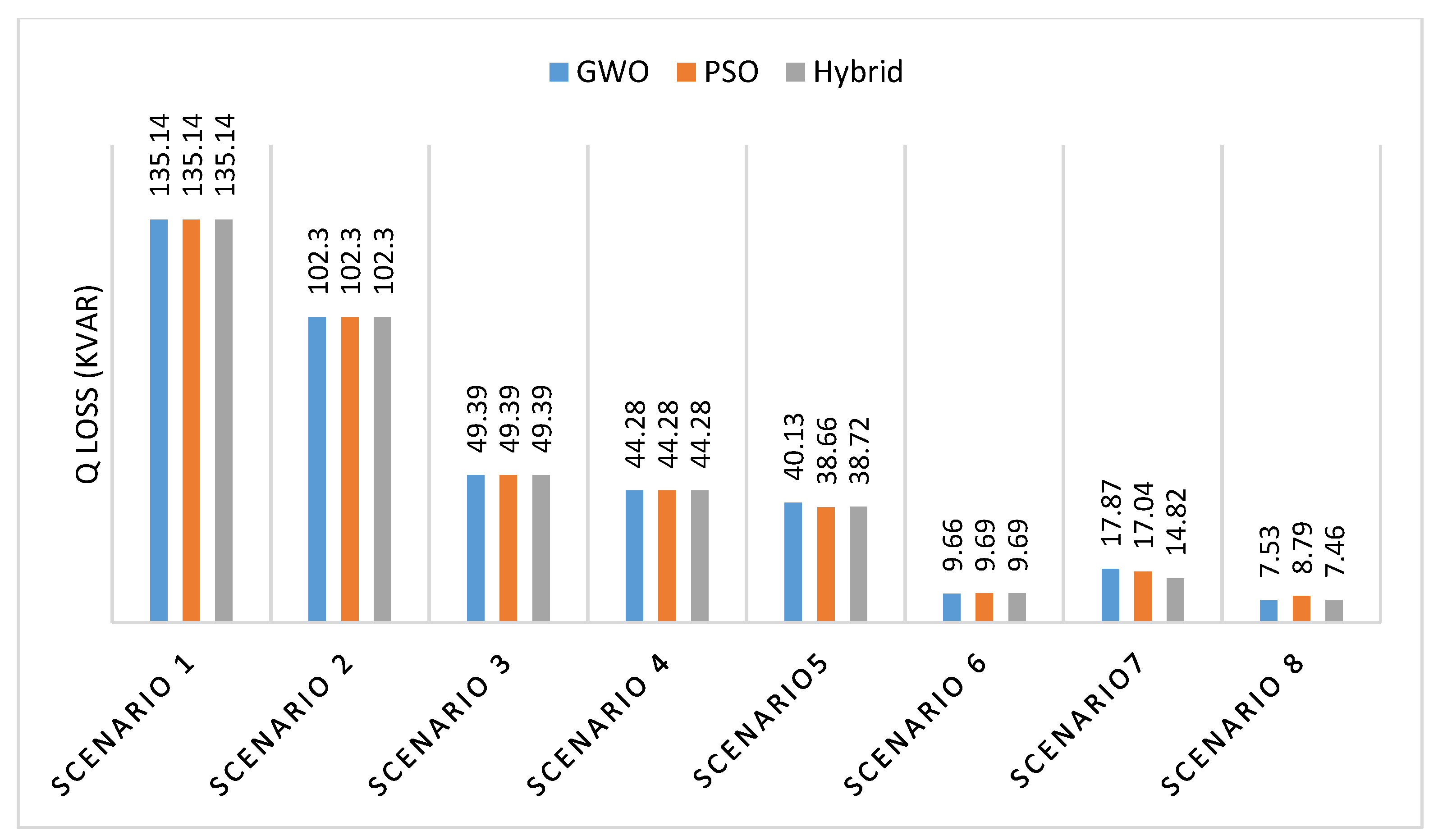From Figure 5, base case reactive loss is 135.141 kVar, which is reduced to 102.305, 49.3921, 44.2868, 38.7201, 9.6926, 14.8282, and 7.4668 for scenarios 2, 3, 4, 5, 6, 7, and 8, respectively using the proposed hybrid technique. It is clearly observed that scenario 7 the injection of active and reactive power after system reconfiguration increases the reactive power losses. 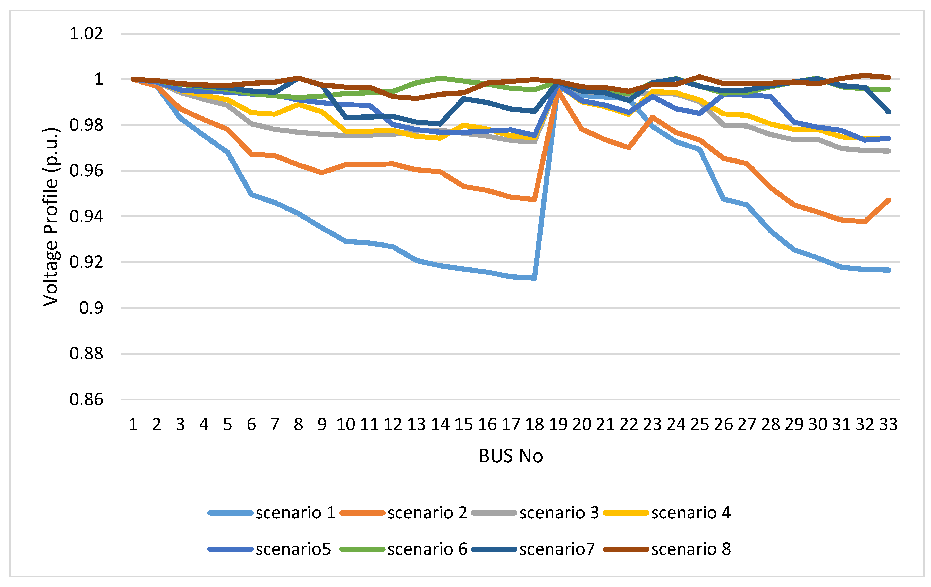Voltage profile curves for all scenarios are shown in Figure 6. It is clearly indicated that the system voltage profile for scenario 8 is the best. The minimum voltage magnitude of the network is 0.91309 (p.u.), which is improved to 0.93782, 0.96867, 0.97406, 0.97344, 0.99206, 0.98051, and 0.99165 using scenarios 2, 3, 4, 5, 6, 7, and 8, respectively. In order to show the performance of the proposed hybrid GWO-PSO, some of the results are compared to different techniques for only for scenarios as the last three scenarios are not illustrated in the compared reference in

Table 4. Comparison of methods performance for the 33-bus system.

Scenarios		Proposed Hybrid GWO-PSO	FWA [30]	HSA [30]	GA [30]	RGA [30]
Scenario 2	Switches opened	7, 9, 14, 32, 37	7, 9, 14, 32, 28	7, 9, 14, 32, 37	33, 34, 9, 36, 28	7, 9, 14, 32, 37
	P loss (kW)	139.55	139.98	138.06	141.60	139.46
	Reduction%	31.14%	30.93%	31.88%	30.15%	31.20%
	${\mathrm{V}}_{\mathrm{worst}}$ (p.u.)	0.93782	0.9413	0.9342	0.9310	0.9315
Scenario 3	Switches opened	33, 34, 35, 36, 37	33, 34, 35, 36, 37	33, 34, 35, 36, 37	33, 34, 35, 36, 37	33, 34, 35, 36, 37
	P loss (kW)	71.4571	88.68	96.76	100.1	97.60
	Reduction%	64.74%	56.24%	52.26%	50.60%	51.84%
	${\mathrm{V}}_{\mathrm{worst}}$ (p.u.)	0.96867	0.9680	0.9670	0.9605	0.9687
Scenario 4	Switches opened	7, 9, 14, 32, 37	7, 9, 14, 32, 28	7, 9, 14, 32, 37	33, 34, 9, 36, 28	7, 9, 14, 32, 37
	P loss (kW)	58.8769	83.91	97.13	98.36	98.23
	Reduction%	70.95%	58.59%	52.07%	51.46%	51.53%
	${\mathrm{V}}_{\mathrm{worst}}$ (p.u.)	0.97406	0.9612	0.9479	0.9506	0.9479
Scenario 5	Switches opened	11, 28, 30, 33, 34	7, 14, 11, 32, 28	7, 14, 10, 32, 28	7, 34, 10, 32, 28	7, 12, 9, 32, 27
	P loss (kW)	50.8905	67.11	73.05	75.13	74.32
	Reduction%	74.89%	66.89%	63.95%	62.92%	63.33%
	${\mathrm{V}}_{\mathrm{worst}}$ (p.u.)	0.97344	0.9713	0.9700	0.9766	0.9691

. Table 4 shows that the proposed hybrid technique has a greater power loss percentage reduction than FWA for scenario 2, 3, 4, and 5. Comparing the results of percentage reduction in power loss between the proposed hybrid GWO-PSO and FWA, it is observed that the GWO-PSO results are 31.14%, 64.74%, 70.95%, and 74.89%, however, the FWA are [30] is 30.93%, 56.24%, 58.59%, and 66.89% for scenarios 2, 3, 4, and 5. It is observed that the performance of the proposed technique is better than FWA, HSA, GA, and Refined Genetic Algorithm (RGA) in terms of power loss minimization. The authors [30] use sensitivity analysis to identify DG allocation and use one of the optimization methods to find size of the DG. Figure 7 shows the conversion characteristics of GWO, PSO, and hybrid GWO-PSO for scenario 8. PSO reaches a reasonable solution but not the optimal. GWO and hybrid technique reach the optimal solution. It can be observed that the proposed hybrid technique provides the best improvement for both the optimal solution and convergence speed.

5.2. IEEE 69-Bus Test System

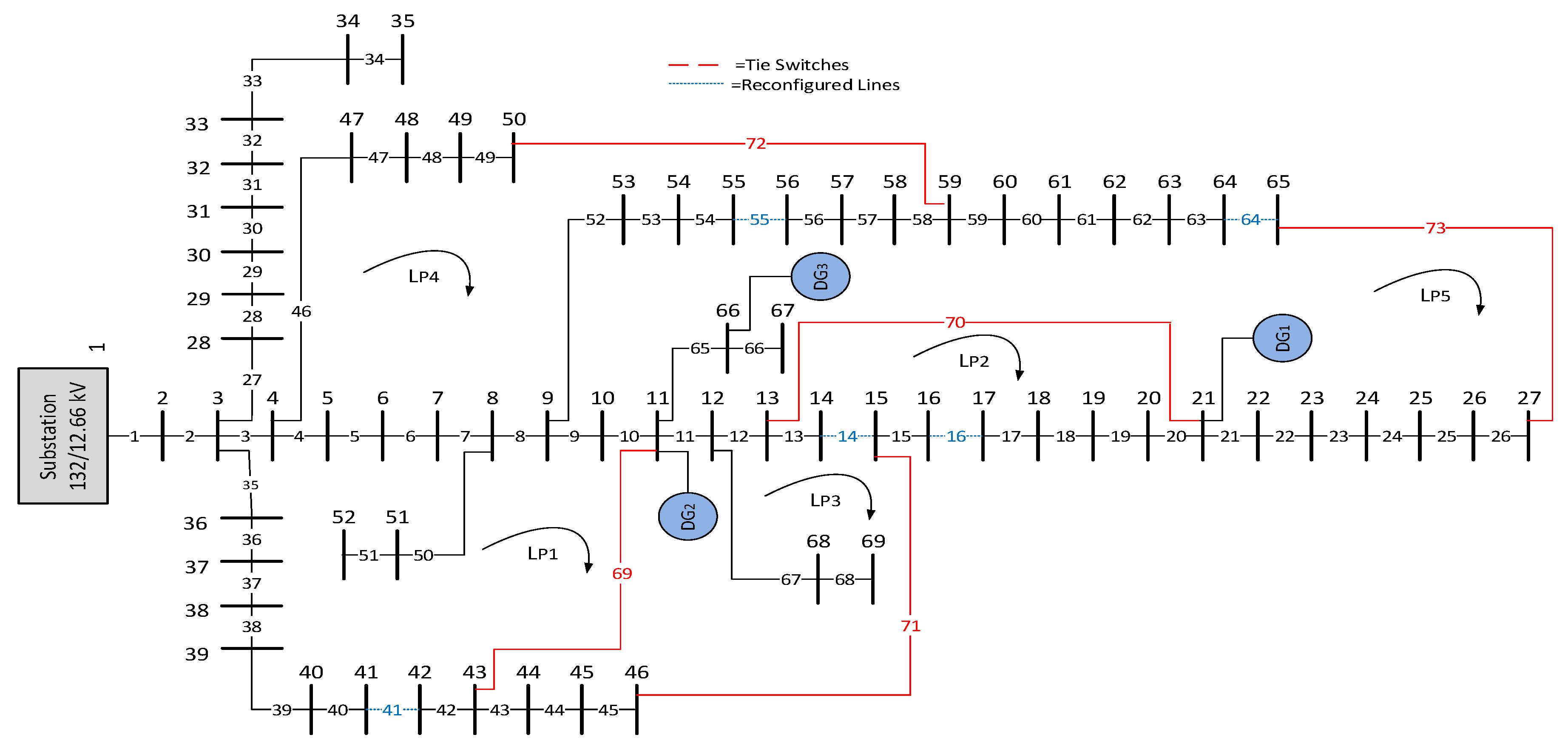
The system base configuration is having 1–68 sectionalize switches normally closed and 69–73 tie switches are normally opened. The total real and reactive power loads are 3.8 MW and 2.69 MVAR, respectively. The system base capacity is 100 MVA and base voltage is 12.66 KV. The limits of real and reactive power injected by DGs are same as test system A. Figure 8 shows the single line diagram for scenario 8. In order to compare the performance of hybrid GWO-PSO, all scenarios are simulated with GWO and PSO results are provided in

Table 5. Comparison of simulation results for P-type DG units of the 69-bus system.

Scenarios		GWO	PSO	Proposed Hybrid GWO-PSO
Scenario 1	Switches opened	69, 70, 71, 72, 73	69, 70, 71, 72, 73	69, 70, 71, 72, 73
	P loss (KW)	224.9295	224.9295	224.9295
Scenario 2	Switches opened	14, 57, 61, 69, 70	14, 57, 61, 69, 70	14, 57, 61, 69, 70
	P loss (KW)	98.5687	98.5687	98.5687
	reduction%	56.17%	56.17%	56.17%
	Iterations	300	200	30
Scenario 3	Switches opened	69, 70, 71, 72, 73	69, 70, 71, 72, 73	69, 70, 71, 72, 73
	DG size in MW (bus)	0.5223 (18), 1.7779 (61), 0.0257 (68)	0.3992 (18), 1.7269 (61), 0.4596(66)	0.5271 (11), 1.7189 (61), 0.3799(18)
	P loss (KW)	71.4131	69.6525	69.3873
	reduction%	68.25%	69.03%	69.15%
	Iterations	300	300	100
Scenario 4	Switches opened	14, 57, 61, 69, 70	14, 57, 61, 69, 70	14, 57, 61, 69, 70
	DG size in Mw (bus)	1.4344 (61), 0.5670 (27), 1.0457(2)	1.4339 (61), 0.5659 (27), 0.6146 (51)	1.4341 (61), 0.5661 (27), 0.5374 (11)
	P loss (KW)	39.0186	36.7430	35.5060
	reduction%	82.65%	83.66%	84.21%
	Iterations	200	200	50
Scenario 5	Switches opened	14, 57, 61, 69, 70	13, 56, 61, 69, 70	14, 55, 61, 69, 70
	DG size in MW (bus)	1.4339 (61), 0.5659 (27), 0.5375 (11)	1.4339 (61), 0.5694 (27), 0.6072 (51)	1.4340 (61), 0.4902 (64), 0.5375 (11)
	P loss (KW)	35.5060	36.7412	35.1337
	reduction%	84.21%	83.66%	84.38%
	Iterations	8000	8000	2000

and

Table 6. Comparison of simulation results for PQ⁺-type DG units of the 69-bus system.

Scenarios		GWO	PSO	Proposed Hybrid GWO-PSO
Scenario 6	Switches opened	69, 70, 71, 72, 73	69, 70, 71, 72, 73	69, 70, 71, 72, 73
	DG size in MVA (bus)	0.0006 + j 0.0711 (69) 1.6913 + j 1.2438 (61) 0.7718 + j 0.2386 (68)	0.4402 + j 0.3143 (36) 1.7345 + j 1.2383 (61) 0.5219 + j 0.3530 (17)	0.4530 + j 0.3219 (68) 1.6917 + j 1.2081 (61) 0.3180 + j 0.2111 (21)
	P loss (KW)	9.5920	7.1709	4.4863
	reduction%	95.73%	96.81%	98.00%
	Iterations	300	300	100
Scenario 7	Switches opened	14, 57, 61, 69, 70	14, 57, 61, 69, 70	14, 57, 61, 69, 70
	DG size in MVA (bus)	0.0871 + j 0.2096 (68) 1.4155 + j 1.0131 (61) 0.5643 + j 0.3856 (27)	0.6137 + j 0.4385 (51) 1.4171 + j 1.01236 (6) 0.5629 + j 0.3904 (27)	0.5366 + j 0.3826 (11) 1.4167 + j 1.0129 (61) 0.5629 + j 0.3900 (27)
	P loss (KW)	8.4784	7.7388	5.8868
	reduction%	96.23%	96.55%	97.38%
	Iterations	300	300	100
Scenario 8	Switches opened	8, 13, 20, 24, 55	12, 21, 40, 53, 70	14, 16, 41, 55, 64
	DG size in MVA (bus)	0.08778 + j 0.5722 (2) 0.8475 + j 0.5899 (11) 1.7651 + j 1.2605 (61)	1.7298 + j 1.2346 (61) 0.7649 + j 0.5493 (50) 0.7791 + j 0.5339 (43)	0.4319 + j 0.2913 (21) 0.5897 + j 0.4161 (11) 1.6770 + j 1.1979 (61)
	P loss (KW)	5.4798	4.40472	3.7132
	reduction%	97.56%	98.04%	98.34%
	Iterations	10000	10000	3000

. The population size using all the techniques is 50, 50, 50, 100, 60, 60, and 100 in scenarios 2 to 8, respectively. The proposed hybrid technique shows the least iteration numbers for all of the scenarios, similar to the IEEE 33-bus system. From Table 5 and Table 6, base case power loss is 224.9295 kW, which is reduced to 3.7132 using scenarios 8 with percentage reduction 98.34% by integration of DG with PQ+ and system reconfiguration simultaneously. From Figure 9, Scenario 7 shows that power loss for PQ+ type DG installation after reconfiguration is not less than the DG installation before reconfiguration and the best improvement in power loss reduction is for scenario 8. 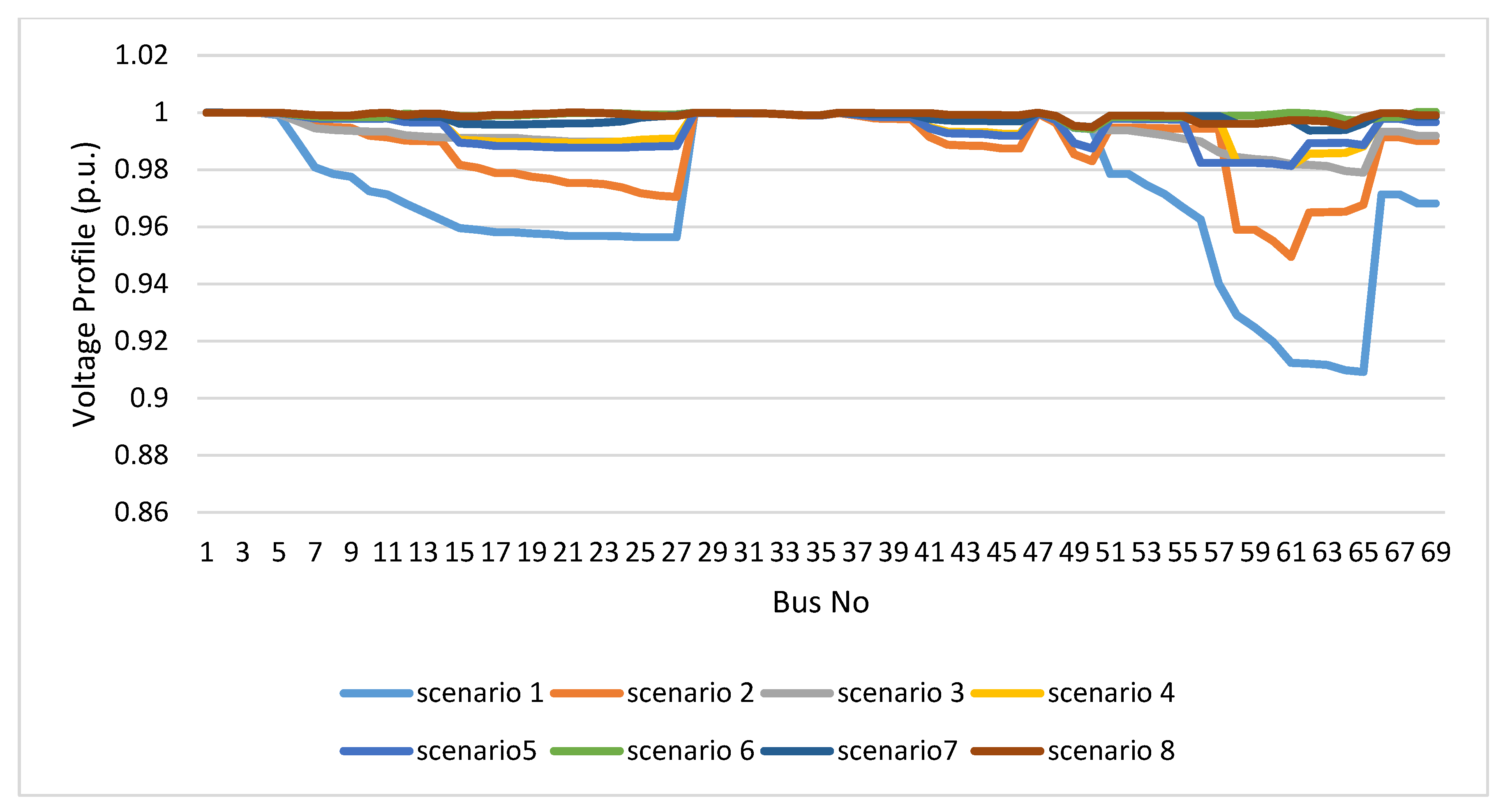From Figure 10, base case reactive loss is 102.1456 kVar, which is reduced to 92.0237, 34.9527, 34.1729, 34.2659, 7.2140, 6.8968, and 5.6053 using scenarios 2 to 8, respectively. Voltage profile curves for all scenarios are shown in Figure 11. It is indicated that system voltage profile for scenario 8 is the best same as the 33-bus test system. The minimum voltage magnitude of the network is 0.90919 (p.u.), which is improved to 0.94947, 0.97898, 0.98134, 0.98133, 0.99426, 0.99369, and 0.99486 for scenarios 2 to 8, respectively, using the proposed hybrid technique. Some of the results are compared to results from previous analysis using different techniques for only four scenarios as in

Table 7. Comparison of methods performance for the 69-bus system.

Scenarios		Proposed Hybrid GWO-PSO	FWA [30]	HSA [30]	GA [30]	RGA [30]
Scenario 2	Switches opened	14, 57, 61, 69, 70	14, 56, 61, 69, 70	69, 18, 13, 56, 61	69, 70, 14, 53, 61	69, 17, 13, 55, 61
	P loss (kW)	98.5687	98.59	99.35	103.29	100.28
	Reduction%	56.17%	56.17%	55.85%	54.08%	55.42%
	${\mathrm{V}}_{\mathrm{worst}}$ (p.u.)	0.94947	0.9495	0.9428	0.9411	0.9428
Scenario 3	Switches opened	69, 70, 71, 72, 73	69, 70, 71, 72, 73	69, 70, 71, 72, 73	69, 70, 71, 72, 73	69, 70, 71, 72, 73
	P loss (kW)	69.3873	77.85	86.77	88.5	87.65
	Reduction%	69.15%	65.39%	61.43%	60.66%	61.04%
	${\mathrm{V}}_{\mathrm{worst}}$ (p.u.)	0.97898	0.9740	0.9677	0.9687	0.9678
Scenario 4	Switches opened	14, 57, 61, 69, 70	14, 56, 61, 69, 70	69, 18, 13, 56, 61	69, 70, 14, 53, 61	69, 17, 13, 55, 61
	P loss (kW)	35.5060	43.88	51.30	54.53	52.34
	Reduction%	84.21%	80.49%	77.20%	75.76%	76.73%
	${\mathrm{V}}_{\mathrm{worst}}$ (p.u.)	0.98134	0.9720	0.9619	0.9401	0.9611
Scenario 5	Switches opened	14, 55, 61, 69, 70	69, 70, 13, 55, 63	69, 17, 13, 58, 61	10, 15, 45, 55, 62	10, 16, 14, 55, 62
	P loss (kW)	35.1337	39.25	40.30	46.20	44.23
	Reduction%	84.38%	82.55%	82.08%	73.38%	80.32%
	${\mathrm{V}}_{\mathrm{worst}}$ (p.u.)	0.98133	0.9796	0.9736	0.9727	0.9742

. Table 7 shows that the percentage power loss reduction for proposed hybrid technique at 69-bus is lower than the FWA technique. Figure 12 shows the conversion characteristics of GWO, PSO, and hybrid GWO-PSO for scenario 8. It can be observed from Figure 12 that the GWO and PSO reach a reasonable solution but not the optimal. Moreover, PSO is faster than GWO. Also, the proposed hybrid technique provides the best improvement for both optimal solution and convergence speed.

5.3. The 78-Bus Real Test System

This system test data is a real recorded data from the distribution system of Cairo and it is given in

Table A1. Test data for a 78-bus system.

Switch No.	From bus i	To bus i + 1	Ri, i + 1	Xi, i + 1	P(KW)	Q(kVar)
1	1	2	0.178125	0.241746	685.8921	298.3631
2	2	3	0.016875	0.022902	685.8921	298.3631
3	3	4	0.0525	0.071251	717.069	311.925
4	4	5	0.0125	0.016965	748.2459	325.487
5	5	6	0.0125	0.016965	174.5907	75.94696
6	6	7	0.00875	0.011875	286.8276	124.77
7	7	8	0.02	0.027143	748.2459	325.487
8	8	9	0.03	0.040715	244.427	106.3257
9	9	10	0.06125	0.083127	255.6507	111.2081
10	10	11	0.04375	0.059376	1153.546	501.7924
11	11	12	0.015625	0.021206	236.9446	103.0709
12	12	13	0.055625	0.075492	265.0038	115.2766
13	13	14	0.0175	0.02375	717.069	311.925
14	14	15	0.02	0.027143	685.8921	298.3631
15	3	16	0.008125	0.011027	717.069	311.925
16	16	17	0.0375	0.050894	685.8921	298.3631
17	17	18	0.025	0.033929	436.4768	189.8674
18	1	19	0.13125	0.178128	286.8276	124.77
19	19	20	0.0125	0.016965	729.5398	317.3498
20	20	21	0.03375	0.045804	717.069	311.925
21	21	22	0.00375	0.005089	271.2392	117.989
22	22	23	0.06625	0.089912	654.7152	284.8011
23	23	24	0.06875	0.093305	685.8921	298.3631
24	24	25	0.0525	0.071251	717.069	311.925
25	25	26	0.0125	0.016965	748.2459	325.487
26	26	27	0.0975	0.132324	729.5398	317.3498
27	27	28	0.05375	0.072948	735.7752	320.0622
28	28	29	0.00625	0.008482	654.7152	284.8011
29	29	30	0.10625	0.144199	249.4153	108.4957
30	30	31	0.025	0.033929	467.6537	203.4294
31	31	52	0.01875	0.025447	1153.546	501.7924
32	32	15	0.02	0.027143	149.6492	65.0974
33	32	16	0.055	0.074644	202.6499	88.15273
34	24	32	0.015	0.020358	277.4745	120.7014
35	1	33	0.1375	0.186611	685.8921	298.3631
36	33	34	0.03125	0.042412	779.4229	339.0489
37	34	35	0.04	0.054287	286.8276	124.77
38	35	36	0.06375	0.086519	685.8921	298.3631
39	36	37	0.0025	0.003393	748.2459	325.487
40	37	38	0.0375	0.050894	717.069	311.925
41	38	39	0.00875	0.011875	717.069	311.925
42	39	40	0.0875	0.118752	723.3044	314.6374
43	40	41	0.02125	0.02884	654.7152	284.8011
44	41	42	0.005	0.006786	748.2459	325.487
45	42	43	0.05375	0.072948	717.069	311.925
46	43	25	0.0375	0.050894	748.2459	325.487
47	1	44	0.019625	0.026634	748.2459	325.487
48	44	45	0.0225	0.030536	685.8921	298.3631
49	45	46	0.1225	0.166253	748.2459	325.487
50	46	47	0.015	0.020358	685.8921	298.3631
51	47	48	0.09125	0.123842	174.5907	75.94696
52	48	49	0.01375	0.018661	717.069	311.925
53	49	50	0.0625	0.084823	717.069	311.925
54	50	51	0.0375	0.050894	174.5907	75.94696
55	51	52	0.025	0.033929	717.069	311.925
56	1	53	0.03625	0.049197	221.3561	96.2899
57	53	54	0.04375	0.059376	729.5398	317.3498
58	1	55	0.05	0.067858	717.069	311.925
59	55	56	0.025	0.033929	236.9446	103.0709
60	56	57	0.01625	0.022054	26.81215	11.66328
61	57	58	0.08125	0.11027	748.2459	325.487
62	58	59	0.00625	0.008482	685.8921	298.3631
63	59	60	0.01125	0.015268	1122.369	488.2305
64	60	61	0.04875	0.066162	1122.369	488.2305
65	61	62	0.005	0.006786	374.123	162.7435
66	62	63	0.015	0.020358	685.8921	298.3631
67	63	64	0.09375	0.127235	1122.369	488.2305
68	64	65	0.06875	0.093305	685.8921	298.3631
69	65	66	0.025	0.033929	1091.192	474.6685
70	66	67	0.015625	0.021206	748.2459	325.487
71	67	68	0.053125	0.0721	143.4138	62.38501
72	68	69	0.0375	0.050894	1122.369	488.2305
73	69	70	0.039375	0.053438	685.8921	298.3631
74	61	54	0.05375	0.072948	1091.192	474.6685
75	1	71	0.15625	0.212058	717.069	311.925
76	71	72	0.12625	0.171342	685.8921	298.3631
77	72	73	0.015	0.020358	1028.838	447.5446
78	73	74	0.06875	0.093305
79	74	75	0.01875	0.025447
80	75	76	0.0625	0.084823
81	76	77	0.1525	0.206968
82	77	78	0.02	0.027143

. The system base configuration consists of having 1–78 sectionalized switches normally closed, whereas five switches are normally opened. The total real and reactive power loads are 48.25 MW and 20.99 MVAR, respectively. The system base capacity is 1.5 MVA and base voltage is 22 KV. The limits of real and reactive power injected by DGs are 0 to 20 MW and 0 to 10 MVAR, respectively.

Table 8. Comparison of simulation results for P-type DG units of the 78-bus system.

Scenarios		GWO	PSO	Proposed Hybrid GWO-PSO
Scenario 1	Switches opened	32, 34, 40, 48, 63	32, 34, 40, 48, 63	32, 34, 40, 48, 63
	P loss (KW)	421.7192	421.7192	421.7192
Scenario 2	Switches opened	10, 28, 34, 45, 64	10, 28, 34, 45, 64	10, 28, 34, 45, 64
	P loss (KW)	209.3731	209.3731	209.3731
	reduction%	50.3525%	50.3525%	50.3525%
	Iterations	100	100	30
Scenario 3	Switches opened	32, 34, 40, 48, 63	32, 34, 40, 48,63	32, 34, 40, 48, 63
	DG size in MW (bus)	6.6347 (67), 9.4411 (5), 13.0352 (29)	6.6392 (67), 8.3307 (32), 11.4460 (52)	9.0871 (7), 13.0333 (29), 6.6383 (67)
	P loss (KW)	142.0250	154.9977	141.9624
	reduction%	66.32%	63.24%	66.33%
	Iterations	300	300	100
Scenario 4	Switches opened	10, 28, 34, 45, 64	10, 28, 34, 45, 64	10, 28, 34, 45, 64
	DG size in Mw (bus)	5.4594 (75), 10.5558 (3), 6.5508 (67)	5.1046 (43), 10.3781 (16), 6.55061 (67)	5.5491 (25), 10.3774 (16), 6.5501 (67)
	P loss (KW)	107.6866	109.2588	107.6448
	reduction%	74.4648%	74.092%	74.47%
	Iterations	300	300	100
Scenario 5	Switches opened	8, 23, 30, 43, 64	8, 26, 34, 41, 64	8, 23, 30, 43, 64
	DG size in MW (bus)	15.8913 (32), 5.4580 (75), 6.5507 (67)	9.1835 (32), 5.8525 (31), 6.9573 (25)	6.5505 (67), 5.4581 (75), 15.8910 (32)
	P loss (KW)	88.9550	115.6147	88.9550
	reduction%	78.90%	72.5849%	78.90%
	Iterations	8000	8000	3000

and

Table 9. Comparison of simulation results for PQ⁺-type DG units of the 78-bus system.

Scenarios		GWO	PSO	Proposed Hybrid GWO-PSO
Scenario 6	Switches opened	32, 34, 40, 48, 63	32, 34, 40, 48, 63	32, 34, 40, 48, 63
	DG size in MVA (bus)	4.2811 + j 0.0002 (11) 6.2412 + j 4.5606 (3) 12.9952 + j 5.6954 (29)	7.0371 + j 3.0773 (31) 9.0865 + j 3.9673 (7) 8.3189 + j 3.6267 (25)	13.0438 + j 5.7339 (29) 6.6376 + j 2.8963 (67) 9.0840 + j 3.9653 (7)
	P loss (KW)	123.0646	101.6025	89.2335
	reduction%	70.81%	75.91%	78.84%
	Iterations	300	300	100
Scenario 7	Switches opened	10, 28, 34, 45, 64	10, 28, 34, 45, 64	10, 28, 34, 45, 64
	DG size in MVA (bus)	6.5494 + j 2.7644 (67) 5.4412 + j 0.0273 (75) 10.5141 + j 4.5881 (3)	10.3709 + j 4.5219 (16) 5.1071 + j 2.2269 (43) 6.5514 + j 2.8547 (67)	6.5530 + j 2.8517 (67) 10.3680 + j 4.5201 (16) 5.5462 + j 2.4208 (25)
	P loss (KW)	92.9695	90.3978	88.4952
	reduction%	77.95%	78.56%	79.01%
	Iterations	300	300	100
Scenario 8	Switches opened	8, 21, 42, 55, 63	8, 20, 41, 51, 63	8, 20, 42, 55, 63
	DG size in MVA (bus)	5.4565 + j 2.3783 (75) 18.2086 + j 7.9589 (32) 6.6405 + j 2.8940 (67)	6.6404 + j 2.8937 (67) 16.2463 + j 7.0932 (24) 5.7228 + j 2.4958 (31)	18.4208 + j 8.0511 (24) 6.6400 + j 2.8937 (67) 5.4565 + j 2.3779 (75)
	P loss (KW)	48.93	61.5560	48.6045
	reduction%	88.39%	85.40%	88.47%
	Iterations	9000	9000	3000

illustrate the comparison in the same way as test systems A and B. As shown in Table 8 and Table 9, base case power loss is 421.7192 kW, which is reduced to 48.6045 using scenario 8, i.e., a percentage power loss reduction of 88.47%. The base case reactive loss is 572.3431 KVar which is reduced to 65.9645 Kvar. System losses are very small compared to the load capacity due to the fact that the loads are industrial and are located directly after the substation. Figure 13 shows that power loss reduction for scenario 8 is higher than any other scenario as it performs the system reconfiguration, sizing, and siting of DGs in parallel. Figure 14 shows the reactive power loss from different scenarios using the three optimization techniques. Comparing the results from the hybrid technique it can been clearly seen that the reactive power loss is reduced to 284.1545, 192.6667, 146.0921, 120.7269, 121.1049, 120.1029, and 65.9645 for scenarios 2 to 8, respectively, using the proposed hybrid technique. Voltage profile curves for all scenarios are shown in Figure 15. Similar to test systems A and B, the voltage profile for scenario 8 is the best. The minimum voltage magnitude of the network is 0.97046 (p.u.), which is improved to 0.99139, 0.98552, 0.99161, 0.99231, 0.99161, 0.99161, and 0.99598 using scenarios 2, 3, 4, 5, 6, 7, and 8, respectively. The population size using all techniques is 50, 60, 60, 100, 60, 60, and 100 in scenarios 2 to 8, respectively. Tables show that the proposed hybrid technique takes the least number of iterations for the most of the scenarios, similar to the two IEEE test systems. 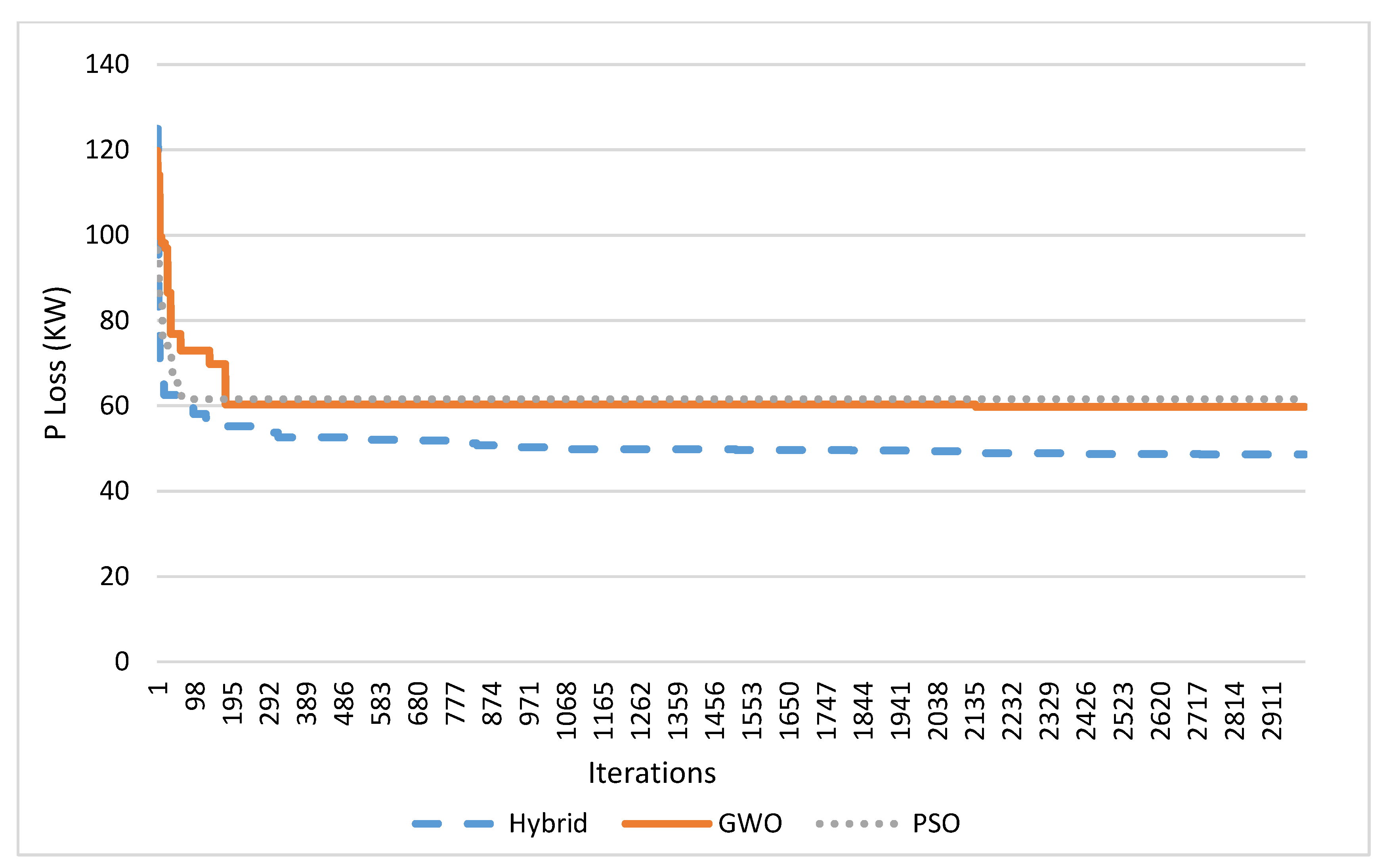Figure 16 shows the conversion characteristics of GWO, PSO, and hybrid GWO-PSO for scenario 8 where GWO and PSO did not reach the optimal solution. PSO is faster than GWO. However, GWO is with a better solution than PSO. Furthermore, the proposed technique shows the best results compared to the results obtained from the IEEE test systems.

This work presents system reconfiguration and DGs allocation and sizing for 33-bus and 69-bus IEEE systems and a 78-real distribution system located in Cairo, Egypt. The presented study proposes a new hybrid GWO-PSO technique. The validity of the technique is held by comparing the performance of the proposed new hybrid GWO-PSO technique to GWO and PSO individually for the same objective function of minimization of power losses. This combination of the two metaheuristic techniques leads to the elimination of the disadvantages of both techniques, the minimization of the number of iterations and helps reach the optimal solution at every simulation. This paper also compares the proposed technique to the results obtained from previous work in terms of power loss minimization.

In the IEEE 33-bus system, active power loss decreases from 202.67 to 8.1962 kW, reactive power loss decreases from 135.141 to 7.4668 kVar and the minimum voltage magnitude improved from 0.91309 to 0.99165 (p.u.) relative to the scheme without considering system reconfiguration and DG placement.

In the IEEE 69-bus system, active power loss decreases from 224.9295 to 3.7132 kW, reactive power loss decreases from 102.1456 to 5.6053 kVar, and the minimum voltage magnitude improved from 0.90919 to 0.99486 (p.u.).

In the 78-bus real system, active power loss decreases from 421.7192 to 48.6045 kW, reactive power loss decreases from 572.3431 to 65.9645 kVar and the minimum voltage magnitude increased from 0.97046 to 0.99598 (p.u.).

From the later results, it is observed that using power loss as an objective function improves all the other elements of the network. Moreover, the combination of network reconfiguration and optimal placement of DG units has the best improvement compared to solving each one of them separately. The results show that the performance of the proposed hybrid GWO-PSO technique is better than the other techniques in terms of number of iteration, conversion speed, and power loss minimization.

6. Conclusions

This paper presents a new hybrid GWO-PSO technique used to optimally allocate and size DGs in order to reduce power losses. It considers large search spaces system reconfiguration and DG allocation and sizing for 33-bus and 69-bus IEEE systems and a 78-bus real distribution system located at Cairo, Egypt. The validity of the technique is held by comparing the performance of the proposed new hybrid GWO-PSO technique to GWO and PSO individually. This combination of the two metaheuristic techniques leads to the elimination of the disadvantages of each technique when applied individually, reduces the number of iterations, and ensures that the optimal solution is reached during every simulation.

To check the validity of the proposed technique, results were compared to a reference that uses sensitivity analysis to identify DG allocation and optimization methods to find size of the DG. This comparison showed that the performance of the proposed technique outperformed FWA, HSA, GA, and Refined Genetic Algorithm (RGA) in terms of power loss minimization.

Hybrid PSO-GWO; although PSO is a very fast optimization technique, it may sometimes do not reach the optimal solution in large search spaces. Consequently, this does not allow GWO to reach the optimal solution. Thus, it is observed that initializing the hybridization by GWO leads to better results than by PSO as GWO is more accurate than PSO in large searching spaces.

Furthermore, the case studies also showed that the proposed technique is faster and requires a smaller number of iterations that applying PSO or GWO individually. On one hand, although PSO reaches a reasonable solution faster than the GWO technique, it is not reliable as it may not reach the optimum in all cases. On the other hand, the GWO technique reaches a more accurate solution than PSO in all cases despite the system size. Therefore, due to the nature of the nonlinear behavior of the problem and the size of the systems used, running GWO or PSO optimization particularly will not lead to the same results at each run and may not reach the optimal solution. Thus, the results may be averaged to increase the accuracy.