A Novel Control Strategy for Grid-Connected Inverter Based on Iterative Calculation of Structural Parameters

Abstract

A novel control strategy that is based on iterative calculation of structural parameters is proposed for grid-connected inverter in this paper. The proposed strategy has a good dynamic performance, which makes it particularly suitable for the application of PV grid-connected generation. First, a second-order discretization mathematical model of grid-connected inverter control is established in the dq frame. The corresponding relation between the control signal and the output current is deduced in formulas. Then, the values of structural parameters in the formulas can be obtained through iterative calculation, which can further reduce the amount of calculation. After several iteration cycles, the structural parameters are approximately equal to their actual values and the inverter can be controlled as an open-loop system with its dynamic performance optimized. At last, simulation and experiments are performed. The results show that the static performance of the proposed strategy is as good as that of the classical ones, but its dynamic performance is improved significantly.

1. Introduction

With the rapid developing of distributed photovoltaic generation, grid-connected inverters are widely used [1,2], and the control strategies of grid-connected inverters are very important in the renewable energy development. There are three basic control strategies for grid-connected inverter: (1) classical grid-current control strategy, (2) droop or damping control strategy [3], and (3) some other intelligent control strategies.

In classical grid-current control strategy, PI(D) or PR controllers are used in the dq or αβ frame. Ref. [4] pointed out that a PI(D) controller can realize the no-error tracking of constant signal, so it is used in the dq frame, in which the three-phase sine signals are transformed into two constant signals. While [5] revealed that a PR controller can realize the no-error tracking of sin signal, so it is used in the αβ frame. Recently, most of the related research focuses on improving its dynamics performance. In [6], the PR controller was optimized to be an adaptive one by using a conventional SRF phase-locked loop (PLL), so the dynamics performance of the grid-connected inverter was improved when the target output currents changed. However, since it was based on PLL, if the grid frequency changed, the output of the inverter might be affected. Ref. [7] presented a systematic procedure for accurate dynamics assessment and a tuning of synchronous-frame PI current controllers, based on linear control for multiple-input–multiple-output (MIMO) systems. The research realized to reduce sampling frequency while maintaining dynamic performance. If the sampling frequency remained, then the dynamic performance would be improved. However, it was designed for wind power, it remains to be proved whether it is fit for PV generation. Ref. [8] presented a two-step controller design approach, its detailed modeling, and in-depth dynamic analysis. The controller was designed based on the fourth-order system when considering the dynamics of the output LCL filter. The strategy can improve the dynamic performance, but it is a high order control system, which makes it difficult to be realized. In summary, the classical grid-current control strategy is the most common strategy, which can achieve steady state control without error. However, there will be inescapable overshoot and oscillation in the output if the target is always changing. In the application of photovoltaic generation, because of the randomness of light intensity, the target output currents of a grid-connected inverter often change dramatically. So, the disadvantages of poor dynamic performance of PI controller are magnified in photovoltaic generation. The dynamic performance of PV grid-connected inverter is still to be optimized.

In droop or damping control strategy, the inverters are always working as voltage sources. Ref. [9] proposed a voltage-type droop control method for parallel inverters. It can help the inverters to share power without interconnection. But, in this method, the line impedance participates in computation, which is difficult to measure in practice. Among all of the droop or damping control strategy, the virtual synchronous generator (VSG) draws the most research interests. In [10], some characteristics of mechanical generators, such as the rotational inertia and damping coefficient, are added to the frequency and voltage regulation control of grid-connected inverter, to compensate for the lack of inertia in power electronics. Therefore, the distributed inverters get the function of frequency and voltage regulation. However, the DC power supply is batteries, not PV cells. Ref. [11] proposed a self-adaptive inertia and damping combination control of VSG with an interleaving control technique. It makes a contribution to supporting frequency stability. Nevertheless, the article did not mention what kind of DC power supply was used. Ref. [12] proposed a new control strategy based on the analysis of excitation state for VSG. It can improve its low-voltage ride-through (LVRT) capability. However, it still requires the DC power supply is controllable. Ref. [13] used VSG in a microgrid based on PV/BES system and revealed directly that SVG requires the controllability of active power output from DC power supply, because it is involved in active power–frequency regulation. In summary, the droop or damping control strategy, such as SVG, is suitable for distributed energy storage system or photovoltaic system with energy storage, but not for pure photovoltaic system.

Some intelligent control methods have been applied to grid-connected control in recent years, such as fuzzy control [14], sliding mode control [15], model predictive control (MPC), and so on. Ref. [16] is a survey on various intelligent control methods. It provides plenty of detailed information, especially on MPC. Ref. [17,18] used MPC to control grid-connected high-power four-level diode-clamped inverters. Ref. [17] focused on active and reactive power control and [18] applied it on wind energy conversion systems. They detailed the MPC process: The controller uses all the possible switching states (at least six different states) of the inverter for the prediction and evaluates them using a cost function. The switching state, which minimizes the cost function, is then chosen and applied at the next sampling interval. Nevertheless, they also pointed out that without modulation, at least six switching states should be evaluated in every sampling interval, thus the controller needs to do more calculation than usual. Ref. [19] evaluated the dynamic performance of an MPC-based 9-phase flux-switching permanent-magnet motor drive, concluded that after using MPC the dynamic performance of the 9P-FSPM was improved drastically, however, since it is a 9-phase system, there were so many switching states that the controller was difficult to bear the computation burden. Ref. [20,21] both compared MPC and PI-PWM in different applications to prove that the dynamic performance is much better than that of PI. Without the modulation process, it needs to do six predictive calculations and compare all the results before every control signal is output. Ref. [22] proposed an optimized MPC method based on approximate dynamic programming. It was proved to reduce the computation burden, but the computation is still larger than other control methods with modulation processes. In summary, MPC is a competitive alternative control method with satisfying dynamic performance, but without modulation, it makes the computation burden heavier.

In this paper, a novel control strategy for grid-connected inverter based on iterative calculation of structural parameters is proposed. The core idea of this strategy is to obtain the accurate real-time values of the structural parameters in the exact mathematical model of a grid-connected inverter, so that the inverter can be controlled as an open-loop system to improve its dynamic performance. Because some structural parameters cannot be measured directly, the controller needs to do iterative calculation to approach the actual values of the structural parameters. In the process of iterative calculation, the structural parameters are varying very slightly, so the controller can use the values of input and output in the last iterative cycle to calculate the values of structural parameters in this cycle. Use the values of structural parameters in this cycle to calculate the appropriate control signal for the next iteration cycle.

In Section 2, a model of grid-connected inverter in dq-frame is established, the corresponding relation between control signal and output current is deduced in formulas. Then, the undetermined structural parameters are pointed out and their calculation formulas are given. Next, the process of the iterative calculation control strategy is described in detail, and the initialization is described additionally. In Section 3 and Section 4, both simulation and experimental results are presented, confirming the pretty good dynamic performance. Finally, the conclusions are summarized in Section 5.

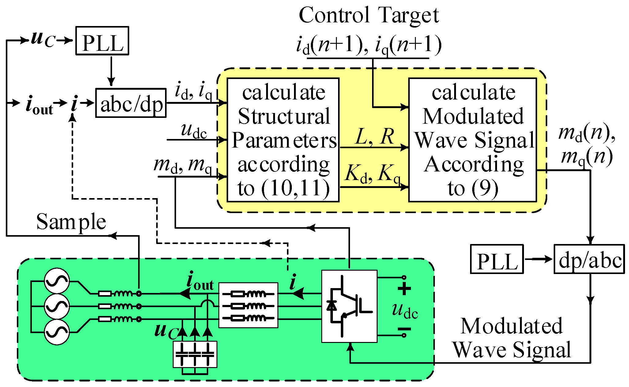
2. The Proposed Novel Control Strategy

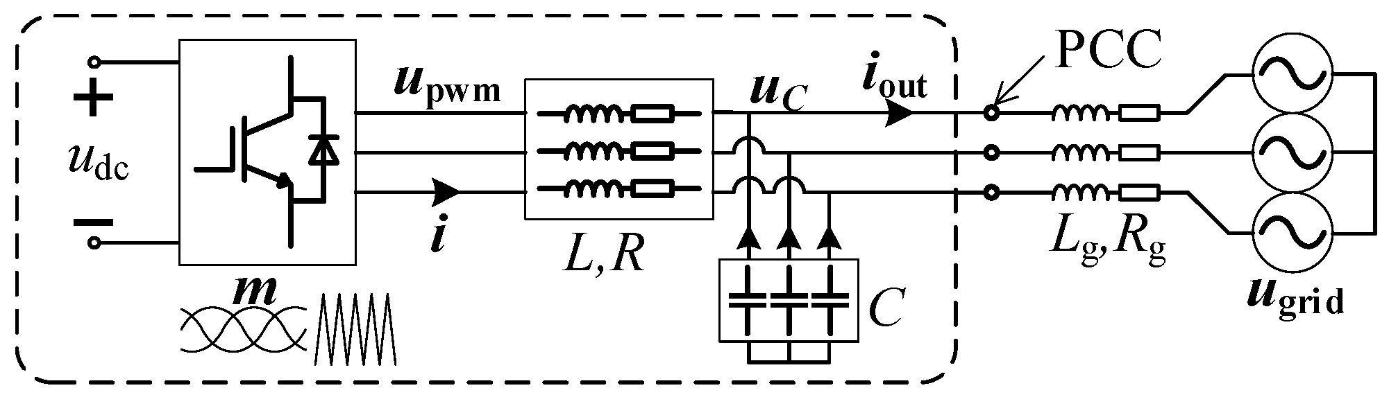
2.1. The Dq-Frame Model of Grid-Connected Inverter

The grid-connected inverter model is shown in Figure 1, where m is the given modulated wave, u_pwm is the fundamental component of the voltage waveform directly generated at the outlet of the inverter bridge, and i is the fundamental component of the current waveform in the filter inductor. It is considered that u_grid is an ideal sine wave voltage source, the inverter is connected to the grid at PCC, u_C is the voltage of PCC, and i_out is the actual grid-connected current.

The AC voltage and current respectively, satisfy the vector formulas (1):

$$\{\begin{array}{l}{\overrightarrow{i}}_{\mathrm{out}}=\overrightarrow{i}+C·\frac{\mathrm{d}{\overrightarrow{u}}_C}{\mathrm{d}t}\\ {\overrightarrow{u}}_{\mathrm{pwm}}=R·\overrightarrow{i}+L·\frac{\mathrm{d}\overrightarrow{i}}{\mathrm{d}t}+{\overrightarrow{u}}_C\end{array}$$

(1)

In the rotating dq frame, (1) can be translated into (2) and (3), where i_d, i_q are, respectively, the components of i on dq axis.

$$\{\begin{array}{l}{i}_{\mathrm{out}\_\mathrm{d}}=i_{\mathrm{d}}-\omega C·u_{C\mathrm{q}}-C·\frac{\mathrm{d}{u}_{C\mathrm{d}}}{\mathrm{d}t}\\ i_{\mathrm{out}\_\mathrm{q}}=i_{\mathrm{q}}+\omega C·u_{C\mathrm{d}}-C·\frac{\mathrm{d}{u}_{C\mathrm{q}}}{\mathrm{d}t}\end{array}$$

(2)

$$\{\begin{array}{l}{u}_{\mathrm{pwm}\_\mathrm{d}}=R·i_{\mathrm{d}}-\omega L·i_{\mathrm{q}}+u_{C\mathrm{d}}+L·\frac{\mathrm{d}{i}_{\mathrm{d}}}{\mathrm{d}t}\\ u_{\mathrm{pwm}\_\mathrm{q}}=R·i_{\mathrm{q}}+\omega L·i_{\mathrm{d}}+u_{C\mathrm{q}}+L·\frac{\mathrm{d}{i}_{\mathrm{q}}}{\mathrm{d}t}\end{array}$$

(3)

(2) shows that there is a determined mapping relation between i and i_out. In general, the value of the filter capacitor C in the inverter is relatively accurate and it can be considered as a fixed value, and u_C can be obtained by real-time measurement. Therefore, i_out can be controlled indirectly by directly controlling i, and i can also be obtained indirectly by observing the real-time value of i_out. So, the following sections of this article are mainly focusing on the control of i.

As for (3), in an inverter control system, u_pwm cannot be artificially set directly, but it can be determined by the product of m, u_dc and other factors, as shown in (4), where u_{pwm_d}, u_{pwm_q}, and m_d, m_q are, respectively, the components of u_pwm and m on the dq axis.

$$\{\begin{array}{l}{u}_{\mathrm{pwm}\_\mathrm{d}}=K_{\mathrm{d}}·u_{\mathrm{dc}}·m_{\mathrm{d}}\\ u_{\mathrm{pwm}\_\mathrm{q}}=K_{\mathrm{q}}·u_{\mathrm{dc}}·m_{\mathrm{q}}\end{array}$$

(4)

In (4), K_d and K_q are defined as the gain coefficients of the inverter bridge and K_d, K_q are related to the range of the carrier wave variation, but they do not have an absolute positive correlation. If the range of carrier wave variation is fixed, K_d, K_q take a small range near a certain value. Define this value as the central value K of the gain coefficient of the inverter bridge. K is related to the upper and lower limits of the carrier wave. In (5), max and min are defined to represent the upper and lower limits of the carrier wave.

$$K_{\mathrm{d}},K_{\mathrm{q}}\approx \frac{1}{\max -\min }=K$$

(5)

For example, if the carrier wave is a triangular wave ranging from −1 to +1, K_d, K_q ≈ 1/2 = K.

When considering the voltage of PCC, u_C is taken as the 0-phase reference, the q-axis component u_Cq of u_C in (3) is always equal to 0. Combining (3) and (4), the dq-frame model of grid-connected inverter can be formulated in (6):

$$\{\begin{array}{l}{K}_{\mathrm{d}}·u_{\mathrm{dc}}·m_{\mathrm{d}}=R·i_{\mathrm{d}}-\omega L·i_{\mathrm{q}}+L·\frac{\mathrm{d}{i}_{\mathrm{d}}}{\mathrm{d}t}+u_{C\mathrm{d}}\\ K_{\mathrm{q}}·u_{\mathrm{dc}}·m_{\mathrm{q}}=R·i_{\mathrm{q}}+\omega L·i_{\mathrm{d}}+L·\frac{\mathrm{d}{i}_{\mathrm{q}}}{\mathrm{d}t}\end{array}$$

(6)

Discretize (6), we get (7). Then, transfer (7), we get (8) finally.

$$\{\begin{array}{l}{K}_{\mathrm{d}}{u}_{\mathrm{dc}}{m}_{\mathrm{d}}(n)=R{i}_{\mathrm{d}}(n)-\omega L{i}_{\mathrm{q}}(n)+\frac{L}{T_s}[i_{\mathrm{d}}(n+1)-i_{\mathrm{d}}(n)]+u_{C\mathrm{d}}\\ K_{\mathrm{q}}{u}_{\mathrm{dc}}{m}_{\mathrm{q}}(n)=R{i}_{\mathrm{q}}(n)+\omega L{i}_{\mathrm{d}}(n)+\frac{L}{T_s}[i_{\mathrm{q}}(n+1)-i_{\mathrm{q}}(n)]\end{array}$$

(7)

$$\{\begin{array}{l}{i}_{\mathrm{d}}(n+1)=i_{\mathrm{d}}(n)+\frac{T_s}{L(n)}[K_{\mathrm{d}}(n)u_{\mathrm{dc}}(n)m_{\mathrm{d}}(n)-R(n)i_{\mathrm{d}}(n)+\omega L(n)i_{\mathrm{q}}(n)-u_{C\mathrm{d}}(n)]\\ i_{\mathrm{q}}(n+1)=i_{\mathrm{q}}(n)+\frac{T_s}{L(n)}[K_{\mathrm{q}}(n)u_{\mathrm{dc}}(n)m_{\mathrm{q}}(n)-R(n)i_{\mathrm{q}}(n)-\omega L(n)i_{\mathrm{d}}(n)]\end{array}$$

(8)

In (8), i_d(n + 1), i_q(n + 1) are the control targets and m_d(n), m_q(n) are the only two parameters that can be set artificially or software-automatically. There is also a determined mapping relation between i_d(n + 1), i_q(n + 1) and m_d(n), m_q(n). If we want the inverter to output a certain target current defined through i_d(n + 1) and i_q(n + 1), we just need to set m_d(n) and m_q(n) according to (9), where i_d(n + 1) − i_d(n) and i_q(n + 1) − i_q(n) are abbreviated as $\Delta$i_d(n) and $\Delta$i_q(n), respectively.

$$\{\begin{array}{l}{m}_{\mathrm{d}}(n)=\frac{L}{T_s{K}_{\mathrm{d}}{u}_{\mathrm{dc}}}\Delta i_{\mathrm{d}}(n)+\frac{R}{K_{\mathrm{d}}{u}_{\mathrm{dc}}}{i}_{\mathrm{d}}(n)-\frac{\omega L}{K_{\mathrm{d}}{u}_{\mathrm{dc}}}{i}_{\mathrm{q}}(n)+\frac{1}{K_{\mathrm{d}}{u}_{\mathrm{dc}}}{u}_{C\mathrm{d}}\\ m_{\mathrm{q}}(n)=\frac{L}{T_s{K}_{\mathrm{q}}{u}_{\mathrm{dc}}}\Delta i_{\mathrm{q}}(n)+\frac{R}{K_{\mathrm{q}}{u}_{\mathrm{dc}}}{i}_{\mathrm{q}}(n)+\frac{\omega L}{K_{\mathrm{q}}{u}_{\mathrm{dc}}}{i}_{\mathrm{d}}(n)\end{array}$$

(9)

2.2. The Structural Parameters to Be Determined

It is represented in (8) that m_d(n) and m_q(n) can be proposed by the control system according to the corresponding target i_d(n + 1), i_q(n + 1), only if all the parameters in (8) are known. Most of the parameters can be obtained by real-time measurement, such as i_d(n), i_q(n), u_dc, u_Cd, and $\omega$. However, others cannot be measured in real time, such as R, L, and K_d, K_q. All these four parameters are used to describe the characteristics of inverter structure itself, so we define them as Structural Parameters.

L and R are both physical quantities, but the actual value of L is affected by the current passing through itself depending on the hysteresis loop, similarly the actual value of R is affected by the temperature. So, both of them will vary slightly when the current is changing, and cannot be measured directly when the inverter is running. K_d and K_q change randomly and slightly near the central value K. So, the four structural parameters are always varying slightly and slowly. Although they are important to the control system, they remain to be determined. If we obtain the certain values of the structural parameters, then the inverter can be controlled as expected. Thus, how to determine the structural parameters is the key in the proposed control strategy.

Discretize the structural parameters in (8) or (9), we get R(n), L(n) in (10), and K_d(n), K_q(n) in (11).

$$\{\begin{array}{c}L(n)=\frac{u_{\mathrm{dc}}{m}_{\mathrm{q}}(n)K_{\mathrm{q}}(n)i_{\mathrm{d}}(n)-u_{\mathrm{dc}}{m}_{\mathrm{d}}(n)K_{\mathrm{d}}(n)i_{\mathrm{q}}(n)+u_{C\mathrm{d}}{i}_{\mathrm{q}}(n)}{\omega \left[i_{\mathrm{d}}{(n)}^2+i_{\mathrm{q}}{(n)}^2\right]+\left[i_{\mathrm{d}}(n)\Delta i{(n)}_{\mathrm{q}}-i_{\mathrm{q}}(n)\Delta i_{\mathrm{d}}(n)\right]/T_s}\\ R(n)=\frac{u_{\mathrm{dc}}{m}_{\mathrm{d}}(n)K_{\mathrm{d}}(n)i_{\mathrm{d}}(n)+u_{\mathrm{dc}}{m}_{\mathrm{q}}(n)K_{\mathrm{q}}(n)i_{\mathrm{q}}(n)-u_{C\mathrm{d}}{i}_{\mathrm{d}}(n)}{i_{\mathrm{d}}{(n)}^2+i_{\mathrm{q}}{(n)}^2+\left[i_{\mathrm{d}}(n)\Delta i_{\mathrm{q}}(n)-i_{\mathrm{q}}(n)\Delta i_{\mathrm{d}}(n)\right]/\omega T_s}\\ +\frac{K_{\mathrm{d}}{u}_{\mathrm{dc}}{u}_{\mathrm{d}}\Delta i_{\mathrm{q}}+K_{\mathrm{q}}{u}_{\mathrm{dc}}{u}_{\mathrm{q}}\Delta i_{\mathrm{d}}-u_{C\mathrm{d}}\Delta i_{\mathrm{q}}}{\omega T_s\left[i_{\mathrm{d}}{(n)}^2+i_{\mathrm{q}}{(n)}^2\right]+i_{\mathrm{d}}(n)\Delta i_{\mathrm{q}}(n)-i_{\mathrm{q}}(n)\Delta i_{\mathrm{d}}(n)}\end{array}$$

(10)

$$\{\begin{array}{l}{K}_{\mathrm{d}}(n)=\frac{R(n)i_{\mathrm{d}}(n)-\omega L(n)i_{\mathrm{q}}(n)+u_{C\mathrm{d}}+L(n)\Delta i_{\mathrm{d}}(n)/T_s}{u_{\mathrm{dc}}{m}_{\mathrm{d}}(n)}\\ K_{\mathrm{q}}(n)=\frac{R(n)i_{\mathrm{q}}(n)+\omega L(n)i_{\mathrm{d}}(n)+L(n)\Delta i_{\mathrm{q}}(n)/T_s}{u_{\mathrm{dc}}{m}_{\mathrm{q}}(n)}\end{array}$$

(11)

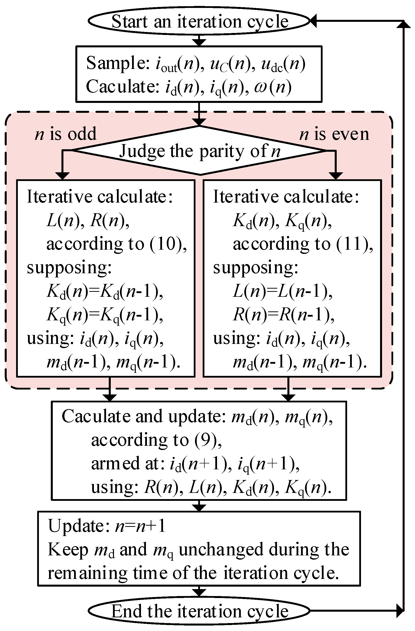
2.3. The Process of Iterative Calculation of Structural Parameters

In general, the dynamic performance of an open-loop system is likely better than that of a closed-loop system, so the main idea of this strategy is to obtain the actual values of the structural parameters, so that the closed-loop system can be treated as an open-loop system to improve its dynamic performance, as shown in the yellow dotted box in Figure 2.

Figure 2 shows the general procedure of the proposed strategy. The inside of the green dotted box is the model of a grid-connected inverter, while outside is the control signal diagram. The voltage and current of PCC are sampled at the beginning of every iteration cycle. Then, we get i_d, i_q, after Park Transformation. Then, use i_d, i_q, m_d, m_q, and u_dc to calculate the structural parameters, L, R, K_d, and K_q, according to (10) or (11). At this moment, the values of m_d, m_q are not updated. They maintain the values of the previous iteration cycle, described as m_d(n − 1), m_q(n − 1). Then, use all the structural parameters to calculate and update m_d(n), m_q(n), according to (9). At last, use m_d, m_q to generate the modulated wave signal, called inverse Park Transformation, and use the modulated wave signal to control IGBT statements.

Inside the yellow dotted box, there are two boxes, which represent the two major parts of the strategy. The outs of one box is exactly the ins of the other. The whole strategy is a circle. That is the process of iterative calculation.

When we calculate the structural parameters, there are four unknown numbers, L, R, and K_d, K_q, but only two equations in both (10) and (11), so we cannot get the unique solution. Fortunately, all of the structural parameters are varying slightly, so L, R can be treated as fixed values, while calculating K_d, K_q according to (11), on the other hand, K_d, K_q can be treated as fixed values, while calculating L, R according to (10). The detailed process is shown in the pink dotted box in Figure 3.

Figure 3 shows the specific procedures of an iteration cycle. Inside the pink dotted box, we use m_d, m_q, and i_d, i_q as the known quantities to calculate the structural parameters, while outside the pink dotted box, we use the structural parameters as known quantities to solve m_d, m_q in software, and output i_d, i_q through hardware. This is called the process of iterative calculation, with the aim of getting accurate values of the structural parameters and controlling the inverter as an open-loop system.

2.4. The Initialization of the Iterative Calculation

In the process of the iterative calculation, the solutions are always used as known quantities, like an algebraic loop, so some of the structural parameters should be initialized at the beginning.

When the system starts computing for the first time, K_d, K_q are initialized to the central value K, and m_d, m_q are set to half of their maximum allowable value. Keep m_d, m_q unchanged until the current is stable, then perform the first iterative calculation to get L, R.

So far, all of the parameters used for the iterative calculation are well prepared, though the structural parameters are not accurate. Then, the controller will carry out the iterative calculation strategy to approach the actual values of the structural parameters, according to Figure 3.

3. Simulation Analysis

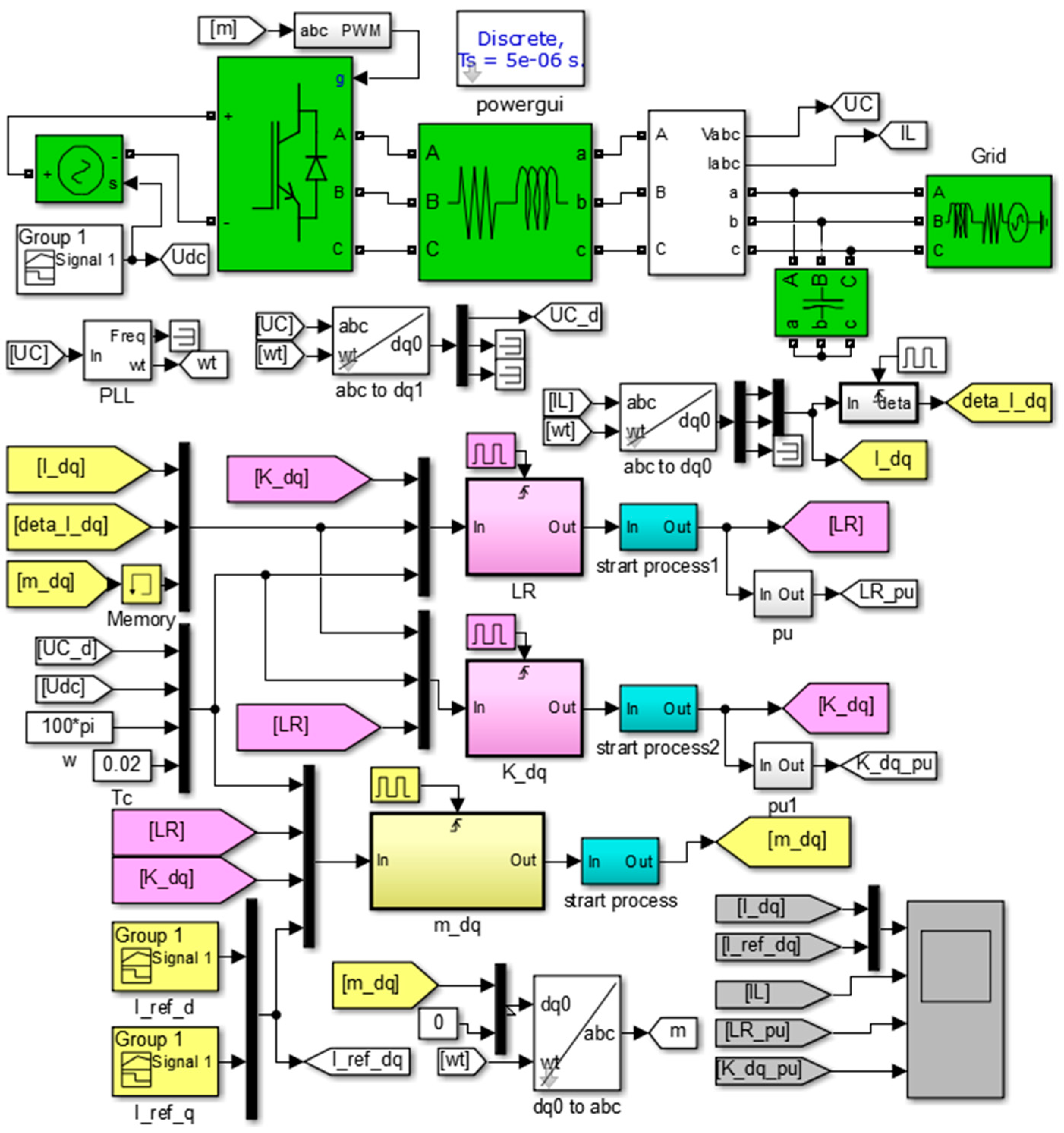
3.1. Simulation Model

In order to verify the effectiveness of the proposed strategy and to analysis the static and dynamic performance of the control effects, a simulation model is established in Matlab/Simulation, according to the model shown in Figure 1. The simulation model is shown in Figure 4. It is the circuit implementation of the formulas and logical relationships that are deduced in Section 2. We can see the ins and outs of every part clearly.

In Figure 4, the green boxes are the power circuit of a grid-connected inverter, the yellow ones show the process of in iterative calculation, the pink ones show the process of calculating structural parameters in batches, and the blue ones show the initialization of the iterative calculation. All modules are in the same colors as the corresponding ones in Figure 2 and Figure 3, except for the start process modules in blue.

All of the main parameters in the simulation model are shown in

Table 1. Simulation parameters.

Parameters		Values
DC Voltage	(udc)	700 ± 50	V
Filter Inductor	(L)	5	mH
Parasitic Resistance	(R)	0.1	$\Omega$
Filter Capacitor	(C)	150	uF
Grid Inductor	(Lg)	0.4	mH
Grid Resistance	(Rg)	0.01	Ω
Grid Voltage	(Ugrid)	220	V
Carrier Frequency	(fc)	3	kHz
Iteration Cycle Time	(Tc)	0.02	s

.

In Table 1, most simulation parameters are based on actual values in the experimental platform. u_dc is the value of series PV cells. L_g and R_g are not actual values but estimated ones. L_g and R_g are the parameters that cannot be set artificially or measured directly. A good control strategy should be fit for all the reasonable L_g and R_g values.

3.2. Control Effect of the Proposed Strategy

The objective of the first simulation is to present the control effect of the proposed control strategy.

The simulation results are shown in Figure 5. The first screen from top to bottom is the reference and measured values of the d-q components of currents, i; the second screen is the three-phase current values in the filter inductor, i; the third screen is the p.u. of the calculated value of L, R, based on their preset values; and, the fourth screen is the p.u. of K_d, K_q, based on their central value K.

The simulation results are analyzed as follows:

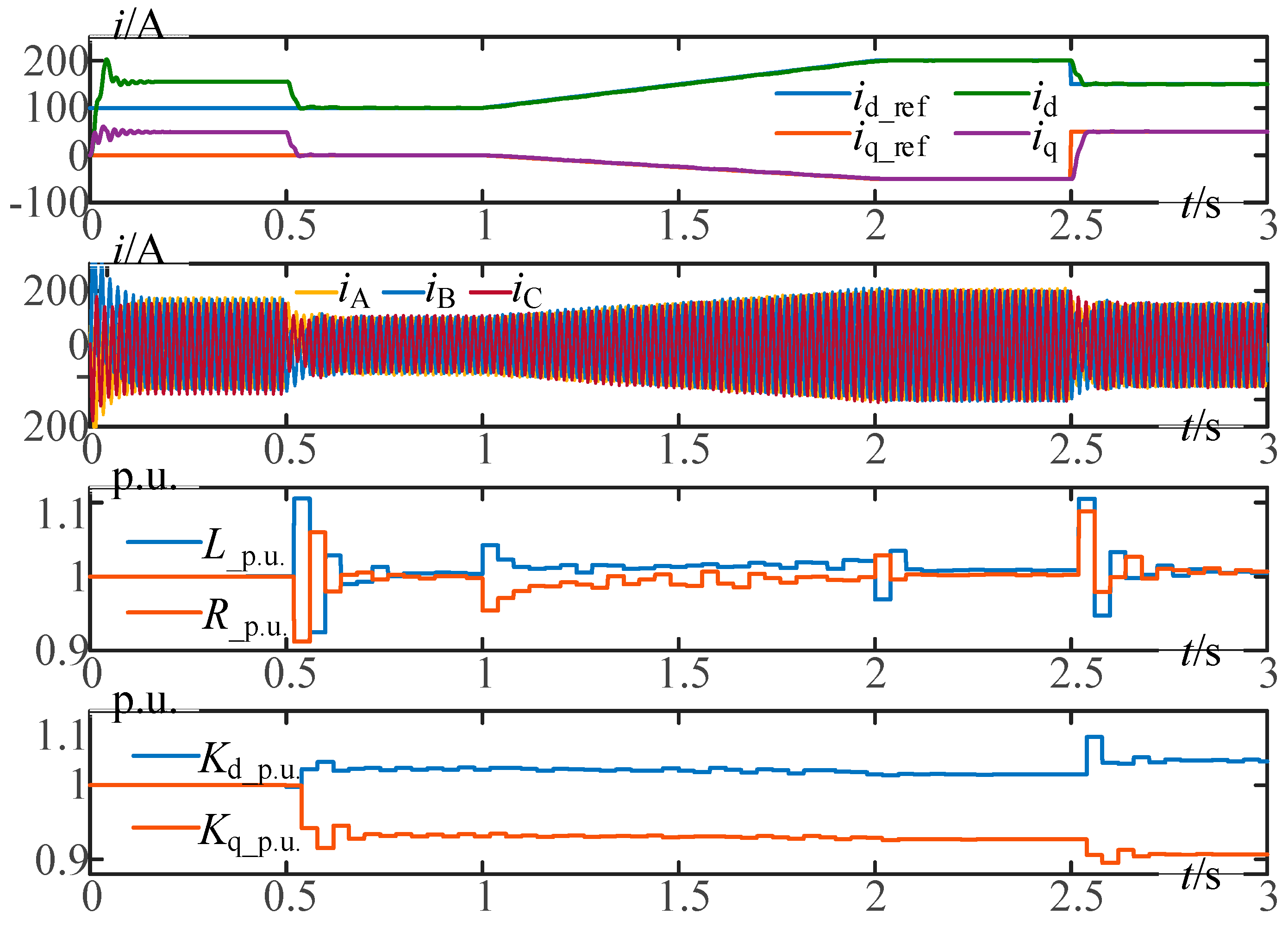
• This simulation shows the control effort of the proposed strategy, including the start-up process, interactive calculate process, and the responses of constants, step functions, and ramp functions.
• The start-up process lasts till 0.5 s. During this period, the inverter output currents do not follow the instruction, because m_d, m_q are set artificially to 0.5. All of the p.u. of structural parameters are calculated according to their preset values, all their standard values are 1. After the current is completely stable around 0.5 s, the iterative calculation starts.
• In the iterative calculation process after 0.5 s, the four structural parameters are all shifting, but the ranges are all small, indicating that the calculated values of the structural parameters are constantly changing, but are not too far from the preset values.
• During 2–2.5 s, the reference current commands are constants. The measured currents are exactly the same as their corresponding reference currents, no-error tracking is achieved. During this period, all of the structural parameters almost do not change after the current is stable. This means the closed-loop system has already been treated as an open-loop one.
• During 1–2 s, the reference current commands are ramp functions. The measured currents are approximately consistent with their corresponding reference currents. This is because the control strategy uses a second-order model, and its $\Delta$i_d(n), $\Delta$i_q(n) remain constant values during a ramp. During this period, the p.u. of structural parameters are varying slightly in a small range, despite the beginning and end points. The p.u. of L, R shift significantly at the beginning and end points, and decay rapidly. This is also because $\Delta$i_d(n), $\Delta$i_q(n) change suddenly at the beginning and end of a ramp, but they will be updated to their suitable values quickly because of the iterative calculation strategy.
• A step occurs in the reference currents at 2.5 s. For the step response, we can see a period of response time, during which the structural parameters undergo large-scale numerical changes. This is because the inverter is treated as an open-loop process. Once the currents suddenly change, the filter inductance will force the currents to generate a DC component at the sudden change point of the phase, and the DC component decays rapidly because of the parasitic resistance, R. The three-phase current imbalance during the response time leads to inaccurate calculations of i_d, i_q, and some other relevant parameters, but they will soon approach anther steady state, as the iterative calculation goes on, as shown in Figure 5.

Therefore, we conclude that:

• The proposed control strategy is effective for grid-connected inverter control.
• The proposed strategy can achieve no-error tracking for constants and ramp functions. The static performance is pretty good.
• During no-error tracking periods, the structural parameters stay fixed or change very little, which means that the closed-loop system has already been treated as an open-loop one.
• During step responses, the structural parameters change largely, and three-phase imbalance occurs in the output currents. The step response of the strategy needs further analysis.

3.3. Details of a Step Response of the Proposed Strategy

The objective of the second simulation is to show the details of a step response of the proposed strategy.

The simulation results are shown in Figure 6, which is the lateral expansion of Figure 5 in only 0.2 s around the step time.

The simulation results are analyzed as follows:

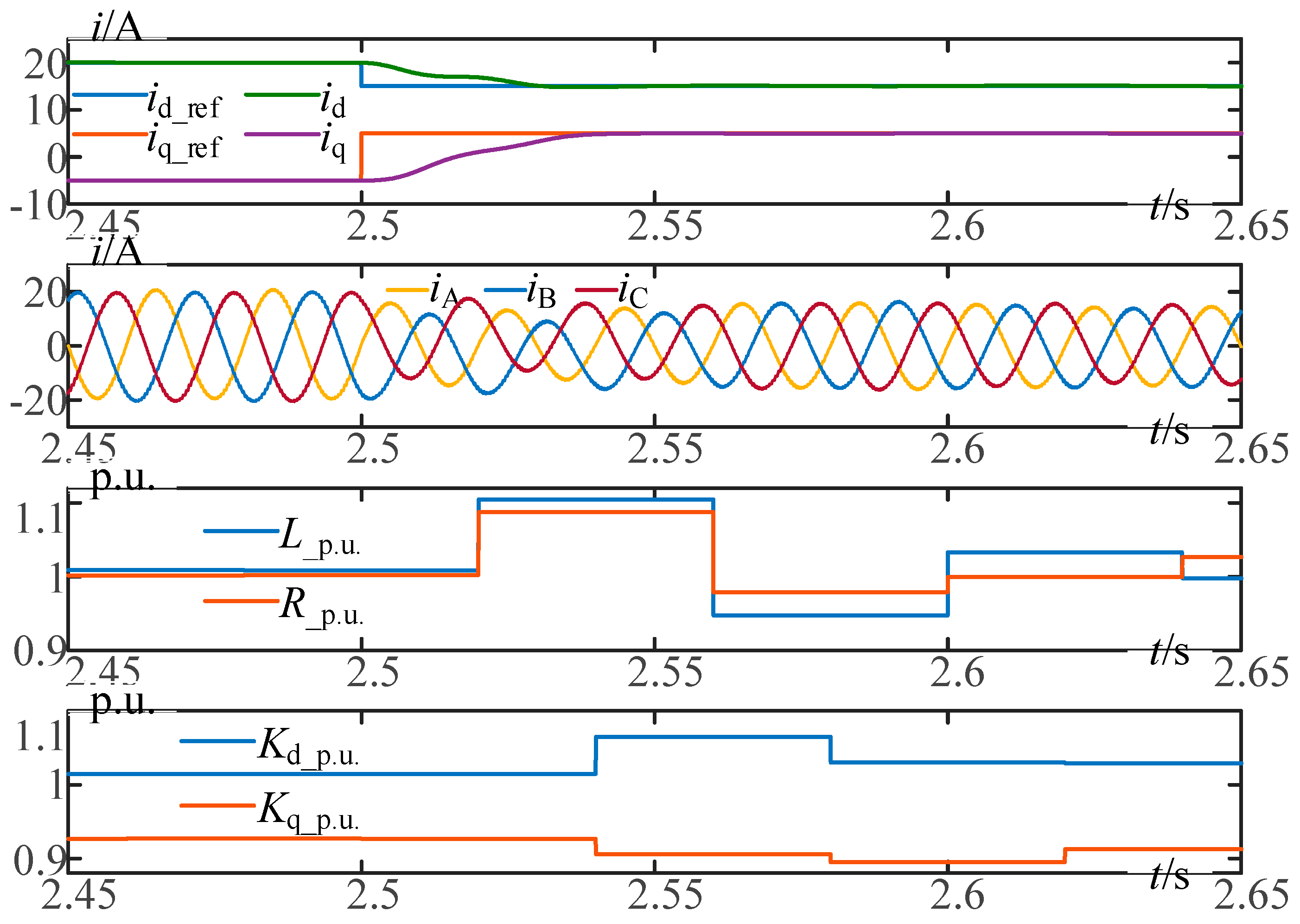
• The step occurs in the 2.5 s target reference current.
• After the step, m_d and m_q immediately update according to (9), using the previous structural parameters. This process can be approximated as an open-loop process. The three-phase currents in the second screen are obviously imbalanced, resulting in the deviations of i_d, i_q in the first screen.
• When comparing the third and the fourth screen, we can see that L, R, and K_d, K_q are updated alternately, which is consistent with the implementation of the strategy, shown in Figure 3.
• When a step occurs, it is necessary to wait until the next iteration cycle to update the values of L, R, and the values of K_d, K_q must wait until the next calculation cycle to be updated. That is the other reason why there is a response time in step response.

And we can conclude that:

• The step response time lasts for about two cycles, during which no overshoot or oscillation, but only three-phase imbalance occurs in the output currents.
• During the step response, the structural parameters are updated in two groups, which means two iteration cycles are needed to complete the response in theory. But in practice, the response time lasts for only one cycle, which will be presented and explained in Section 4: Experimental Results.
• The only drawback of the strategy is three-phase current imbalance during one or two cycles after a step, which has limited negative impacts on grid. Thus, the dynamic performance is satisfying.

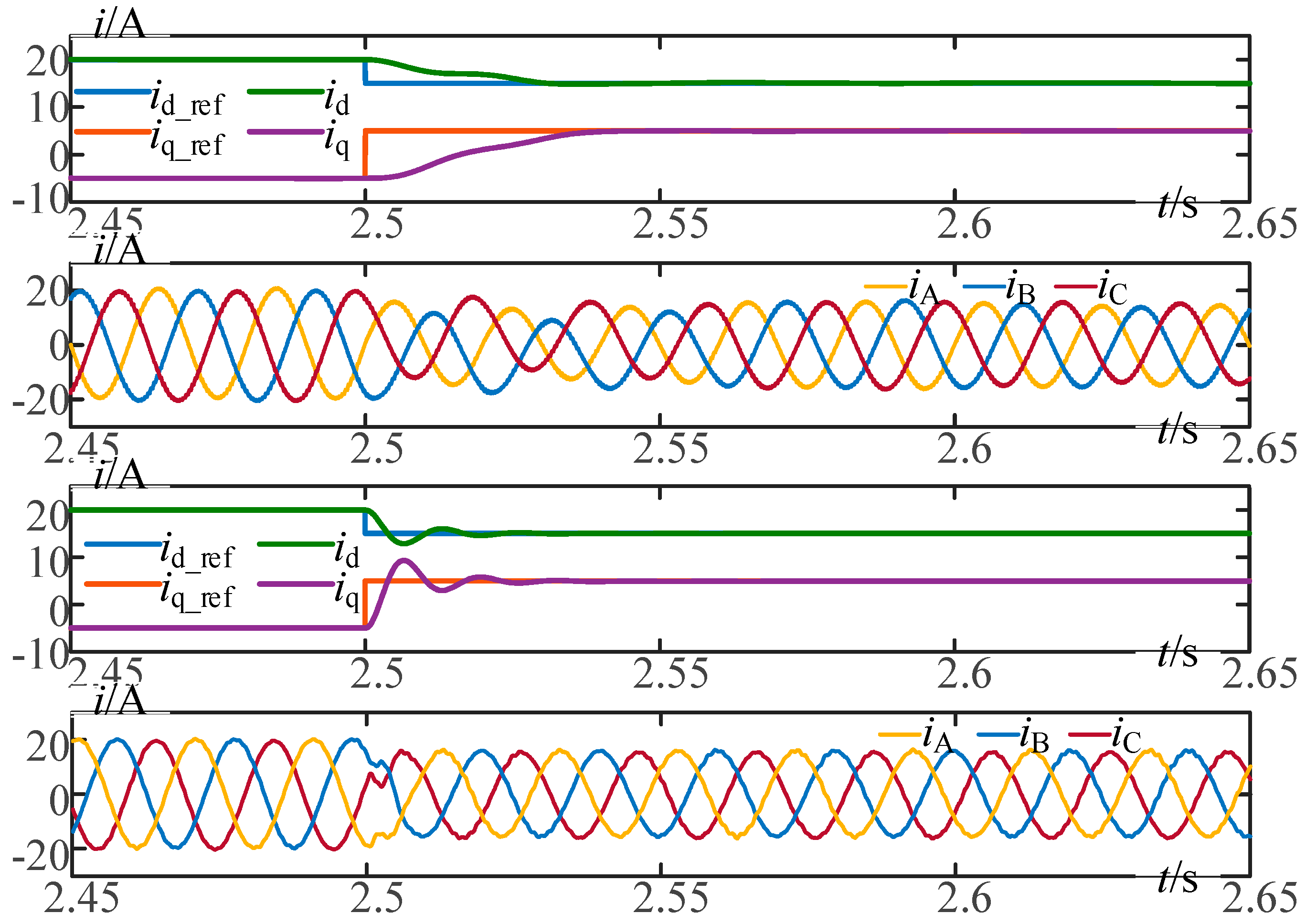
3.4. Comparasion of the Dynamic Performance on a Step Response

The objective of the third simulation is to compare the dynamic performance of the proposed control strategy and a PI controller on the same step response.

The simulation results are shown in Figure 7. The first screen from top to bottom is the reference and measured values of the d-q components of currents, i using the proposed strategy; the second screen is the three-phase current values in the filter inductor, i using the proposed strategy. These two screens are the same as the first two screens in Figure 6. The third screen in Figure 7 is the reference and measured values of the d-q components of currents, i using a PI controller; the fourth screen is the three-phase current values in the filter inductor, i using a PI controller.

The simulation results are analyzed as follows:

• The step response time of PI controller is about two cycles, which is nearly the same as that of the proposed strategy. There are evident overshoot and oscillation during the response time, as seen in the third screen.
• Adjusting PI parameters can affect the dynamic performance of the system to some extent. However, we can never get the ideal step response. Because if we want to improve the response speed, the overshoot and oscillation will intensify. On the other hand, if we want to suppress overshoot and oscillations, the response speed will slow down. Ref. [23] presented the detailed design and implementation of a PI controller for grid-connected inverter. Ref. [24] discussed the design of the digital PI controller used in grid-connected inverter.
• Using the PI controller, the output currents distort severely at the step time, as seen in the fourth screen. If the steps occur frequently for the randomness of sunlight intensity in practice, large amounts of harmonic current will be injected into the grid, which might cause some other serious problems on power quality, such as harmonic resonance.
• Using the proposed strategy, only three-phase current imbalance occurs during the response time, which has minimal negative impact on the grid. The following experimental results will prove and explain that the response time will be shorter in practice than that in simulation.

Then, we can conclude that:

• The disadvantages of a PI controller are overshoot, oscillation and output current distortion, and the distortion might cause worse problem on power quality, such as harmonic resonance.
• The only drawback of the strategy is three-phase current imbalance, which has limited negative impacts on the grid.
• Neither of the methods can provide ideal step responses. Nevertheless, the proposed strategy is better in dynamic performance, for it causes less serious problems to the grid.

4. Experimental Results

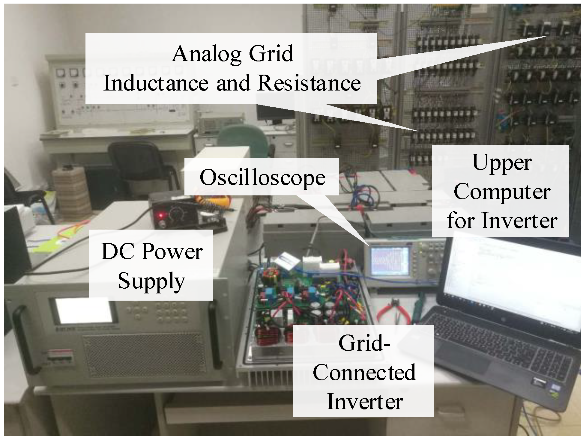
4.1. Experimental Platform

To validate the effectiveness of the proposed strategy, several experiments were conducted on the experimental platform. The experimental platform is shown in Figure 8, consisting of a grid-connected inverter, its upper computer, a DC power supply, an analog power grid, and some other measuring facilities, such as the oscilloscope. The inverter is the core of this experimental platform. All of the other devices are used to service the inverter, and the control strategy is operated in the inverter. All of its control parameters are set according to Table 1. The output voltage of the DC power supply is set to range between 650 V to 750 V. The inductance and resistance of the analog power grid are not set exactly according to Table 1, but tiny values below 1 mH and 0.5 Ω.

4.2. Static Performance

The objective of this experiment is to present the static performance, including no-error tracking and current THD, of the proposed strategy.

In the experiment, the inverter is set to output 5 kW to demonstrate the static performance of the proposed strategy. Its results are shown in Figure 9. (a) and is used to measure the current RMS, and (b) is used for FFT analysis.

The experimental results are analyzed as follows:

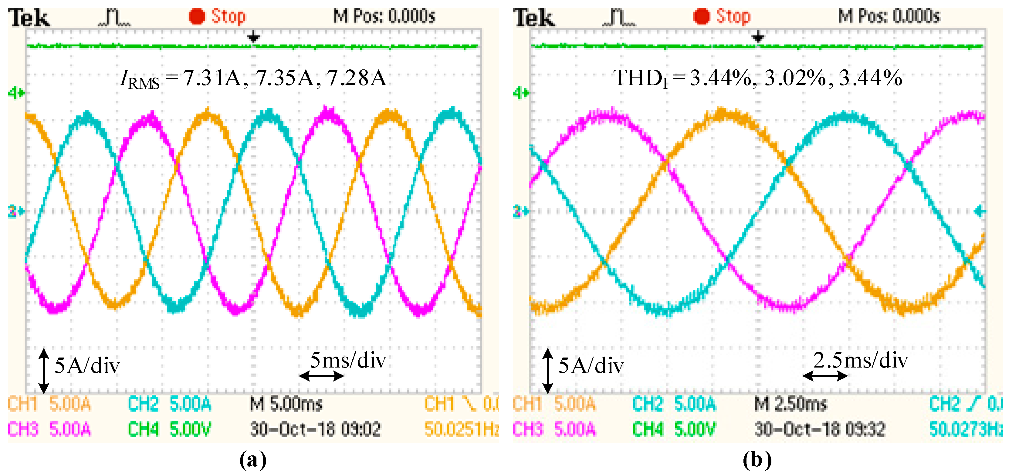
• Figure 9a shows that the measured three-phase current RMS are between 7.28 A to 7.35 A, while the theoretical output current RMS of the 5 kW inverter is 7.597 A, as calculated in (12).

  $$I_{\mathrm{RMS}}=\frac{P_{\mathrm{SUM}}}{\sqrt{3}·U_{\mathrm{Line}}}=\frac{5000\mathrm{W}}{\sqrt{3}\times 380\mathrm{V}}=7.597\mathrm{A}$$

  (12)

  Considering the measurement error and grid voltage deviation (a little higher than rated value, measured about 394 V), the measured values are very close to the theoretical value. This experiment proves that the proposed strategy can achieve static no-error tracking.
• Figure 9b shows the power quality of the output currents. Even though there are some high-order harmonics, the waveforms are already very close to the ideal sine waves, with a THD of less than 3.5%. So, using the proposed strategy, the power quality of the inverter output is pretty good.

We can conclude that:

The strategy can achieve no-error tracking for constants with good power quality of the output currents. So, the static performance of the proposed control strategy is pretty good.

4.3. Dynamic Performance

Since a second-order control model is used in the strategy, it can track a ramp function without error like the response of a constant, which has already been validated both in theory and in simulation. The whole process is too long to appear on the screen of an oscilloscope. Therefore, in this part, only the response of a step function is presented to demonstrate the dynamic performance of the proposed strategy.

The objective of this experiment is to present the dynamic performance on a step response of the proposed strategy.

In the experiment, the inverter is set to output 3.5 kW before the step time and 5 kW after the step time. The experimental results are shown in Figure 10. (a) presents the output currents before and after the step time; Figure 10b is used to analyze three-phase imbalance in output currents.

The experimental results are analyzed as follows:

• In Figure 10a, there is almost no oscillation during the response time. It seems like overshoot, but actually, it is three-phase imbalance, for we can see it clearly in Figure 10d. Both the two auxiliary segments at each time point are of equal length, but one of them cannot touch the boundary waveforms.
• The response time, or three-phase imbalance time, lasts for only one cycle, which is shorter than the simulation results. Theoretically, it needs two-cycle time to complete the iterative calculation and to update of the structural parameters. However, actually, the obvious three-phase imbalance only occurs within one cycle time. The three-phase imbalance may also occur in the following cycle, but it is so inconspicuous that it can be ignored. This is because the actual values of L and R are changing too slightly or slowly to affect the response of a step function, so only the updates of K_d, K_q can affect the response obviously.
• Except for the three-phase current imbalance for only one cycle, there is no other problems on power quality, such as waveform distortion and so on. The three-phase current imbalance has limited effect on the power system, therefore, the proposed control strategy has a good dynamic performance.

Thus, we conclude that:

The dynamic performance of the proposed strategy is satisfying. Because it causes no other power quality problems, but only three-phase current imbalance for only one cycle, which affects the grid very little.

4.4. Comparison with PI Controller

The objective of this experiment is present the control efforts of a PI controller to provide a comparison with the proposed strategy to prove the advantages of the proposed strategy on dynamic performance.

The control effects of the proposed strategy are shown in Figure 10, while the control effects of a typical PI controller are shown in Figure 11 for comparison. All of the experimental parameters and conditions in the two experiments are exactly the same. Figure 11a presents the overshoot and oscillation of the output currents during the step response time; and, Figure 11b presents the sine waveform distortion.

The experimental results are analyzed as follows:

• apparent overshoot and oscillations can be seen in Figure 11e during the step response time, even though no three-phase imbalance occurs. The response time lasts for a few cycles; and,
• the output current waveform distorts severely after the step, which means a lot of harmonic currents are injected into the grid at the step time.

Compared with the results shown in Figure 10, we can we conclude that:

Neither of the control strategies is prefect on step responses. However, the proposed strategy is better in dynamic performance, because it causes only three-phase current imbalance, which affects the grid less than output current distortion.

5. Conclusions

This paper presented a novel control strategy for grid-connected inverter based on iterative calculation of structural parameters.

The proposed control strategy is operated in the dq frame, so that it can directly control the dq-axis components of the grid-connected current. Because of the modulation process, the proposed control strategy can greatly reduce the amount of calculations compared with MPC.

The core goal of this strategy is to obtain the actual values of the structural parameters, so that the closed-loop system can be treated as an open-loop system. Its dynamic performance will be significantly improved when compared with PI(D) or PR.

Simulation and experimental results show that the control strategy can achieve no-error tracking for constants and ramp functions, since a second-order model is established in the controller. For step functions, the strategy responds quickly, without obvious overshoot, oscillation, or current distortion, but only three-phase current imbalance lasting for one or two cycles.

The static performance of the proposed strategy is as good as that of the classical strategies, but its dynamic performance is improved significantly. Besides, it can reduce the computation burden of the controller. All of these advantages make the novel proposed control strategy a competitive alternative strategy in the field of grid-connected inverter control.

References

1. Zhang, Q.J.; Zhou, L.; Mao, M.X. Power quality and stability analysis of large-scale grid-connected photovoltaic system considering non-linear effects. IET Power Electron. 2018, 11, 1739–1747. [Google Scholar] [CrossRef]
2. Wang, D.; Yuan, X.M.; Zhao, M.Q. Impact of large-scale photovoltaic generation integration structure on static voltage stability in China’s Qinghai province network. J. Eng. 2017, 2017, 2048–2052. [Google Scholar] [CrossRef]
3. Liu, J.H.; Zhou, L.; Marta, M. Damping region extension for digitally controlled LCL-type grid-connected inverter with capacitor-current feedback. IET Power Electron. 2018, 11, 1974–1982. [Google Scholar] [CrossRef]
4. Joerg, D.; Friedrich, W.F.; Paul, B.T. PI State Space Current Control of Grid-Connected PWM Converters with LCL Filters. IEEE Trans. Power Electron. 2010, 25, 2320–2330. [Google Scholar]
5. Roberto, A.F.; Claudio, A.B.; Jorge, A.S. Optimum PR Control Applied to LCL Filters with Low Resonance Frequency. IEEE Trans. Power Electron. 2018, 33, 793–801. [Google Scholar]
6. Saeed, G.; Josep, M.G.; Juan, C.V. A PLL-Based Controller for Three-Phase Grid-Connected Power Converters. IEEE Trans. Power Electron. 2018, 33, 911–916. [Google Scholar]
7. Francisco, D.F.; Ana, V.; Alejandro, G.Y. Tuning of Synchronous-Frame PI Current Controllers in Grid-Connected Converters Operating at a Low Sampling Rate by MIMO Root Locus. IEEE Trans. Ind. Electron. 2015, 62, 5006–5017. [Google Scholar] [Green Version]
8. Fonkwe, F.E.; Xiao, W.D.; Vinod, K. Dynamic Modeling and Control of Interleaved Flyback Module-Integrated Converter for PV Power Applications. IEEE Trans. Ind. Electron. 2014, 61, 1377–1388. [Google Scholar]
9. Yong, S.; Wu, W.J.; Wang, H.N. The Parallel Multi-Inverter System Based on the Voltage-Type Droop Control Method. IEEE J. Emerg. Sel. Top. Power Electron. 2016, 4, 1332–1341. [Google Scholar]
10. Liu, J.; Yushi, M.; Toshifumi, I. Comparison of Dynamic Characteristics between Virtual Synchronous Generator and Droop Control in Inverter-Based Distributed Generators. IEEE Trans. Power Electron. 2016, 31, 3600–3611. [Google Scholar] [CrossRef]
11. Li, D.D.; Zhu, Q.W.; Lin, S.F. A Self-Adaptive Inertia and Damping Combination Control of VSG to Support Frequency Stability. IEEE Trans. Energy Conver. 2017, 32, 397–398. [Google Scholar] [CrossRef]
12. Shi, K.; Ye, H.H.; Xu, P.F. Low-voltage ride through control strategy of virtual synchronous generator based on the analysis of excitation state. IET Gener. Transm. Distrib. 2018, 12, 2165–2172. [Google Scholar] [CrossRef]
13. Mao, M.Q.; Qian, C.; Ding, Y. Decentralized coordination power control for islanding microgrid based on PV/BES-VSG. CPSS Trans. Power Electron. Appl. 2018, 3, 14–24. [Google Scholar] [CrossRef]
14. Naziha, H.; Mansour, S.; Abdel, A. Intelligent control of grid-connected AC–DC–AC converters for a WECS based on T–S fuzzy interconnected systems modelling. IET Power Electron. 2018, 11, 1507–1518. [Google Scholar]
15. Subhendu, B.S.; Kundan, K.; Pravat, B. Lyapunov Based Fast Terminal Sliding Mode Q-V Control of Grid Connected Hybrid Solar PV and Wind System. IEEE Access 2018, 6, 39139–39153. [Google Scholar]
16. Samir, K.; Marcelo, A.; Jose, R. Model Predictive Control: MPC’s Role in the Evolution of Power Electronics. IEEE Ind. Electron. Mag. 2015, 9, 8–21. [Google Scholar]
17. Venkata, Y.; Bin, W. Model predictive decoupled active and reactive power control for high-power grid-connected four-level diode-clamped inverters. IEEE Trans. Ind. Electron. 2014, 61, 3407–3416. [Google Scholar]
18. Venkata, Y.; Bin, W. Model-predictive control of grid-tied four-level diode-clamped inverters for high-power wind energy conversion systems. IEEE Trans. Power Electron. 2014, 29, 2861–2873. [Google Scholar]
19. Ming, C.; Feng, Y.; Chau, K.T. Dynamic Performance Evaluation of a Nine-Phase Flux-Switching Permanent-Magnet Motor Drive with Model Predictive Control. IEEE Trans. Ind. Electron. 2016, 63, 4539–4549. [Google Scholar]
20. Lim, C.S.; Emil, L.; Martin, J. A Comparative Study of Synchronous Current Control Schemes Based on FCS-MPC and PI-PWM for a Two-Motor Three-Phase Drive. IEEE Trans. Ind. Electron. 2014, 61, 3867–3878. [Google Scholar] [CrossRef] [Green Version]
21. Lim, C.S.; Emil, L.; Martin, J. FCS-MPC-Based Current Control of a Five-Phase Induction Motor and its Comparison with PI-PWM Control. IEEE Trans. Ind. Electron. 2014, 61, 149–163. [Google Scholar] [CrossRef] [Green Version]
22. Li, X.; Zhang, H.Y.; Mohammad, B.S. Model Predictive Control of a Voltage-Source Inverter with Seamless Transition between Islanded and Grid-Connected Operations. IEEE Trans. Ind. Electron. 2017, 64, 7906–7918. [Google Scholar] [CrossRef]
23. Errouissi, R.; Al-Durra, A.; Muyeen, S.M. Design and Implementation of a Nonlinear PI Predictive Controller for a Grid-Tied Photovoltaic Inverter. IEEE Trans. Ind. Electron. 2017, 64, 1241–1250. [Google Scholar] [CrossRef]
24. Jeyraj, S.; Nasrudin, A.R. Multilevel Inverter for Grid-Connected PV System Employing Digital PI Controller. IEEE Trans. Ind. Electron. 2009, 56, 149–158. [Google Scholar]
Figure 1. The model of a grid-connected inverter.
Energies 11 03306 g001
Figure 2. The general procedure of the proposed strategy.
Energies 11 03306 g002
Figure 3. The specific procedures of an iteration cycle.
Energies 11 03306 g003
Figure 4. The simulation models.
Energies 11 03306 g004
Figure 5. Simulation results 1.
Energies 11 03306 g005
Figure 6. Simulation results 2.
Energies 11 03306 g006
Figure 7. Simulation results 3.
Energies 11 03306 g007
Figure 8. Experimental platform.
Energies 11 03306 g008
Figure 9. Experimental results 1. (a) is the output three-phase current waveforms, using the proposed control strategy, horizontal 5 ms/div and vertical 5 A/div; (b) is the expansion of (a) from 5 ms/div to 2.5 ms/div.
Energies 11 03306 g009
Figure 10. Experimental results 2. (a) is the process of the response of a step function, using the proposed control strategy, horizontal 25 ms/div and vertical 5 A/div; (b) is the expansion of (a) from 25 ms/div to 10 ms/div.
Energies 11 03306 g010
Figure 11. Experimental results 3. (a) is the process of the response of a step function, using a typical PI controller, horizontal 25 ms/div and vertical 5 A/div; and, (b) is the expansion of (a) from 25 ms/div to 10 ms/div.
Energies 11 03306 g011