Effects of Design Parameters on Fuel Economy and Output Power in an Automotive Thermoelectric Generator

Abstract

The need for more sustainable mobility promoted research into the use of waste heat to reduce emissions and fuel consumption. As such, thermoelectric generation is a promising technique thanks to its robustness and simplicity. Automotive thermoelectric generators (ATEGs) are installed in the tailpipe and convert heat directly into electricity. Previous works on ATEGs mainly focused on extracting the maximum amount of electrical power. However, the back pressure caused by the ATEG heavily influences fuel consumption. Here, an ATEG numerical model was first validated with experimental data and then applied to investigate the effects that modifying the main ATEG design parameters had on both fuel economy and output power. The cooling flow rate and the geometrical dimensions of the heat exchanger on the hot side and the cold side of the ATEG were varied. The design that produced the maximum output power differed from that which maximized fuel economy. Back pressure was the most limiting factor in attaining fuel savings. Back pressure values lower than 5 mbar led to a < 0.2% increase in fuel consumption. In the ATEG design analyzed here, the generation of electrical output power reduced fuel consumption by a maximum of 0.5%.

1. Introduction

Approximately 60% of the primary energy consumed in an internal combustion engine (ICE) is dissipated through the exhaust gases and the cooling system [1]. If 6% of the exhaust heat were converted into electricity, fuel consumption would be reduced by 10% [2]. Therefore, policies toward greener and more sustainable mobility are actively promoting research programs into increasing fuel savings through heat recuperation [3]. This strategy is especially important when dealing with heavy-duty vehicles because, for long-distance transport, ICEs will continue to be the main powertrain for the mid-term future.

Among different waste heat recovery techniques, thermoelectric generators (TEGs) have many advantages: light weight, simple structure, high reliability, and quiet operation. The core of a TEG is composed of thermoelectric modules (TEMs) that directly convert heat flow rate into electric power. Heat exchangers found on both the hot and cold sides of the TEMs guarantee heat transfer. TEGs installed in ICEs use one heat exchanger that absorbs heat from the exhaust gases and another that delivers it either to the engine coolant fluid or to an independent cooling system.

Automotive thermoelectric generators (ATEGs) are TEGs built into road vehicles. ATEGs are an optimistic prospect as waste heat recovery systems [4]. Several vehicle manufacturers cooperated with researchers to study the potential ATEGs have in terms of fuel savings and emission reductions (e.g., the heavy-duty vehicle data in

Table 1. Exhaust gas temperature at automative thermoelectric generator (ATEG) inlet T_g,i, coolant temperature at ATEG inlet T_w,i, ATEG mass m_ATEG, ATEG electrical output power P_ATEG, and fuel economy F_e attributable to the ATEG at its best performance point in experimental studies.

Engine 1	ATEG Design 2	Number of TEMs 3	Tg,i (°C)	Tw,i (°C)	mATEG (kg)	PATEG (W)	Fe (%)	Reference
1.4 L SI	2 PP	12	709	74	7	111		[5]
1.6 L SI	2 PP	80	719	50		137	1.1 *	[6]
1.8 L CI	Radial	10	540	28	4.8	40	0.0 *	[7]
1.8 L CI	2 PP	12	526	34	7	64	0.0 *	Present
1.9 L CI	4 SSP	8	427	7		30		[8]
2.0 L SI		20	650	25		266		[9]
2.0 L SI	HexS	18	611	80		99		[10]
3.0 L SI	HP	8	350	30		38		[11]
3.7 L CI		6	650	30		42		[12]
3.9 L CI	2 PP	240	290	80	200	618		[13]
5.3 L SI	2 PP	16	550	88	40	177	2.0 ± 1.5	[14]
6.6 L CI	2 PP	4	200	10		8		[15]
HDV CI	2 PP	224		80		416		[16]
14 L CI	OctS	72				1068		[17]

¹ SI = spark ignition; CI = compression ignition; HDV = heavy-duty vehicle (engine not specified). ² 2PP = two parallel plates; 4SSP = four square section plates; HexS = hexagonal section; OctS = octagonal section; HP = heat pipes. ³ TEM = thermoelectric module. * Data obtained from numerical calculations

). The additional supply of energy from ATEGs to the vehicle’s electrical system shortens alternator demand time and this reduces the engine torque employed to move auxiliaries. Therefore, fuel consumption is expected to decrease. Consequently, experimental tests on ATEGs mainly focused on the amount of electrical power that is generated (Table 1, References [5,6,7,8,9,10,11,12,13,14,15,16,17], listed in order of engine displacement, from smallest to greatest). A detailed discussion of the major findings of these previous studies, including the main gaps detected in the state of the art, is outlined in a separate section (Section 2).

However, other factors also affect fuel savings, the most important one being the increase in back pressure caused by the partial blockage of the flow of exhaust gases due to the heat absorber [18]. As a result, engine efficiency decreases because extra mechanical energy is required to overcome this restriction. Since the main purpose of an ATEG is to increase fuel savings, the best ATEG design will be found in a compromise between high power generation and low back pressure.

Experimental results rarely provide information on fuel economy due to the inherent difficulties in measuring it accurately enough to be conclusive (see, e.g., Table 1). Nevertheless, Karri et al. [19] proposed a simplified method of calculating the expected fuel economy of an ATEG, and this can be used to estimate the fuel savings in laboratory tests or simulations.

Thus, determining how the main design parameters of an ATEG can modify fuel consumption is of great interest. Hence, the objective of the present work was to analyze what effect changing the hot- and cold-side exchange areas and the coolant flow rate have on both output power and fuel economy for different engine operating points. The final target was to provide a design rule for ATEGs, focused on maximizing fuel savings rather than output power.

The structure of the paper is as follows: Section 2 discusses the relevant literature in more detail. Section 3 describes the experimental study of an ATEG installed in an engine test bench. The numerical model of the ATEG is detailed in Section 4, where laboratory data were employed to validate it. The results of the numerical model obtained by varying the main design parameters of the ATEG are shown and discussed in Section 5. Finally, the main conclusions of the present work are listed in Section 6.

2. Thermoelectric Generators

Electrical generation by thermoelectricity has many fields of application [20]. TEGs were used as reliable sources of electrical energy in extreme environments [21] and in remote areas for off-grid micro generation [22]. Very recently, novel designs increased the energy efficiency of solar TEGs that include solar concentrators with flat-plate micro-channel heat pipes [23]. This technology significantly reduces the cost of previous higher-performing solar TEG layouts [24]. These thermoelectric energy converters can be successfully integrated into photovoltaic panels [25], as well as low-temperature thermal solar collectors [26], as devices to harness dissipated heat, transform it into electrical energy and, hence, increase the system’s overall efficiency.

However, it is in ICEs where TEGs are expected to play a major role as waste heat recovery devices [20]. Although there are some studies on TEGs in continuous combustion ICEs [27], the principal application is focused on reciprocating ICEs in automobiles. Studies on ATEGs are carried out both numerically and experimentally. The latter requires engine test benches and prototypes with designs that may be far from the optimum. Therefore, many efforts are devoted to providing information on how to improve ATEG design.

In their laboratory experiment, Fernández-Yañez et al. [6] used an optimized internal geometry of the hot-side heat exchanger, concluding that, among the four geometries analyzed, the flat plate with straight fins had the highest heat transfer ratio vs. back pressure values [28]. However, when this design was installed in the exhaust of a 1.6-L spark ignition (SI) engine, it generated excessive losses (>1 kW at engine speed >3500 rpm). As expected, these power losses behaved with a quadratic growth in terms of engine speed; thus, the authors proposed a partial by-pass as the most effective strategy of reducing back pressure values while maintaining a reasonably high value of ATEG energy generation [6]. A similar conclusion was drawn by Massaguer et al. [5], who employed the same ATEG design as the one used in the present paper, but in a 1.4-L spark ignition engine instead of the 1.8-L compression ignition engine tested here.

In the search for a methodology to correctly include the properties of the hot heat exchanger, Stobart et al. [8] validated a numerical model of an ATEG with experimental data and tested it under different conditions to develop a simplified model. The results showed different power production from the TEMs depending on the non-uniform heat flux received, as already noted by Li et al. [29]. These uneven values of absorbed heat flux occur in the direction of the exhaust flow because of the decrease in available exhaust gas energy and on a perpendicular plane to the direction of the exhaust flow due to the non-symmetrical design of the ATEG. Thus, although the plate-fin heat exchanger configuration for the heat absorber on the hot side appears as the preferred one in many studies [8,9], the temperature distribution at the flat surface in contact with the TEMs is far from being uniform [28]. Therefore, ATEG designs with cross-sectional areas of regular polygons were proposed (squared [8], hexagonal [10], and octagonal [17]).

The design of the heat exchanger must not only provide a high heat transfer, but also a low pressure drop. Kim et al. [10] determined that the pressure drop through a hexagonal cross-sectional ATEG with a finned hot heat exchanger was mainly due to the flow diversion at the ATEG inlet and outlet, causing more than 80% of the total energy loss at high engine regimes. Very low pressure drops can be achieved when heat pipes instead of fins are used as heat absorbers [11]. Orr et al. [11] recorded pressure differences of only 135 Pa through the ATEG at the maximum engine load (4000 rpm and mass flow rate not specified). However, the volume limitations of an assembly using heat pipes limit the application of this solution for high-output-power devices since tens or even hundreds of TEMs would be required.

Haidar and Ghojel [12] identified the relevance of the thermal contact resistance between TEMs’ hot and cold sides and their corresponding heat exchangers. The use of thermal spreaders, as well as practical constraints in terms of the location where the ATEG can be effectively mounted in the engine, may reduce the available temperature anticipated on the hot side [12]. A strategy intended to maintain the uniformity of the working conditions for each one of the TEMs that forms an ATEG consists of dividing the whole system into identical subassemblies that are mounted in parallel along the exhaust line [13]. Wang et al. [13] applied this methodology to build an ATEG with four plate heat exchangers, each one with 60 TEMs. They reported that the inner structure that provided the best heat transfer with the lowest pressure drop, was the one that used dimples instead of fins. However, small differences in the manifold length, assembly, etc. may cause large variations in the exhaust mass flow rate and exhaust gas temperature between each one of the four identical subATEGs, clearly compromising the overall performance of the system.

In addition to the hot heat exchanger, the design of the cold-side heat exchanger is also critical for reaching high electrical output power values. Thacher et al. [14] experimentally found that decreasing the cold-side temperature from 90 to 30 °C resulted in a 25% increase in electrical power. They also found that, when using the engine’s own cooling system, the extra load added for cooling the ATEG was not significant [14]. These authors reported experimentally derived fuel savings, although the scatter of these experimental data was substantial (see Table 1).

Installing ATEGs in the exhaust gas recirculation (EGR) system (rather than in the exhaust pipe past the after-treatment system) is one alternative to recovering heat. Lan et al. [15] analyzed this possibility in a large displacement engine. In heavy-duty vehicles, ATEGs can be installed in both exhaust and EGR systems [16,30], with a combined output power of 1 kW in a system fully integrated into the electronic controls of the vehicle. However, fuel savings were not reported.

The above analyses of previous experiments clearly indicate that ATEG performance is highly dependent on the design of both the hot and cold side heat exchangers. That said, very few studies addressed the issue of developing a tool to optimize these designs. In some cases, a set of alternative options (i.e., heat exchanger designs) were predefined and analyzed by comprehensive numerical models [28]. Studies exclusively focused on simulations were also carried out (e.g., References [31,32,33]), although the numerical models developed are difficult to implement in a real ATEG environment (e.g., including feedback from the electric vehicle system, with the engine response to back pressure, etc.), thereby becoming, in some cases, mere academic studies.

Indeed, any methodology aimed at improving ATEG design should be focused on facilitating its implementation for the key players in the automotive sector. For this reason, some research groups validate models developed with the software solutions widely employed by vehicle manufacturers and automotive suppliers. This is also the aim of the present paper which develops a procedure using the GT-SUITE software (version 2018, Gamma Technologies LLC., Westmont, IL, USA) [34]. The methodology describes how to correctly define the ATEG device within the GT-SUITE environment and makes it possible to automatize the search for key design parameters that maximize fuel savings and/or electrical output power. We point out that, in contrast to the studies mentioned above that analyze several real ATEG design alternatives, our methodology fixes the design and searches for the values of the parameters that will meet our target. Here, these key design parameters correspond to the main geometrical dimensions of an ATEG with cylindrical holes in the hot heat exchanger (diameter) and a rectangular cross-sectional wavy channel in the cold heat exchanger (channel height), and to the coolant flow rate.

3. Experimental Analysis

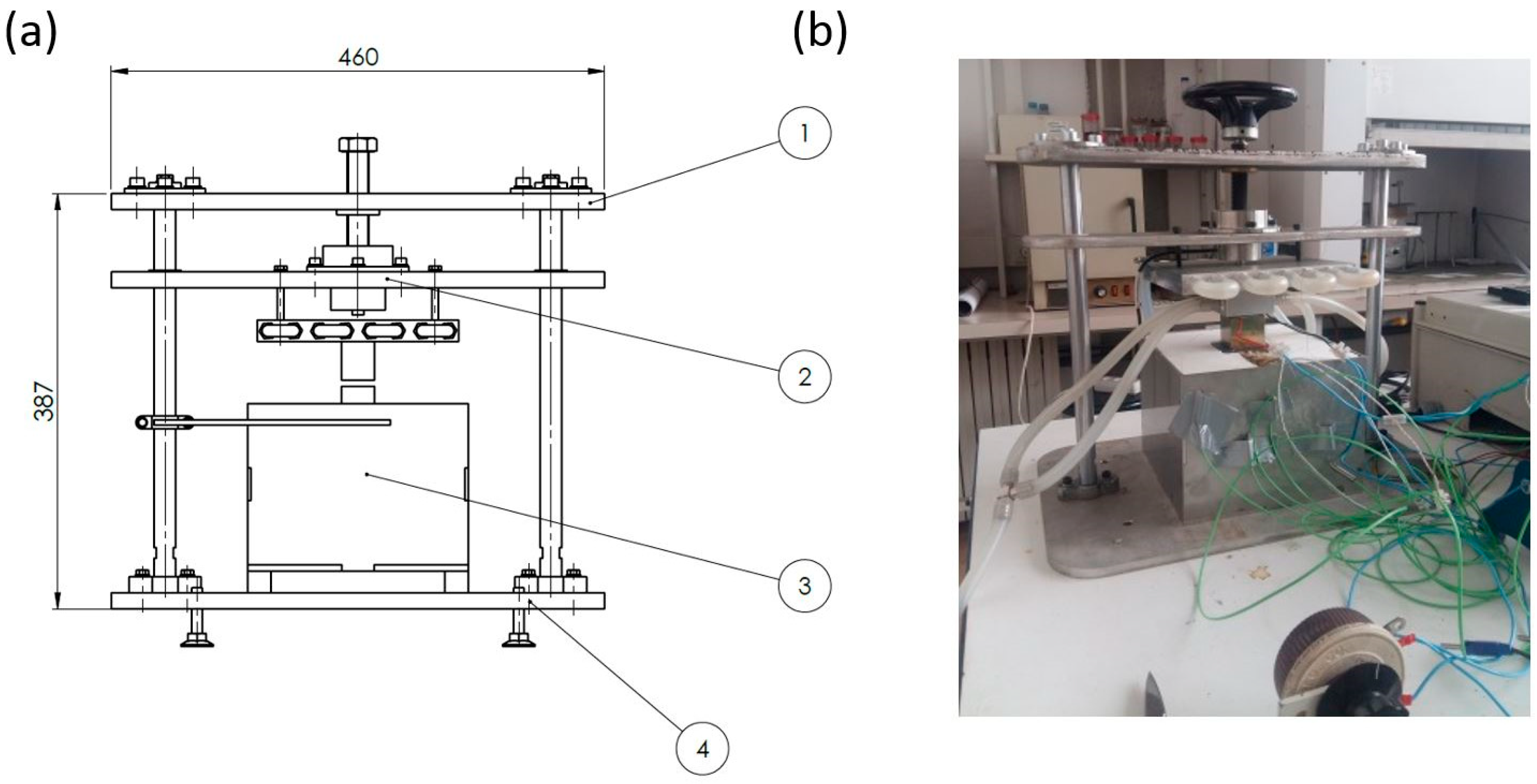
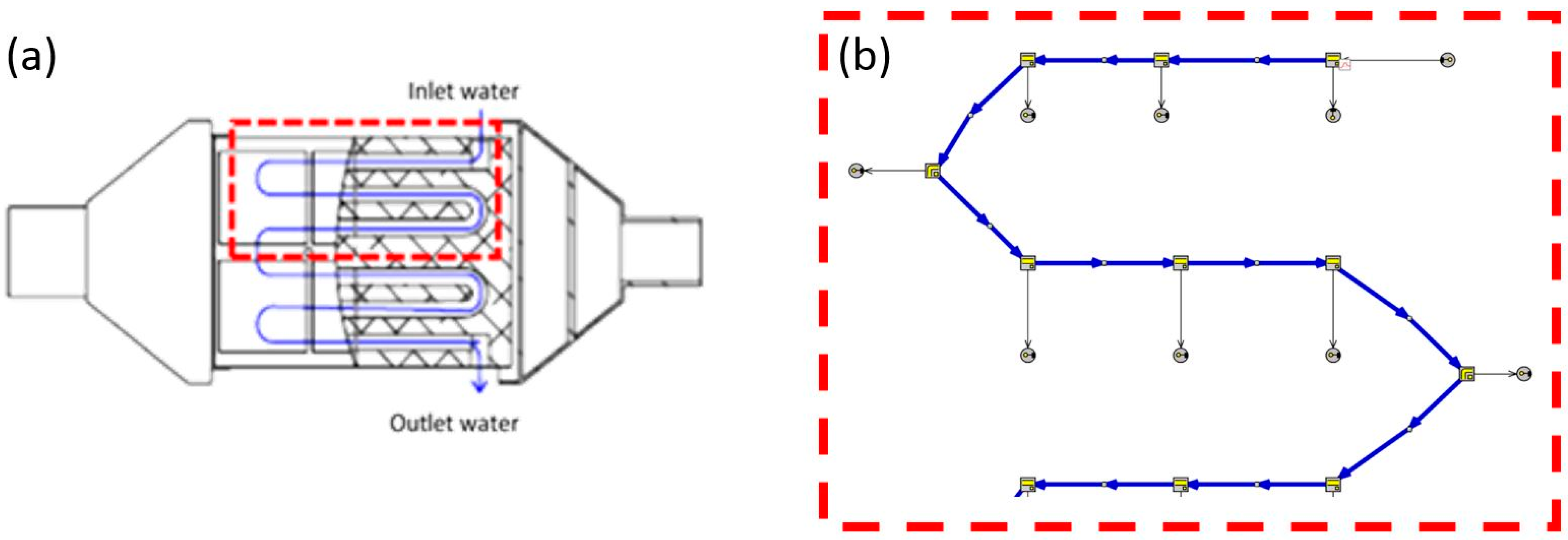
3.1. Automotive Thermoelectric Generator

The ATEG employed in our study was previously tested in experimental studies with a spark ignition engine under stationary [18] and normalized driving cycle conditions [5]. These previous studies led to the development of an analytical method to assess the variation in fuel consumption when an ATEG is installed in a vehicle [18]. However, the ATEG used in References [5,18] might have been working in far from optimum conditions since there was no information on how changes to its key design parameters would affect its performance. Therefore, our objective was to validate a numerical model of the ATEG to improve its design by investigating the consequences of varying the most relevant design parameters, as described next.

The heat absorber or hot-side heat exchanger (HSHE) of this ATEG consisted of a 210 × 140 × 15 mm (length × width × height) copper plate with six cylindrical holes 12 mm in diameter (#1 in Figure 1a). A total of 12 commercial TEMs (TELBP1-12656-0.45, Thermonamic Electronics Corp., Ltd., Nanchang, China)—six TEMs each for the upper and lower faces of the heat absorber (#2 in Figure 1a)—were installed in the ATEG. On each face, the six TEMs were distributed in two rows (aligned with the direction of the exhaust gases) and three columns (perpendicular to the direction of the exhaust gases). The dimensions of a single TEM were 56 × 56 mm (length × width) with a total surface area of A_TEM = 3136 mm² and total height of L_TEM = 5 mm. Each TEM was formed by 116 small legs of thermoelectric material (PbTe and BiTe based). These TEMs can cope with hot-side temperatures of 360 °C and, occasionally, of 400 °C.

The cold side of the TEMs was in contact with an aluminum block or cold-side heat exchanger (CSHE; #3 in Figure 1a), that acted as a heat sink since water flowed in a wavy path within it (Figure 1b). The rectangular cross-sectional area of the water channel was 12 × 10 mm (height × width). Both the upper and lower cooling blocks were clamped together to provide the pressure required on the faces of the TEMs (1.27 MPa). Since the TEMs used a graphite sheet on both the cold and hot sides, no additional thermal interface material was required to improve heat transfer.

The HSHE was connected to the circular cross-sectional area of the exhaust pipes (50 mm in diameter) by expansion and contraction elements (#4 in Figure 1a) very similar to those employed in other types of ATEGs whose designs are based on TEMs located on two parallel plates (e.g., References [6,13,15]). The overall dimensions of the ATEG were 440 × 200 × 20 mm (length × width × height) and a total weight of 7 kg. The electrical connection of all the TEMs was in series as this was expected to provide higher electrical power output than in parallel [35]. The effect of using electrical hybrid connections was not analyzed here.

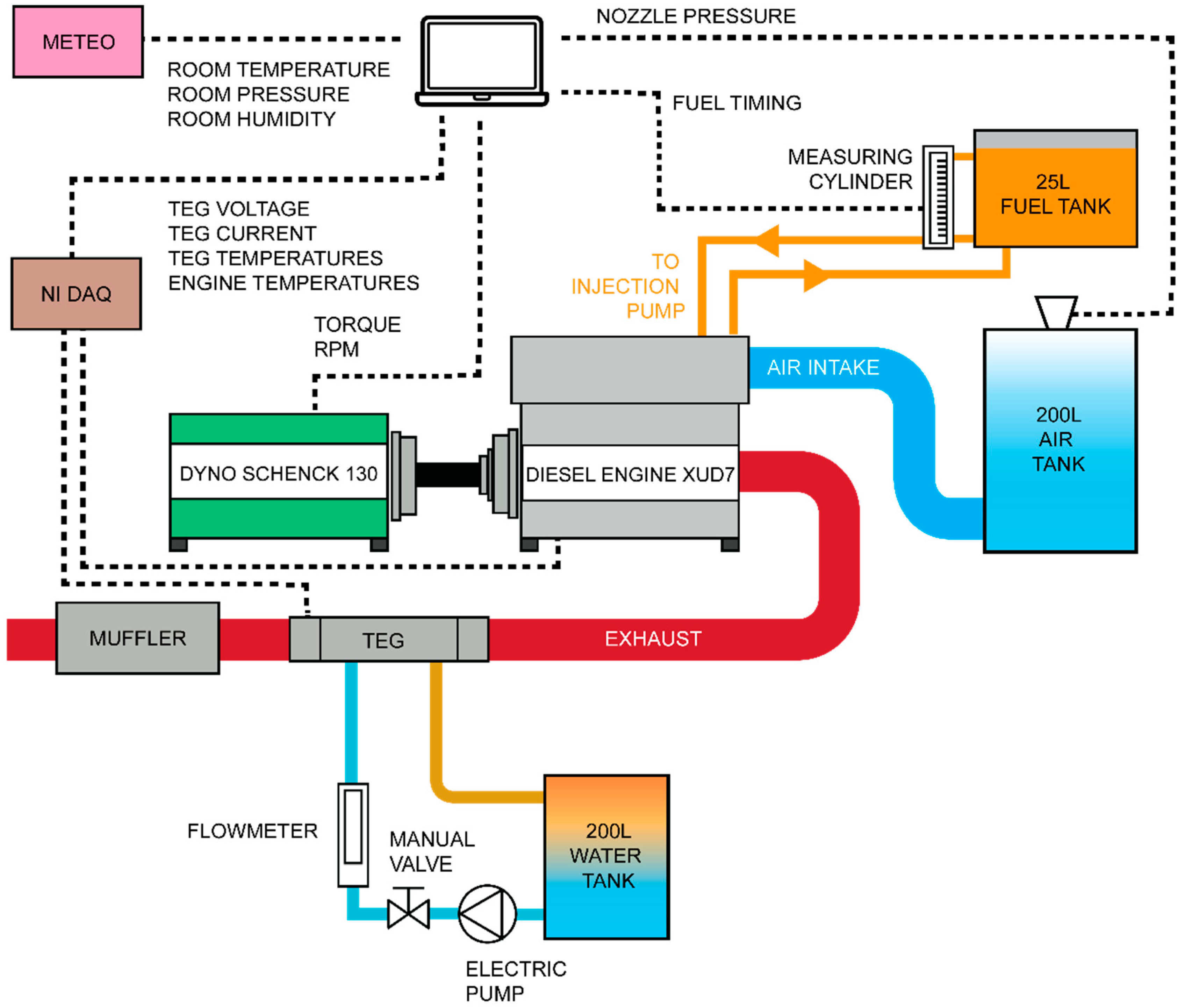
3.2. Experimental Set-Up

We used the same experimental set-up employed by Reference [35], who analyzed an ATEG formed by a single TEM. In essence, a PSA XUD7 version K (Peugeot S.A., Rueil-Malmaison, France) (an in-line four-cylinder 1.8-L naturally aspirated diesel engine of 44 kW of nominal power) was connected to a Schenck W130 dynamometer (Figure 2). The ATEG was installed very close to the exhaust manifold and in front of the muffler to ensure high temperature gases at the ATEG inlet (Figure 3). The engine coolant temperature was between 80 °C and 90 °C under regular functioning. The high temperature employed as a cooling flow in the CSHE would substantially reduce the performance of the ATEG. Therefore, to cool the ATEG we designed an independent closed-circuit water system with a 200-L tank and an electric pump. The range of flow rates varied from 140 to 580 L/h depending on the case tested. The series electrical configuration of the TEMs was connected to a variable external load resistance in order to attain the maximum output power.

We monitored the following information: engine torque, engine speed (rpm), exhaust mass flow rate, exhaust gas temperature at both ATEG inlet and outlet, water cooling volumetric flow rate, water cooling temperatures at both ATEG inlet and outlet, ambient temperature, ATEG output voltage, and output current (see Figure 2).

Temperatures were measured with type-K thermocouples using a National Instruments (NI) Compact RIO system with 9211 modules. Electrical information was also measured by an NI Compact RIO with 9215 (voltage) and 9227 (current) modules. Data were processed with LabVIEW software (version 2016, National Instruments, Austin, TX, USA). Engine torque, speed, and temperature were monitored with a Sportdevices SP4 unit. The mass flow rate of exhaust gases was calculated as the sum of the mass flow of air at the intake manifold plus the mass flow of consumed fuel. The volumetric flow rate of air at the inlet of the engine was measured with a calibrated Tecner TG40 nozzle installed at the inlet of a 200-L-capacity tank that damped the pulsating signal of the engine intake. The conversion of volumetric flow rate to mass flow rate used the air density calculated with the ideal gas law. At each stationary regime, the mass flow rate of fuel was obtained after measuring the time span needed to consume 30 cm³ of net fuel (injected minus returned) in a calibrated measuring cylinder. The variation of fuel density with temperature was previously obtained with a thermostatic bath at different temperatures and a densimeter.

The experimental uncertainty and the accuracy of the equipment used in the experimental tests followed the procedure detailed in Reference [35]. In essence, we assumed that the total uncertainty of a measured variable was the sum of an uncertainty related to the recorded time series plus an uncertainty related to the accuracy of the equipment.

Once the system reached stationary conditions, data were acquired during a time interval of 60 s minimum. Averaged values of the variables measured for these time series were calculated, and the uncertainty related to the mean values ${\epsilon }_s$ was expressed as

$${\epsilon }_s=\pm z_{\alpha /2}\frac{\sigma }{\sqrt{N}},$$

(1)

where $z_{\alpha /2}$ was the confidence range (here chosen as 95%), σ was the standard deviation of the data series, and N was the number of samples in the data series.

On the other hand, the uncertainty of the equipment ${\epsilon }_e$ was obtained from

$${\epsilon }_e={\displaystyle \sum }\left|\frac{\partial Y}{\partial x}\right|\mathsf{\Delta }x,$$

(2)

where $Y$ corresponded to the indirect variable, $x$ referred to the direct measured variable, and $\mathsf{\Delta }x$ was the accuracy of the equipment in the measurement of the $x$ variable.

Thus, the total uncertainty of data ${\epsilon }_t$ followed

$${\epsilon }_t=\sqrt{{\epsilon }_s^2+{\epsilon }_e^2}.$$

(3)

The accuracy of the experimental equipment is listed in

Table 2. Accuracy of the experimental equipment. NI—National Instruments.

Equipment	Accuracy	Ref.
Current (NI 9227)	± (169.7 mA + 5% of reading)	[36]
Voltage (NI 9215)	± (85.3 mV + 1.05% of reading)	[36]
Temperature (NI 9211)	± 0.6 °C	[36]
Type K thermocouple	± 1.5 °C	[37]
Sensus 405 S water meter	± 0.05 L	[38]
Manometer	± 10 Pa
Fuel Calibrated volume cylinder	± 0.5 cm3

.

3.3. Experimental Cases

Seven different engine operating points were investigated (see

Table 3. Experimental data for engine regime, torque, exhaust gas mass flow rate ${\dot{m}}_g$, exhaust gas temperature at ATEG inlet T_g,i, water cooling volumetric flow rate ${\dot{V}}_w$, water coolant temperature at ATEG inlet T_w,i and air–fuel equivalence ratio λ.

Case	Regime (rpm)	Torque (N·m)	${\dot{\mathit{m}}}_{\mathit{g}}$ (g/s)	Tg,i (°C)	${\dot{\mathit{V}}}_{\mathit{w}}$ (L/h)	Tw,i (°C)	λ
1	2500	69.9 ± 0.1	43.4 ± 0.3	444.7 ± 2.0	580 ± 3	26.4 ± 2.0	1.68
2	2500	67.3 ± 0.1	42.8 ± 0.3	428.7 ± 2.0	280 ± 3	31.2 ± 2.0	1.68
3	2500	71.9 ± 0.1	43.0 ± 0.3	450.1 ± 2.1	160 ± 3	33.6 ± 2.0	1.63
4	2800	75.1 ± 0.1	46.1 ± 0.3	521.6 ± 2.1	580 ± 3	29.6 ± 2.0	1.50
5	2600	82.2 ± 0.1	44.4 ± 0.3	547.4 ± 2.0	140 ± 3	33.4 ± 2.0	1.43
6	3000	79.2 ± 0.1	48.3 ± 0.3	598.8 ± 2.0	580 ± 3	28.0 ± 2.0	1.34
7	3200	76.1 ± 0.1	51.0 ± 0.3	598.5 ± 2.0	180 ± 3	34.5 ± 2.0	1.36

). These points were chosen according to the purpose of the present research, i.e., to investigate the effects of changing the main geometrical parameters of the ATEG and, also, the volumetric flow rate of the ATEG coolant (${\dot{V}}_w$). Since we tested a single ATEG, the objective was to experimentally obtain points varying the flow rate of the cooling water at different engine-shaft power P_e values. Thus, cases 1 to 3 corresponded to P_e ≈ 18 kW with different values of ${\dot{V}}_w$, ranging from the maximum (580 L/h) to almost the minimum (160 L/h). Cases 4 to 5 had P_e ≈ 22 kW and ${\dot{V}}_w$ ranging from 580 L/h to 140 L/h, respectively. Finally, cases 6 to 7 had P_e ≈ 25 kW and ${\dot{V}}_w$ ranging from 580 L/h to 180 L/h, respectively. Cases with P_e values lower than 18 kW were not tested since they were expected to provide low electrical output power [18]. Values of flow rate and temperature at the inlet of the ATEG for both the exhaust gases and coolant water, as well as air–fuel ratio, were later used as boundary conditions at the inlet of the ATEG in the numerical model. For each one of the seven different engine operating points, the external electrical resistance was tuned to achieve the maximum output power.

3.4. Effective Thermal and Electrial Properties of the Thermoelectric Modules

The numerical model described in Section 4 adopted the strategy of interpreting each TEM as a single body with effective thermal and electrical properties. Therefore, we required the values of the effective Seebeck coefficient, the effective internal resistance, and the effective thermal conductivity. These effective properties were obtained with the test rig of thermoelectric modules that is schematically shown in Figure 4a.

In essence, the test rig consisted of a 400-W cartridge heater inserted into a 56 × 56 × 30 mm (length × width × height) bronze rectangular prism that was immersed inside a 200 × 200 × 150 mm (length × width × height) block filled with sheets of calcium silicate (#3 in Figure 4a). This thermal-insulating material has a thermal conductivity of only 0.072 W·m⁻¹·K⁻¹ at 200 °C and guarantees thermal stability up to 1000 °C. An additional 56 × 56 × 36 mm (length × width × height) rectangular bronze prism was placed on the top side of the bronze heated by the cartridge. This supplementary bronze block acted to delimit the path of the heat flow. The thermal conductivity of this block was k_b = 86.5 W·m⁻¹·K⁻¹ (C54400 85% Cu, 5% Sn, 5% Pb, 5% Zn composition). In this block, we inserted two K-type thermocouples vertically separated by a distance L_b = 30 mm. Since the lateral sides of this block were in contact with thermal-insulating sheets of calcium silicate, we approximated the vertical heat flow Q_h through this element as

$$Q_h=\frac{k_b{A}_b T_b}{L_b},$$

(4)

where A_b (= 56 × 56 mm) was the cross-sectional area of the block, and $\mathsf{\Delta }{T}_b$ was the temperature difference between the two abovementioned thermocouples.

The upper face of the bronze block was in contact with the hot side of the TEM being tested (see Figure 4a,b). The cold side of the TEM was in contact with a 56 × 56 × 30 mm (length × width × height) aluminum block. The upper side of this aluminum block was, at the same time, in contact with a water heat exchanger. This heat sink was pressed against the TEM with a vertical screw (Figure 4a). A load cell (LCM305, Omega Engineering Ltd; #2 in Figure 4a) measured the force applied. Frame elements, including the vertical guide bars (#1 in Figure 4a) and the base plate (#4 in Figure 4a), were made of stainless steel.

The hot- (T_h) and cold-side (T_c) temperatures of the TEM were measured with thin K-type thermocouples 0.2 mm in diameter and located between the upper face of the supplementary bronze element and the TEM’s hot side, and between the lower face of the aluminum block and the TEM’s cold side, respectively. To ensure a uniform contact between surfaces, thermocouples were inserted in slits made of 0.2-mm-thick brass sheets with a 56 × 56 mm cross-sectional area.

The TEM was electrically connected to an external variable resistance. Voltage and current were acquired with the same instruments as those described in Section 3.2. Results were obtained for a load pressure equal to 1.27 MPa in ambient conditions (equivalent to 3983 N force and equal to that applied in the ATEG) and a T_h temperature range from 140 °C to 226 °C and for T_c from 38 °C to 70 °C, expected to be similar to those obtained in the ATEG once installed in the engine test bench. Maximum electrical output power data were reported by suitably tuning the value of the external load resistance.

From the data obtained with the test rig, the effective Seebeck coefficient ${\alpha }_e$ of the TEM was calculated as

$${\alpha }_e=\frac{V_{oc}}{T_h-T_c},$$

(5)

where V_oc was the open-circuit voltage.

On the other hand, the effective thermal conductivity $k_e$ of the TEM was calculated as

$$k_e=\frac{L_{TEM} Q_h}{A_{TEM}\left(T_h-T_c\right)},$$

(6)

where L_TEM (= 5 mm) was the total height of the TEM, and A_TEM (= 3136 mm²) was its cross-sectional area.

Finally, the effective internal electrical resistance $R_{ie}$ was calculated as

$$R_{ie}=\frac{V_{oc}-I_{TEM} R_L}{I_{TEM}},$$

(7)

where $I_{TEM}$ was the electrical current of the TEM when the external load resistance was $R_L$.

4. Numerical Model

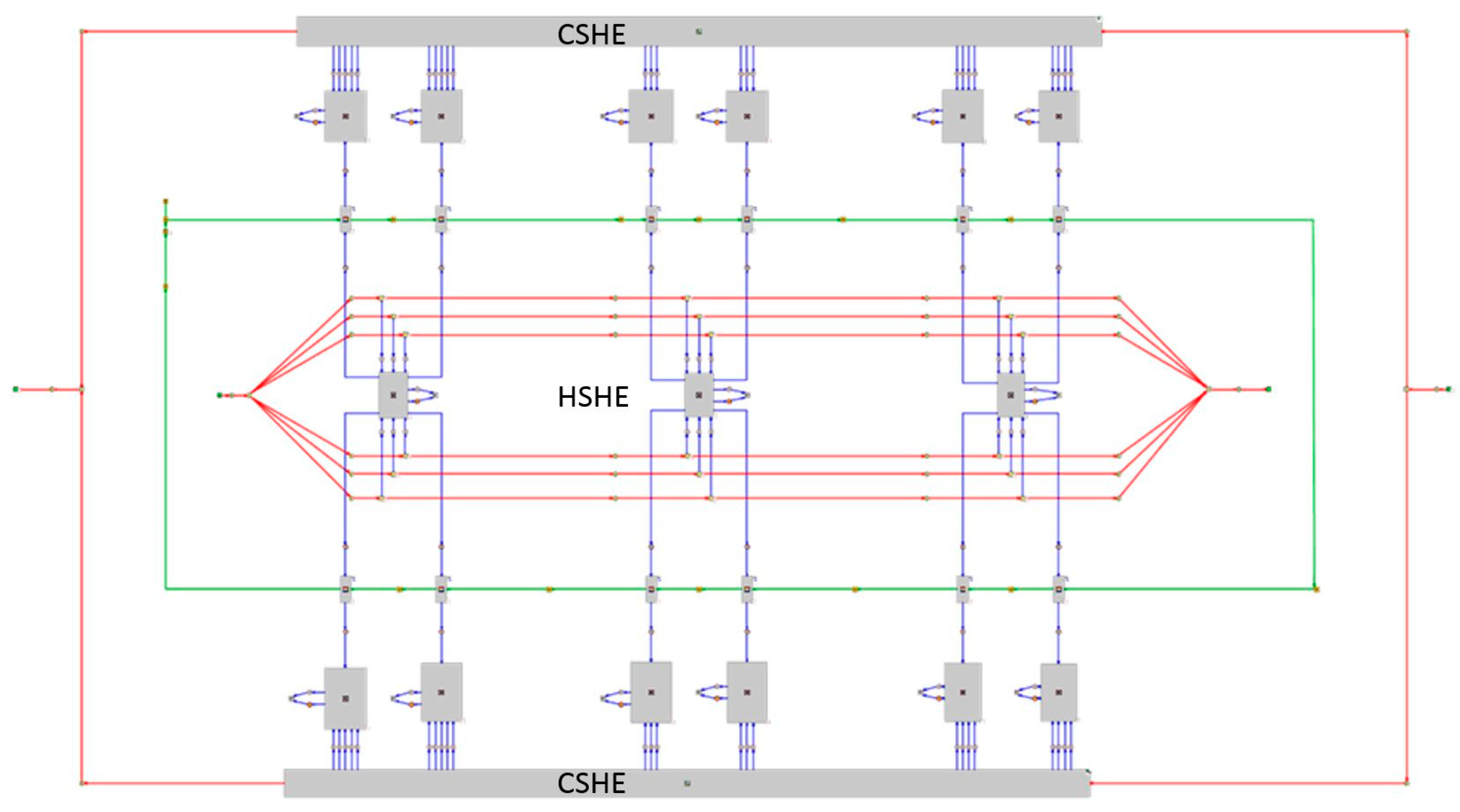
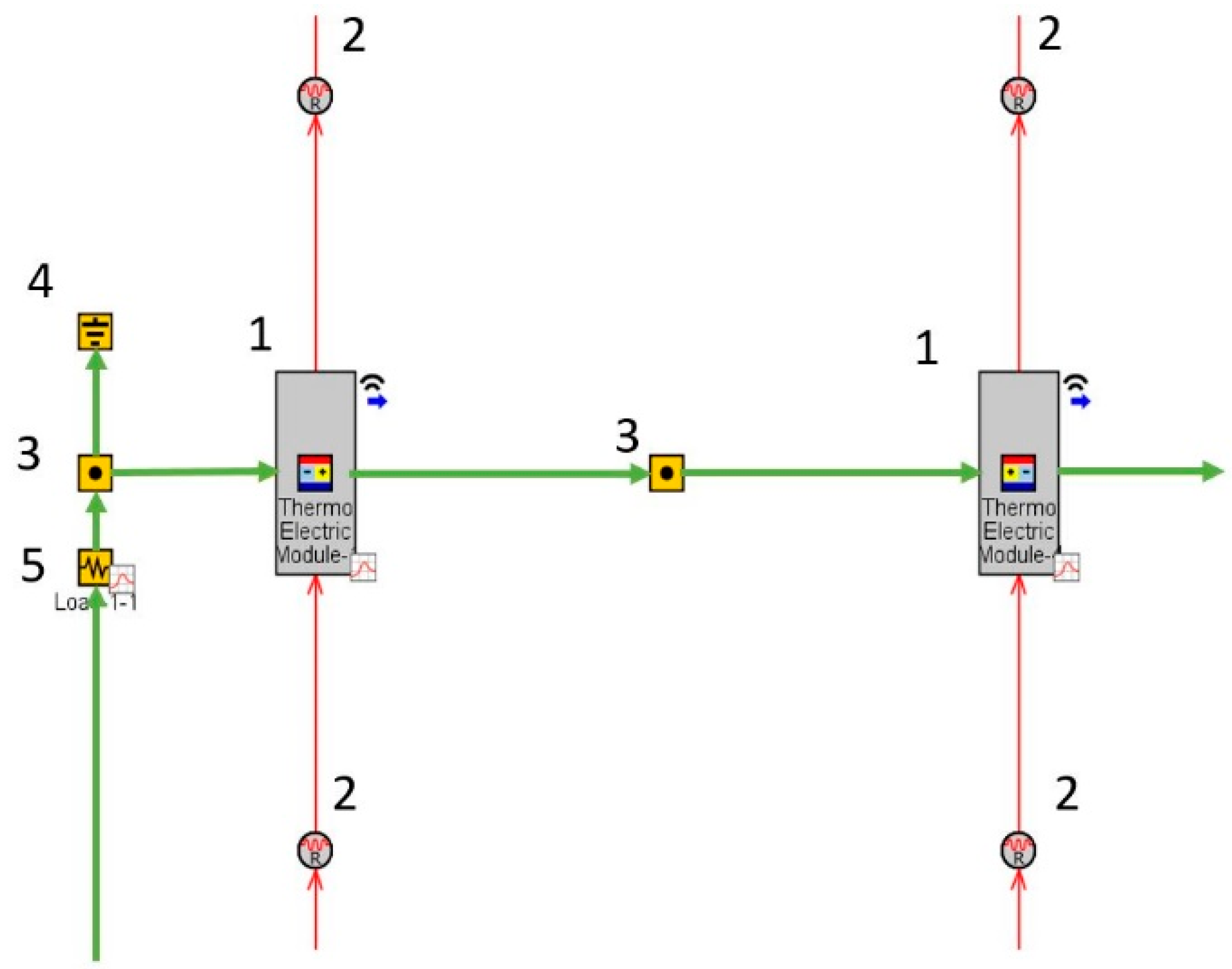
4.1. Simulation Set-Up

Simulations were performed using the GT-SUITE software, which is a multi-physics CAE system widely used in the automotive sector [34]. GT-SUITE is composed of a set of libraries whose combination allows fluid flows and their interactions with solid bodies, including heat transfer mechanisms, to be simulated. This software was used to study the behavior of exhaust gases in ICEs, analyzing, for example, the effects the exhaust gas recirculation system has on internal combustion engines [39], and investigating waste heat recovery technologies such as the Organic Rankine Cycle [40], turbocompounding [41], and ATEGs [35].

GT-SUITE’s modeling methodology is based on linking several submodels, each one focused on solving a specific problem. Figure 5 shows the schematic diagram of the whole model developed to reproduce our ATEG.

The copper heat exchanger was divided into three thermal masses connected in series. Thus, each thermal mass corresponded to the part of the heat exchanger assigned to the four TEMs located in the same column (see Figure 1). This method of segmenting the hot heat exchanger along the exhaust flow direction allowed us to correctly simulate the disparity of cold- and hot-side temperatures among TEMs, one of the main drawbacks observed in ATEG designs. The surfaces of these thermal masses were appropriately connected to (1) the exhaust gases through six cylindrical surfaces, (2) the hot sides of TEMs, and (3) the ambient (see Figure 6). Heat transfer via conduction and convection was assumed and the external surface (contact with the environment) used a heat transfer coefficient h = 25 W·m⁻²·K⁻¹ [42]. It also included losses via radiation with a gray body emissivity of the thermal mass surface equal to 0.9. The Colburn analogy was used for heat transfer via convection in fluids [42].

TEMs were modeled by assuming them to be uniform bodies with the effective thermal and electrical properties obtained in Section 3.4. Thus, we avoided the task of simulating each and every thermoelement that formed the TEM. The hot side of each TEM was in contact with the corresponding thermal mass of the copper heat absorber or HSHE, whereas the cold side was in contact with the water heat sink or CSHE (Figure 7). The thermal connection between thermal masses and the TEMs’ hot side and between water heat sink and the TEMs’ cold side applied constant values for the thermal contact resistances R_h and R_c, respectively. These values were chosen as R_h = 5 × 10⁻⁴ m²·K·W⁻¹ and R_c = 3 × 10⁻⁴ m²·K·W⁻¹ in agreement with those used in similar ATEGs [5]. Changes of R_h and R_c with respect to temperature were not expected to substantially vary the results, as concluded in Reference [35], nor would they alter the conclusions of the present study.

The cold side of each TEM was in contact with heat sink zones corresponding to different water paths (see Figure 8a). To model this effect, we divided the heat sink into 24 sections depending on their location with respect to the TEMs below. Each one of these sections was thermally connected to the corresponding region of the aluminum heat sink that, at the same time, was thermally connected to the cold side of the pertaining TEM (adding a thermal contact resistance R_c as mentioned previously; see Figure 8b).

To correctly reproduce the experimental conditions, simulations used water as the coolant and the product of a combustion reaction as the exhaust gases. The latter assumption better represented actual laboratory conditions than imposing air as exhaust gases, as commonly adopted in other numerical models of ATEGs [7,18]. A complete combustion reaction of diesel fuel with an air–fuel ratio (AFR) higher than that of stoichiometric conditions (AFR_s) was implemented and properties such as dynamical viscosity, thermal conductivity, specific heat, etc., as a function of the temperature of the mixed gas were used in the calculations. The actual air–fuel equivalence ratio values (λ = AFR/AFR_s) for each experimental point were deduced from measurements, giving lean conditions (λ > 1) in all of the engine operation points analyzed (see Table 3).

The electrical behavior of the ATEG was also simulated with GT-SUITE by electrically connecting all TEMs in a series configuration to an external electrical load resistance R_L. Effective values of the Seebeck coefficient, the thermal conductivity, and the internal resistance of each TEM followed those obtained in Section 3.4, and are listed in

Table 4. Effective values of Seebeck coefficient (α_e), thermal conductivity (k_e), internal electrical resistance (R_ei), and figure of merit (ZT_e) as a function of cold- (T_c) and hot-side (T_h) TEM temperatures.

Tc (°C)	Th (°C)	αe (V·K−1)	ke (W·m−1·K−1)	Rei (Ω)	$\mathit{Z}{\mathit{T}}_{\mathit{e}}$
38	140	0.0255	3.17	0.759	0.157
39	160	0.0263	2.94	0.781	0.180
42	180	0.0272	2.90	0.814	0.192
50	160	0.0267	3.00	0.806	0.179
51	170	0.0274	3.02	0.838	0.183
55	181	0.0280	2.97	0.829	0.199
55	201	0.0280	2.84	0.834	0.212
65	201	0.0279	2.87	0.787	0.214
65	226	0.0296	2.73	0.922	0.232
70	140	0.0261	3.15	0.729	0.179
70	160	0.0267	3.11	0.760	0.186

. The effective figure of merit was calculated as $Z{T}_e={\alpha }_e^2\overline{T}/\left({\rho }_e{k}_e\right)$ where $\overline{T}=\left(T_h+T_c\right)/2$ and the effective electrical resistivity ${\rho }_e=A_{TEM}{R}_{ei}/L_{TEM}$. $Z{T}_e$ was obtained for illustrative purposes only since the model did not require this value.

The thermal and the electrical effective properties of each TEM as a function of temperature were determined by extrapolating the data of Table 4. This mathematical procedure was carried out by the GT-SUITE software, in which data were introduced in tabular form. Thermal properties of aluminum and copper as a function of temperature were taken into account using the own engineering libraries of the software.

The model took into account the coupling between the thermal and the electrical phenomena. Thus, the heat flow on the cold side of the TEM, $Q_{\mathrm{c}}$, corresponded to that on the hot side, $Q_h$, minus the generated electrical power$P_{TEM}$:

$$Q_c=Q_h-P_{TEM},$$

(8)

and both the cold and hot heat flows were calculated as

$$Q_c={\alpha }_e I_{TEM}{T}_c+\frac{k_e A_{TEM}}{L_{TEM}}\left(T_h-T_c\right)-\frac{1}{2}{I}_{TEM}^2{R}_{ie},$$

(9)

$$Q_h={\alpha }_e I_{TEM}{T}_h+\frac{k_e A_{TEM}}{L_{TEM}}\left(T_h-T_c\right)+\frac{1}{2}{I}_{TEM}^2{R}_{ie},$$

(10)

where I_TEM was the current flowing through the TEM, and was the same as that of the whole ATEG since the electrical connections were in pure series. The sum of the electrical power of all individual TEMs gave the total power generated by the ATEG P_ATEG.

In Equations (9) and (10), the first term corresponds to the Seebeck contribution (i.e., the thermoelectric effect), the second to Fourier’s law, and the last to Joule heating. The Thomson effect was neglected since its contribution was expected to be of minor importance in comparison to the other three terms [35].

The global boundary conditions of the simulation were the following: exhaust gas at ATEG inlet, fixed temperature and mass flow rate (see Table 3); exhaust gas at ATEG outlet, fixed pressure (set to the atmospheric one); cooling water at ATEG inlet, fixed temperature and volumetric flow rate of cooling water (Table 3); cooling water at ATEG outlet, fixed pressure (set to the atmospheric one); fixed ambient temperature at 24 °C. The value of the external electrical load resistance was tuned to maximize a goal function (in this case, the electrical output power of the ATEG to validate the model). The optimization procedure is explained in Reference [35].

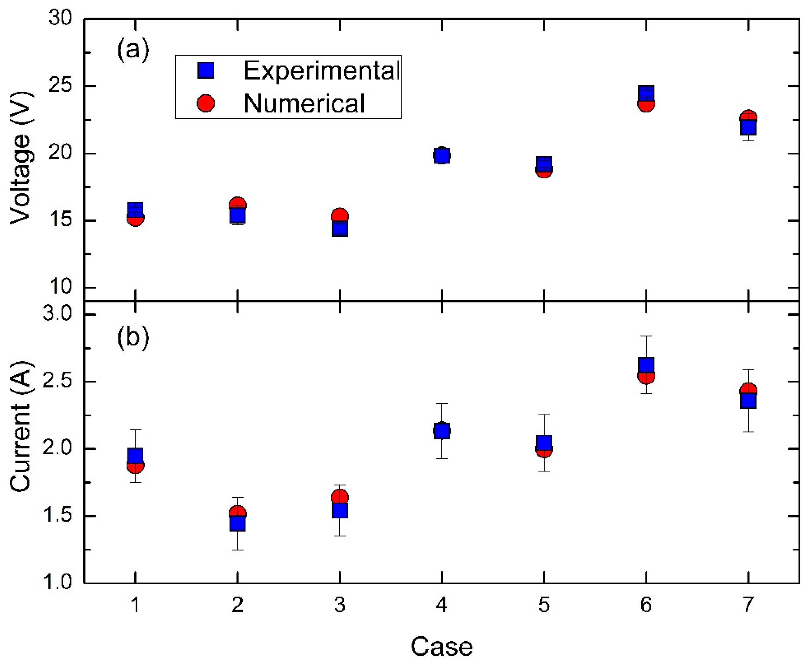
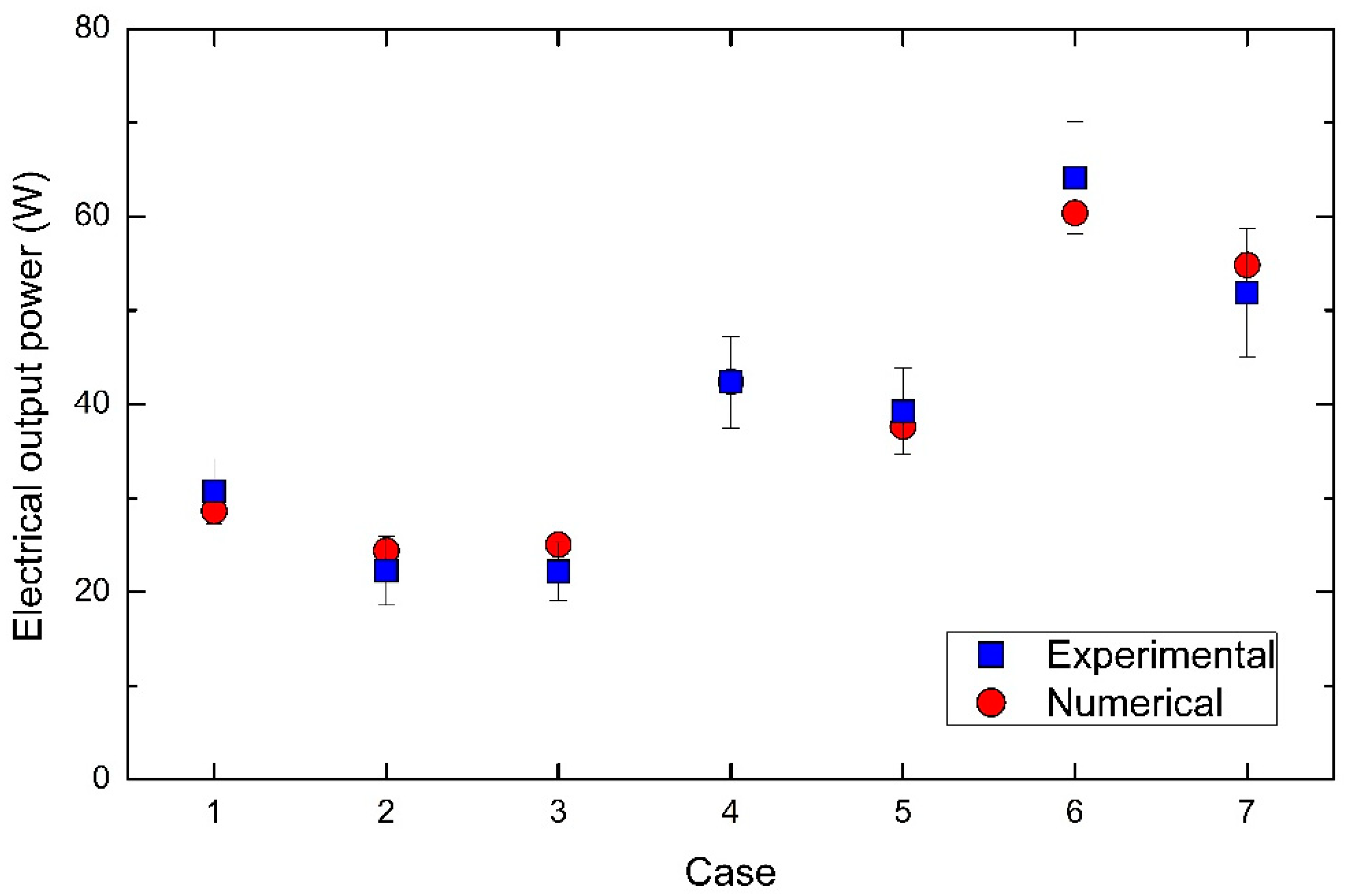
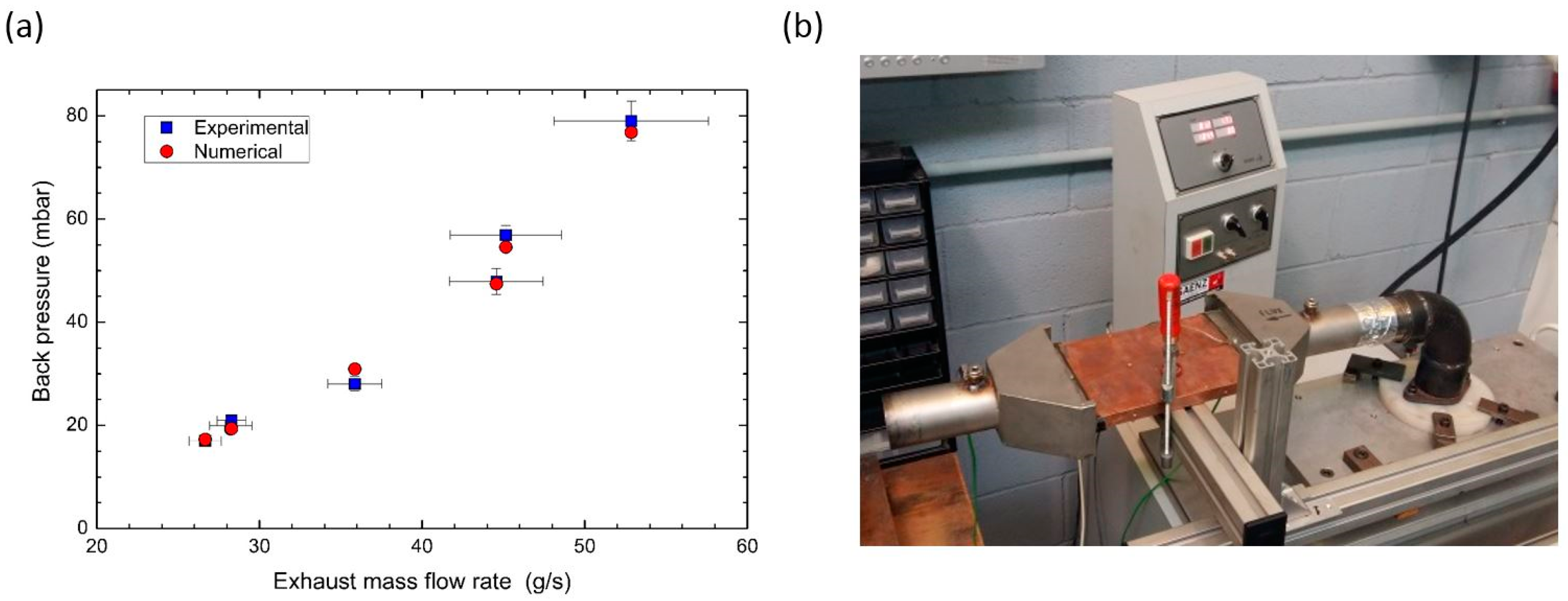
4.2. Model Validation

The results from the model were compared with the experimentally measured values. For the thermal behavior, the prediction of the temperature at the outlet of both fluid flows (exhaust gas and water cooling) is shown in Figure 9. Simulation results coincided with the experimental values (within their uncertainty ranges) with small discrepancies only in the water outlet temperature for cases 5 (<1.5%) and 7 (<5%). The agreement of the simulations with the exhaust gas temperature measured at the ATEG outlet was quite remarkable since the experimental cases covered a broad range of values (i.e., gas temperature at ATEG inlet from 428 °C to 599 °C). Therefore, the results indicated that the model correctly predicted the heat transfer in the ATEG (i.e., from the exhaust gas to the water cooling).

The conversion of heat into electricity by the TEMs’ effective properties mentioned above also reproduced very well the electrical values obtained experimentally (Figure 10). The simulated voltage and current values matched the laboratory data within their uncertainty ranges. Note that the highest voltage values (>23 V) were obtained at very demanding engine speeds. The agreement of the results with the measured data confirmed the validity of the methodology implemented for determining the external resistance load that would maximize the output power.

The electrical output power of the whole ATEG P_ATEG simulated by GT-SUITE for the cases listed in Table 3 were compared with the experimental ones (Figure 11). Case 6 obtained the maximum power value, reaching up to 64 W. This meant an average power production per TEM equal to 5.3 W. Since voltage and current were already well predicted by the model, simulated output power production followed the values observed. The trend obtained in the experimental cases was also replicated by the model.

Thus, we accepted that our methodology correctly predicted the behavior of our ATEG (in both the thermal and electrical behavior). That said, in fuel consumption analysis, it is critical to correctly determine the energy losses through the ATEG. Indeed, the increase in the upstream pressure once the ATEG is installed in the exhaust (or, equivalently, the head losses experienced by the exhaust gas when moving through the ATEG) becomes one of the main ATEG design parameters [6,10,13]. These head losses can be directly related to the back pressure, which is defined as the pressure difference between the ATEG inlet (upstream, high pressure) and the ATEG outlet (downstream, low pressure).

Thus, an additional validation was required if the model were to be used as a tool to investigate the effect the ATEG has on fuel consumption. Due to laboratory limitations, pressure differences through the ATEG could not be measured on the engine test bench. However, back pressure values were experimentally obtained when the ATEG was disassembled from the exhaust pipe and installed in a flow bench (Saenz D640). Seven different amounts of air mass flow rates and air temperatures were pumped through, and the results of the back pressure values were recorded (Figure 12). Simulations of the ATEG were carried out without a cooling system, but with the ATEG conditions at the inlet of the exhaust pipe the same as those applied in the flow bench. Results also matched the measured values within their uncertainty ranges, which implied that the flow dynamics of the exhaust gas in terms of energy losses (i.e., back pressure) were also being correctly simulated by the model (Figure 12a).

5. Results and Discussion

Our objective was to investigate the performance of our ATEG (output power and fuel economy) having changed the main design parameters of its heat exchangers (HSHE and CSHE). For a fixed distribution of TEMs (i.e., 12 TEMs and specified values for the temperature and mass flow rate of the exhaust gases), the main design parameter of the HSHE is the diameter of the cylindrical holes (D), since length is determined by the dimensions of the TEMs. On the other hand, the main design parameters for the CSHE are the volumetric flow rate of cooling water and the value of the cross-sectional area of the water channel. The consequences of modifying these parameters are shown next.

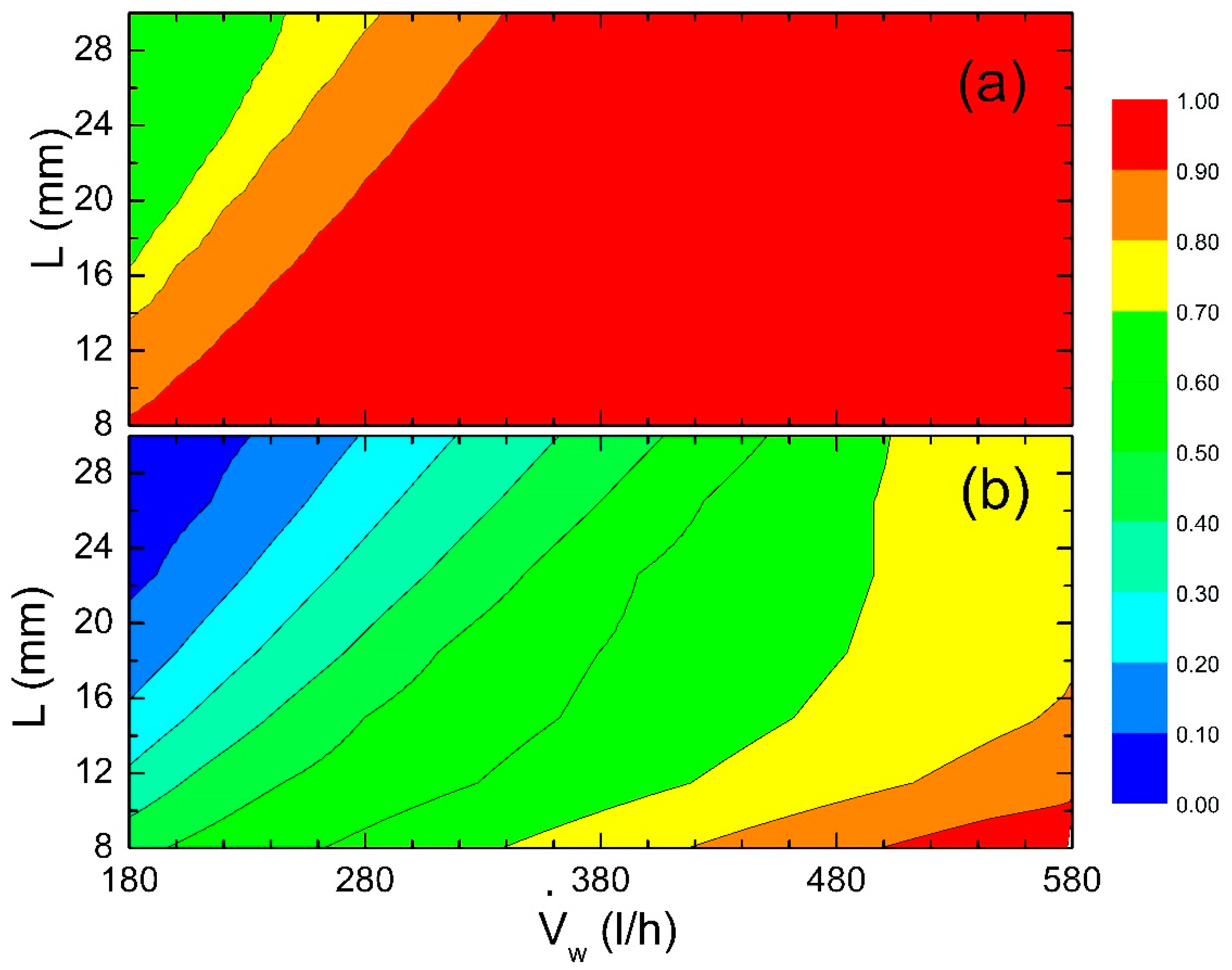
5.1. Water Heat Sink: Effects of Changing the Geometry and Flow Rate

The height of the cooling channel L in the water heat sink was varied from 8 mm to 30 mm while the width (= 10 mm) was kept constant. This meant a variation from 80 mm² to 300 mm² in the cross-sectional area of the water channel. We also investigated the effects of changing the volumetric flow rate of the cooling water, ${\dot{V}}_w$, varying it from 140 L/h up to 580 L/h. This represented an average water velocity within the channel ranging from 0.13 m/s (case with ${\dot{V}}_w$ = 140 L/h and L = 30 mm) to 2.01 m/s (case with ${\dot{V}}_w$ = 580 L/h and L = 8 mm). Note that not all the combinations of ${\dot{V}}_w$ and L implied turbulent conditions. However, being based on the Colburn analogy, the calculations for the convective heat transfer assumed different equations depending on the flow regime (see Reference [42]).

Simulations for L ranged between 8 and 30 mm with 1-mm increments and, for ${\dot{V}}_w$, they ranged between 140 and 580 L/h with 20-L/h increments taking the boundary conditions of the maximum output power case achieved in the experimental test (case 6 in Table 3 but with a variable ${\dot{V}}_w$). For each one of the configurations (L and ${\dot{V}}_w$) simulated, the model applied a numerical algorithm to find the maximum output power by suitably varying the external load resistance, R_L. In Figure 13, the degree of intensity of the convective heat transfer between the heat sink’s aluminum block and the cooling water flowing in its interior was analyzed by calculating the convective heat transfer coefficient, h, and the area of the aluminum channel in contact with the water, A. This hA product (which is, indeed, the inverse of the thermal resistance) was evaluated by taking h as the value calculated at the end of the water channel path. Results shown in Figure 13b confirmed that the maximum heat transfer was achieved with the maximum flow rate and minimum height, thereby maximizing the flow velocity. Although hA substantially varied in the range of flow rates and water channel heights analyzed, its influence on the maximum electrical power extracted from the exhaust gases (Figure 13a) was not important until its value was below 2.70 W·K⁻¹ (thermal resistance equal to 0.37 K·W⁻¹; electrical output power of 57.5 W in comparison with the maximum obtained of 63.9 W). The CSHE had a remarkable impact on the reduction in output power as hA further decreased (at low flow rates and high cross-sectional areas of the water channel) and, consequently, the thermal resistance increased. A similar behavior was observed in Reference [43] when the behavior of a TEG designed for a different purpose (it used hot water instead of exhaust gases as the main heat source) was experimentally studied.

While the results above focused on the power output, the final target of installing an ATEG in a vehicle is in fact to reduce fuel consumption. The P_ATEG value generated charges the battery of the vehicle. As previously mentioned, this reduces the time demand on the vehicle’s electrical generator (i.e., the alternator) and, consequently, increases fuel economy. Nevertheless, because of the effect of the back pressure, due to the pressure increase upstream, the ATEG increases fuel consumption with respect to the pristine conditions of the vehicle. In addition, the ATEG has a non-negligible mass that should be added to the total mass of the vehicle. This weight increase also leads to increases in fuel consumption.

The impact of these three effects on fuel efficiency were estimated by Karri et al. [19], who proposed the following equations to estimate fuel economy resulting from the power generated by the ATEG ($F_{e,ATEG}$), the increase in fuel consumption due to the power required to overcome the back pressure generated by the ATEG ($F_{e,BP}$), and the increase in fuel consumption because of the increase in weight of the vehicle ($F_{e,m}$):

$$F_{e,ATEG}(\%)=100\frac{{\eta }_{PCU}}{{\eta }_G P_e}{P}_{n,ATEG},$$

(11)

$$F_{e,BP}(\%)=-100\frac{{\dot{V}}_g\mathsf{\Delta }{p}_{bp}}{P_e },$$

(12)

$$F_{e,m}(\%)=-100\frac{ \xi v m_{A TEG}g}{P_e },$$

(13)

where ${\eta }_{PCU}$ (= 0.84; see Reference [19]) is the efficiency of the power converter unit (PCU), which is a direct-current to direct-current converter to match the output voltage of the alternator, ${\eta }_G$ (= 0.5; see Reference [19]) is the efficiency of the mechanical to electrical conversion of the alternator, $P_e$ is the engine-shaft power (torque multiplied by the engine regime in Table 3,), $P_{n,ATEG}$ is the net power produced by the ATEG (ATEG generation minus power required for pumping the water in the ATEG cooling system), ${\dot{V}}_g$ is the volumetric flow rate of exhaust gases, $\mathsf{\Delta }{p}_{bp}$ is the back pressure increase due to the installation of the ATEG, ξ is the vehicle rolling resistance, $v$ is the vehicle velocity (calculated from the transmission ratio, axle ratio, and tire diameter), $m_{ATEG}$ is the mass of the ATEG, and $g$ is the acceleration of gravity.

The total value of the fuel economy $F_e$was calculated as

$$F_e=F_{e,ATEG}+F_{e,BP}+F_{e,m},$$

(14)

where the terms $F_{e,BP}$ and $F_{e,m}$ were negative values; thus, their contribution was to increase fuel consumption.

The value of $P_{n,ATEG}$ in Equation (11) was obtained with the equation

$$P_{n,ATEG}=P_{ATEG}-P_{wp},$$

(15)

where $P_{wp}$ was the power consumed by the water pump of the ATEG’s independent cooling system. This value was calculated by multiplying the water coolant volumetric flow rate by the head losses of the water cooling circuit (or, equivalently, the pressure drop through the cooling system). Since we used a water tank as a cold reservoir, there was no need to calculate extra energy losses different from those produced by the flow of water within the piping system and the CSHE. The values of the power pump were in the order of $P_{wp}$< 5 W, which agreed with the coolant pumping power used in Reference [19] for similar flow rate values.

The effect that changing the flow rate of coolant water and the height of the water cooling channel has on fuel consumption is shown in Figure 14 for engine operating conditions as in case 6 in Table 3. Note that values had relative changes with respect to the maximum fuel economy achieved, which was negative (= −7.01%) due to the considerable influence the back pressure term has. This meant that all the cases reported in Figure 14 produced an increase in fuel consumption higher than 7.01% in comparison with the base non-ATEG engine situation working under the same conditions as case 6. Since the back pressure value was independent of the heat sink design, the variation in fuel economy shown in Figure 14 was influenced by two terms only: (1) the positive effect due to the output power generated, and (2) the negative effect resulting from the increase in mass. Figure 14 clearly indicates that the way to improve fuel economy with the heat sink design is to enhance heat transfer (Figure 13b) and, consequently, electrical output power (Figure 13a). Thus, the target would be to reduce the water channel height and to increase the volumetric flow of cooling water. However, this combination increased the flow velocity and, because of the major head losses by friction, pump power $P_{wp}$. This effect penalized situations in which the electrical output power $P_{ATEG}$ was not very high (L above 20 mm and low flow rates ${\dot{V}}_w$) and the pumping power, $P_{wp} ,$played a relevant role in the value of$P_{n,ATEG}$. Thus, in contrast to the trend observed at high $P_{ATEG}$, we observed that an increase in L implied a reduction in $P_{wp}$ and, therefore, better fuel efficiency (see, e.g., the trend of contour lines in Figure 14 at ${\dot{V}}_w$ = 180 L/h with higher fuel consumption at L = 23 mm than at L = 28 mm).

There are other techniques aimed at increasing the performance of thermoelectric generators which focus on improving heat transfer on the cold side, for instance, the use of nano fluid coolant [44]. However, as our objective was twofold (to focus on the effects of the structure (the geometry) and the flow rate), the option above was not analyzed here.

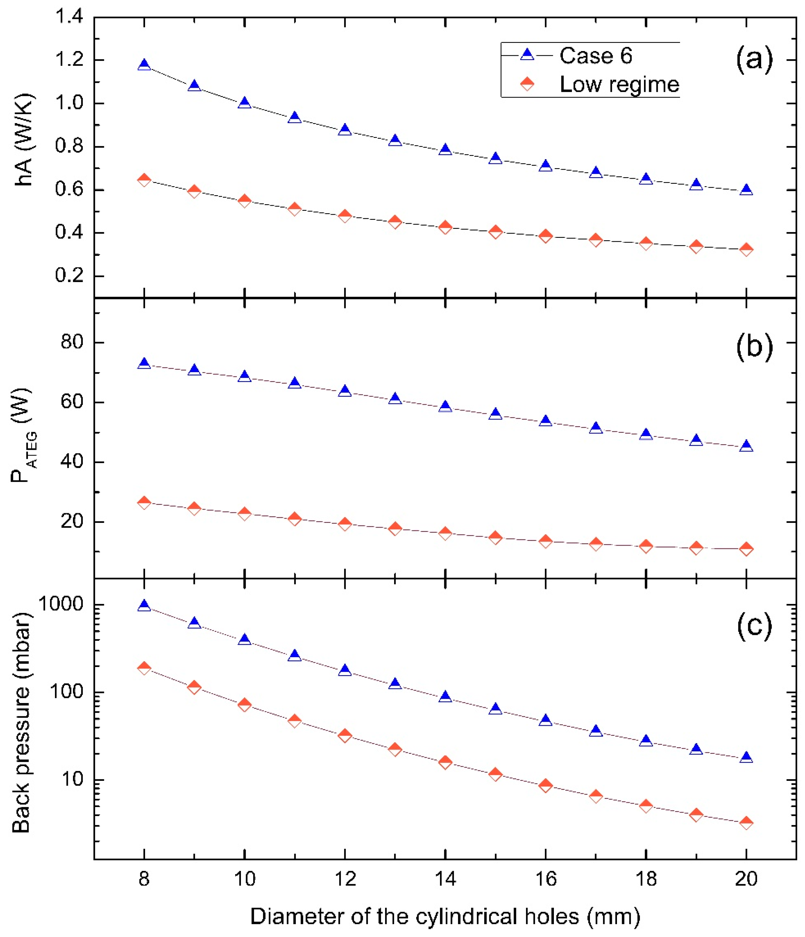
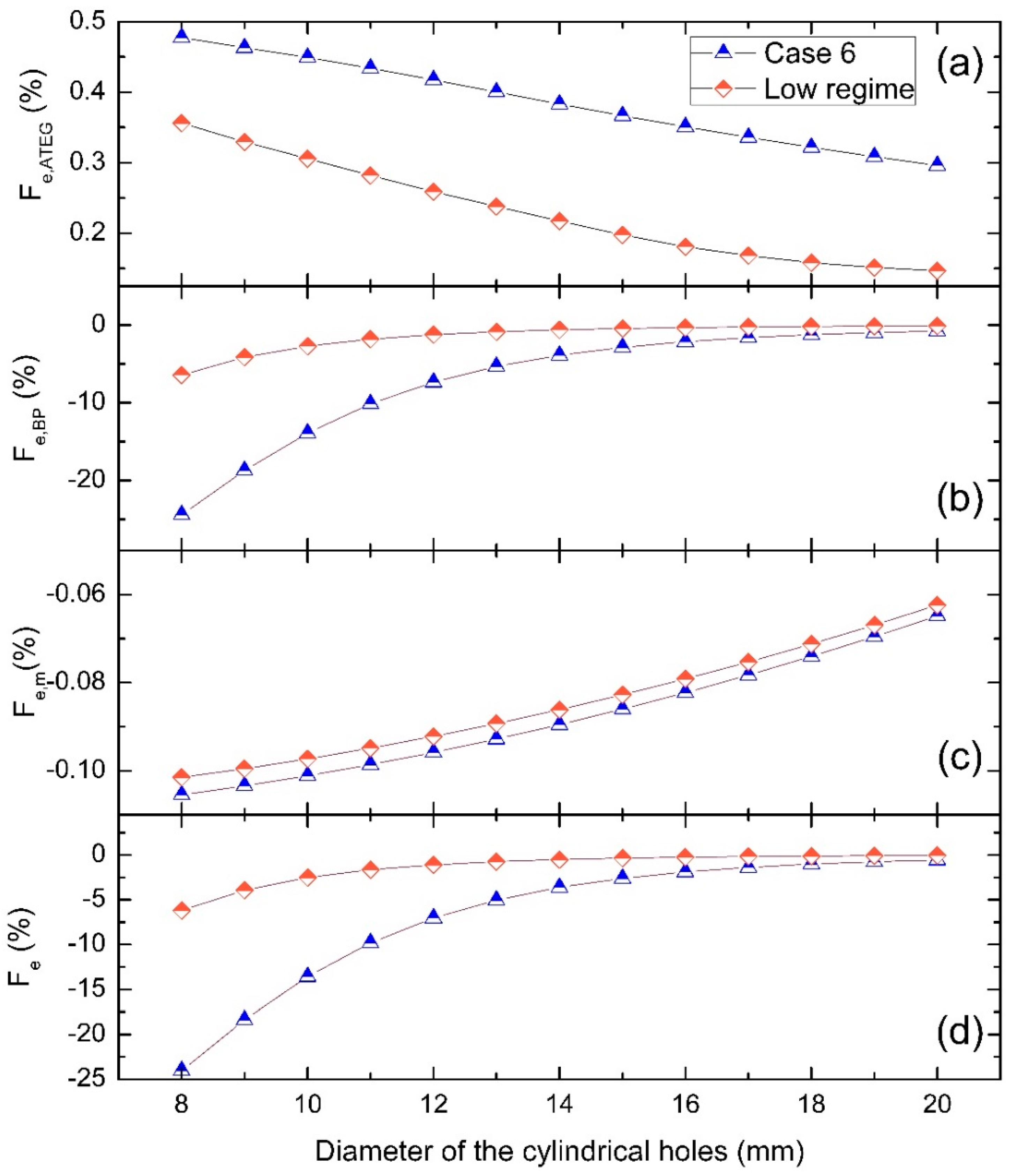
5.2. Heat Absorber: Effects of Changing the Diameter of the Cylindrical Holes

Previous results confirmed that back pressure is the main limiting factor to determining ATEG performance in terms of fuel consumption. Thus, actions intended to reduce the back pressure values should be focused on improving the design of the heat absorber. In our ATEG, the heat absorber was a copper block with six cylindrical holes of 12 mm inner diameter (Figure 1). As pointed out by other authors, this type of geometry generates more back pressure than heat absorbers based on fins, for example, Reference [7]. However, heat exchangers with cylindrical holes have some advantages over fin heat absorbers since the latter have constraints related to the type of material being used and the geometrical dimensions of the fin (minimum available fin spacing and fin thickness depending on the manufacturing techniques). The above implies that the cost of a fin-type heat absorber becomes higher than that with cylindrical holes. This is a very important issue when devices have to be mass produced. In addition, although not employed here, there are several passive methods to enhance heat transfer in heat absorbers with cylindrical holes such as, for example, inserting helical elements [45]. From the above, our goal was to investigate the potential heat absorbers with cylindrical holes had as heat transfer devices for the hot part of ATEGs, and how fuel consumption may be improved by changing a key design parameter: the diameter of the cylindrical hole.

The value of the convective heat transfer coefficient, h, multiplied by the exchange area, A, between the six inner cylindrical holes and the exhaust gas was calculated for different designs by varying the diameter D of the holes from 8 mm to 20 mm. Results with engine load operating conditions that gave the maximum P_ATEG value in the laboratory experiment (case 6 in Table 3) and with a low regime case (${\dot{m}}_g$ = 24.1 g/s, T_g,i = 454.8 °C, T_w,i = 20 °C, and ${\dot{V}}_w$ = 580 L/h, as in Reference [7]) are shown in Figure 15a. The trend of hA as a function of D followed the same behavior as in Figure 13b. Heat transfer was enhanced when the diameter of the holes was reduced because the increment in flow velocity increased the value of h which, in turn, clearly compensated for the small decrease in the exchange surface area A. Varying the convective thermal resistance modified the power output (as observed in Figure 15b). High values of hA led to high values of P_ATEG. Furthermore, the heat flow extracted from the exhaust gases can be approximated as $Q=hA\left(T_{ha}-T_g\right)$, where T_ha and T_g are the temperatures of the heat absorber and exhaust gases, respectively. Thus, the $P_{ATEG}/\left(hA\right)$ ratio can be understood as a measure of an energy conversion efficiency term of the ATEG multiplied by $\left(T_{ha}-T_g\right)$. For high values of D (>15 mm), $P_{ATEG}/\left(hA\right)$ for both regimes was almost constant, especially in the low regime case, thus indicating a constant conversion efficiency η. This coefficient was evaluated as η = P_ATEG/Q_h. For an engine operating point as in case 6, the maximum power attained with D = 8 mm was 73 W, whereas, with D = 20 mm, the ATEG produced 45 W. For the low regime case, $P_{ATEG}$ ranged from 26 W (D = 8 mm) to 11 W (D = 20 mm). The maximum ATEG conversion efficiency was achieved with D = 8 mm, reaching η = 1.68% under the same conditions as case 6 and only η = 1.1% in the low regime case. The minimum ATEG conversion efficiency corresponded to simulations using D = 20 mm, with values equal to η = 1.30% for case 6 and η = 0.65% for the low regime case.

However, the main effect that changing the diameter of the cylinders had was on the back pressure values (Figure 15c). The Δp_bp values changed by almost two orders of magnitude (Δp_bp = 955 mbar at D = 8 mm in comparison with Δp_bp = 17 mbar at D = 20 mm; case 6). The behavior of Δp_bp as a function of D almost perfectly fitted a power trend. Thus, the strategy of reducing the size of the diameters of the cylinders to increase heat transfer and, hence, electrical output power heavily penalized the back pressure. For example, a 14% increase in $P_{ATEG}$ implied an increase in Δp_bp = 449% (from D = 12 mm to D = 8 mm, case 6). Therefore, this action had dramatic consequences on the fuel economy values (Figure 16).

Individual contributions to the total fuel economy F_e (Equation (14)) are shown in Figure 16. The impact of $P_{ATEG}$ on fuel consumption (Equation (11); Figure 16a) as a function of D, followed the trend observed in Figure 15b for the electrical output power. However, the differences between both cases (high- and low-load engine regimes) were not as important as in Figure 15b because the engine-shaft power in the low regime case was only 12.4 kW (24.9 kW in case 6). The effect of the power generated by the ATEG led to maximum fuel savings of 0.48% (D = 8 mm, case 6) and 0.37% (D = 8 mm, low regime). The contribution to the fuel economy (in %) due to the electric power generated was in the order of one-quarter of the value of the thermodynamic efficiency of the ATEG device. However, the consequences of the increasing back pressure at the exhaust pipe caused a massive increase in fuel consumption F_e,BP (Figure 16b), almost two orders of magnitude more important than the fuel savings from F_e,ATEG (Figure 16a) with an ATEG design that used D = 8 mm.

Values of less than a 1% increase in fuel consumption due to F_e,BP were only obtained in designs that offered a back pressure level below 23 mbar (designs with D > 18 mm evaluated under case 6 conditions, and designs with D > 12 mm in the low regime case). With our design, values of back pressure as low as 5 mbar were attained with D = 18 mm in the low regime situation (F_e,BP = −0.19%).

On the other hand, the effect of the increase in vehicle mass due to the installation of the ATEG implied an increase in fuel consumption in the order of 22% of the F_e,ATEG value, varying slightly with D (Figure 16c). Values of F_e,m approached zero as D increased, because less material was required to build the ATEG’s heat absorber; thus, m_ATEG decreased. Despite its low contribution to the overall fuel economy provided by the ATEG (Figure 16d), this term may be a critical contribution when F_e,BP is in the order of F_e,ATEG. This was the case for the low regime condition at D = 20 mm, since F_e,ATEG = 0.15%, F_e,BP = −0.12%, and F_e,m = −0.06%, resulting in an overall fuel savings of F_e = −0.03%. However, under stationary conditions (as in the laboratory experiment) the contribution of F_e,m is neglected and the very same design would produce a positive fuel economy value (F_e = 0.03%).

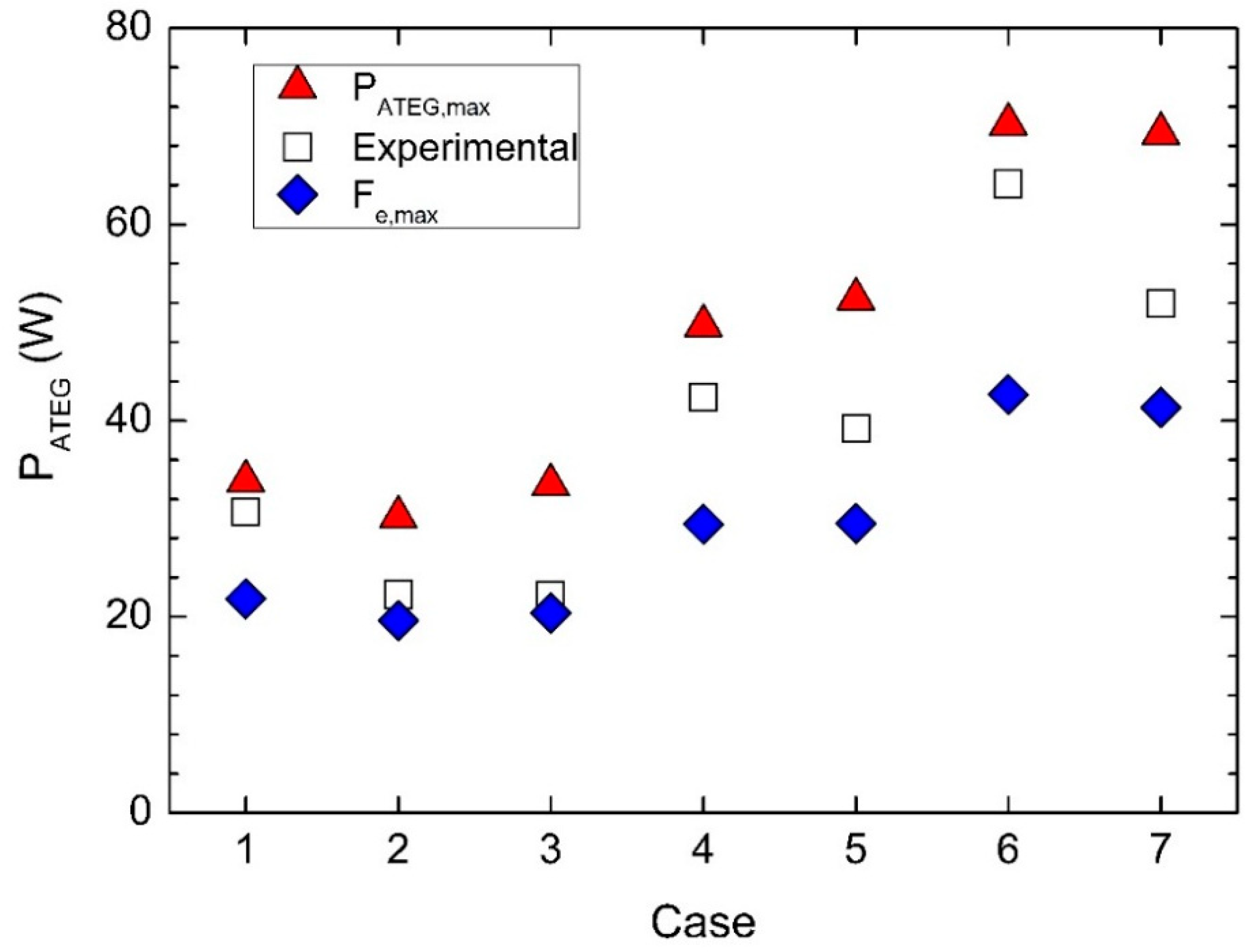
5.3. Configurations with Maximum Power and Maximum Fuel Economy

From the previous analyses, the back pressure emerged as the constraining factor for reaching fuel savings. However, the strategy to continuously reduce the back pressure may lead to designs that greatly reduce the amount of heat transferred to the ATEG, thus eventually obtaining very low electrical output power values. Although this may certainly imply positive numerical values of fuel economy, these savings are fictitious, since the amount of power injected into the system is so low that there is no sense in installing a whole ATEG device. This would be, for example, the case of the F_e = 0.03% case discussed above.

Thus, an ATEG feasibility study must implicitly accept two requisites: (1) electrical output power above a given threshold value (e.g., P_ATEG > 100 W), and (2) fuel savings above a given threshold value (e.g., F_e > 3%). Fulfilling the latter condition (fuel economy) would almost certainly imply achieving the first one (power). However, as we saw above, fulfilling the first condition (power) does not imply achieving minimum fuel savings.

Therefore, an interesting tool to assess the adequacy of the ATEG consisted of plots of output power and fuel savings corresponding to designs that maximized both terms (Figure 17 and Figure 18). Obviously, output power values obtained with design parameters that maximized fuel economy (D = 20 mm, ${\dot{V}}_w$ = 580 L/h, L = 8 mm) became smaller than those corresponding to the design that maximized output power (D = 8 mm, ${\dot{V}}_w$ = 580 L/h, L = 8 mm) (Figure 17). The experimental design approached either the condition of P_ATEG,max or of F_e,max depending on the cooling flow rate used in the test and, therefore, on the amount of heat flow transferred. Cases with low heat flow yielded low output power, similar to those attained with a heat absorber whose cylindrical holes were of a higher diameter (F_e,max case). All in all, the differences in P_ATEG between the designs at P_ATEG,max and at F_e,max were less than 44% with respect to the values of the P_ATEG,max design.

However, differences in fuel consumption values for both designs were much higher (Figure 18). Note that all values in Figure 18 provided negative values of F_e, meaning that not one combination of the design parameters studied led to fuel savings. In contrast with output power, fuel economy was much more sensitive to the main ATEG design parameters and, particularly, to the design of the heat absorber. The reason is that back pressure was the dominant term when calculating fuel economy values.

From Figure 18, we observed that the variability of the fuel consumption among the cases analyzed was not as high as among the output power values. For the P_ATEG,max design, for example, P_ATEG = 70 W for case 6 and P_ATEG = 30 W for case 2 (133% variation with respect to the latter case), whereas F_e = −24% for case 6 and F_e = −17% for case 1 (41% variation with respect to the latter case). A similar effect was observed for the F_e,max design. Thus, an initial estimation of the effect that back pressure values have on the fuel consumption does not require an evaluation of all the engine’s operational points.

In addition to the effects of the structural design, improvements in ATEG performance can also be obtained by adopting state-of-the-art electronic techniques to maximize power generation in transient behaviors (e.g., maximum power point tracking control [46]). Finally, the ongoing research into new thermoelectric materials is expected to substantially increase the actual values of figure of merit in commercial modules in future years [47,48]. Thus, it is interesting to provide a simple tool to determine the increment of the actual ZT_e value in order to have positive fuel savings. This was carried out by analyzing data of Figure 16. Each one of the three terms that contributed to the fuel economy could be expressed with equations of the form $F_{e,ATEG}(\%)=c_1{D}^2+c_{2}D+c_3$, $F_{e,BP}(\%)=c_4{e}^{c_{5}D}$, and $F_{e,m}(\%)=c_6{D}^2+c_{7}D+c_8$ with $c_1,\dots ,c_8$ constants. For case 6, the values of the coefficients were $c_1=0$ m⁻², $c_2=-0.0156$ m⁻¹, $c_3=0.603$, $c_4=-254.6$, $c_5=-0.2948$ m⁻¹, $c_6=1.21\times {10}^4$ m⁻², $c_7=-1.01\times {10}^6$ m⁻¹, and $c_8=-0.1132$, giving a square correlation coefficient greater than 0.998 in all of the three fits. $F_{e,ATEG}(\%)$ was directly proportional to P_ATEG when neglecting the contribution of the increase of pumping power of the cooling water (11), and, hence, to ZT_e by assuming no changes in the thermal and in the electrical conductivity of TEMs. Thus, the condition $r{F}_{e,ATEG}+F_{e,BP}+F_{e,m}=0$ would provide the ratio r of the new figure of merit to the actual one needed to reach a null variation in fuel consumption. For D = 20 mm in case 6, positive fuel savings would be achieved for r > 2.6 (i.e., TEMs 260% more efficient than the actual ones), implying an electrical output power equal to 118 W.

6. Conclusions

A numerical model of an ATEG based on the GT-SUITE software was developed. The model was validated with experimental data and correctly predicted the electrical output power and the back pressure. The model was used to study the consequences of modifying the cooling flow rate and the cross-sectional areas of (1) hot gases conduits in the heat absorber, and (2) water flow in the heat sink. Output power and fuel economy values were reported for different engine operating points. The main conclusions were as follows:

• Engine operating points of maximum output power did not coincide with those of maximum fuel economy.
• Designs that maximized output power differed substantially from those that maximized fuel savings.
• While an increase in the cooling flow rate enhanced the output power, it also increased the power required to pump the cooling flow. Therefore, a compromise between gaining generated power and the loss of power needed to drive the water pump must be made. From the design point, a maximum value of flow velocity in the cooling system should be imposed to assure that energy losses are not excessive. Changes in the cross-sectional area of the water cooling channel had a similar effect. From the initial layout, a reduction in flow rate was preferred over an increase in the cross-sectional area of the channel, since the former implied greater decrements of the required pumping power.
• The design of the heat absorber was critical in two opposing aspects: (1) to maximize the heat transfer, and (2) to minimize the back pressure. The back pressure was the main limiting factor in determining success in terms of fuel economy. Its value may vary several orders of magnitude depending on the type of heat absorber design. In order to have increments in fuel consumption <0.2% due to the effect of the back pressure, a value lower than 5 mbar should be attained.
• A heat absorber with cylindrical holes is not a recommended geometry since it leads to large back pressure values. For this type of heat absorber, the main three terms that contributed to fuel savings could be analytically expressed as a function of the diameter of the cylindrical holes with a high degree of accuracy. The analytical equations could be used to determine the minimum efficiency of the thermoelectric modules (figure of merit) in order to obtain positive fuel savings.
• The maximization of fuel savings cannot only rely on reducing back pressure values because this would result in trivial designs with very low back pressure and very low heat transfer being proposed. The feasibility of an ATEG requires a minimum value of electrical output power generated and this value should be kept as a constraint in the minimization study of the back pressure values.

Finally, it is worth noting that the present study had several limitations that can be resolved with future research. For example, the electrical connections were fixed in a series configuration since this was expected to provide the maximum output power. However, further investigation is required to determine whether or not hybrid (series/parallel) electrical configurations produce more electrical output power, especially in large ATEGs [35]. On the other hand, the fuel consumption calculations relied on analytical expressions that may deviate from observed data. Indeed, the goal of our ongoing research is to fully integrate the ATEG model into a complete simulation of a car within the GT-SUITE software and to validate its predictions with laboratory data. This full-vehicle model (including the ATEG) would provide very relevant information about the viability of this technology.

References

1. Rahman, A.; Razzak, F.; Afroz, R.; Akm, M.; Hawlader, M.N.A. Power generation from waste IC engines. Renew. Sustain. Energy Rev. 2015, 51, 382–395. [Google Scholar] [CrossRef]
2. Vázquez, J.; Palacios, R.; Sanz-Bobi, M.A. State of the art of thermoelectric generators based on heat recovered from the exhaust gases of automobiles. In Proceedings of the 7th European Workshop on Thermoelectrics, Pamplona, Spain, 3–4 October 2002. [Google Scholar]
3. European Commission. Clean Power for Transport: A European Alternative Fuels Strategy. Communication from the Commission to the European Parliament, the Council, the European Economic and Social Committee and the Committee of the Regions; COM (2013) 17; European Commission: Brussels, Belgium, 2013.
4. Karvonen, M.; Kapoor, R.; Uusitalo, A.; Ojanen, V. Technology competition in the internal combustion engine waste heat recovery: A patent landscape analysis. J. Clean. Prod. 2016, 112, 3735–3742. [Google Scholar] [CrossRef]
5. Massaguer, A.; Massaguer, E.; Comamala, M.; Pujol, T.; Montoro, L.; Cardenas, M.D.; Carbonell, D.; Bueno, A.J. Transient behavior under a normalized driving cycle of an automotive thermoelectric generator. Appl. Energy 2017, 206, 1282–1296. [Google Scholar] [CrossRef]
6. Fernández-Yáñez, P.; Armas, O.; Kiwan, R.; Stefaopoulou, A.G.; Boehman, A.L. A thermoelectric generator in exhaust systems of spark-ignition and compression-ignition engines. A comparison with an electric turbo-generator. Appl. Energy 2018, 229, 80–87. [Google Scholar] [CrossRef]
7. Comamala, M.; Pujol, T.; Cózar, I.R.; Massaguer, E.; Massaguer, A. Power and fuel economy of a radial automotive thermoelectric generator: Experimental and numerical studies. Energies 2018, 11, 2720. [Google Scholar] [CrossRef]
8. Stobart, R.; Wijewardane, M.A.; Yang, Z. Comprehensive analysis of thermoelectric generation systems for automotive applications. Appl. Therm. Eng. 2017, 112, 1433–1444. [Google Scholar] [CrossRef]
9. Matsubara, K. Development of a high efficient thermoelectric stack for a waste exhaust heat recovery of vehicles. In Proceedings of the 21st International Conference on Thermoelectronics, Proceedings ICT, Long Beach, CA, USA, 29 August 2002; pp. 418–423. [Google Scholar]
10. Kim, T.Y.; Kwak, J.; Kim, B.-W. Energy harvesting performance of hexagonal shaped thermoelectric generator for passenger vehicle applications: An experimental approach. Energy Convers. Manag. 2018, 160, 14–21. [Google Scholar] [CrossRef]
11. Orr, B.; Akbarzadeh, A.; Lappas, P. An exhaust heat recovery system utilizing thermoelectric generators and heat pipes. Appl. Therm. Eng. 2017, 126, 1185–1190. [Google Scholar] [CrossRef]
12. Haidar, J.G.; Ghojel, J.I. Waste heat recovery from the exhaust of low-power diesel engine using thermoelectric generators. In Proceedings of the 20th International Conference on Thermoelectrics, Proceedings ICT, Beijing, China, 8–11 June 2001; pp. 413–417. [Google Scholar]
13. Wang, Y.; Li, S.; Xie, X.; Deng, Y.; Liu, X.; Su, C. Performance evaluation of an automotive thermoelectric generator with inserted fins or dimpled-surface hot heat exchanger. Appl. Energy 2018, 218, 391–401. [Google Scholar] [CrossRef]
14. Thacher, E.F.; Helenbrook, B.T.; Karri, M.A.; Richter, C.J. Testing of an automobile exhaust thermoelectric generator in a light truck. Proc. Inst. Mech. Eng. Part D 2007, 221, 95–107. [Google Scholar] [CrossRef]
15. Lan, S.; Yang, Z.; Chen, R.; Stobart, R. A dynamic model for thermoelectric generator applied to vehicle waste heat recovery. Appl. Energy 2018, 210, 327–338. [Google Scholar] [CrossRef]
16. Frobenius, F.; Gaiser, G.; Rusche, U.; Weller, B. Thermoelectric generators for the integration into automotive exhaust systems for passenger cars and commercial vehicles. J. Electron. Mater. 2016, 45, 1433–1440. [Google Scholar] [CrossRef]
17. Bass, J.C.; Elsner, N.B.; Leavitt, F.A. Performance of the 1 kW thermoelectric generator for diesel engines. AIP Conf. Proc. 1994, 316, 295–298. [Google Scholar]
18. Massaguer, A.; Massaguer, E.; Comamala, M.; Pujol, T.; González, J.R.; Cardenas, M.D.; Carbonell, D.; Bueno, A.J. A method to assess the fuel economy of automotive thermoelectric generators. Appl. Energy 2018, 222, 42–58. [Google Scholar] [CrossRef]
19. Karri, M.A.; Thacher, E.F.; Helenbrook, B.T. Exhaust energy conversion of thermoelectric generator: Two case studies. Energy Convers. Manag. 2011, 52, 1596–1611. [Google Scholar] [CrossRef]
20. Champier, D. Thermoelectric generators: A review of applications. Energy Convers. Manag. 2017, 140, 167–181. [Google Scholar] [CrossRef]
21. Von Lukowicz, M.; Abbe, E.; Schmiel, T.; Tajmar, M. Thermoelectric generators on satellites-An approach for waste heat recovery in space. Energies 2016, 9, 541. [Google Scholar] [CrossRef]
22. Lv, H.; Li, G.; Zheng, Y.; Hu, J.; Li, J. Compact water-cooled thermoelectric generator (TEG) based on a portable gas stove. Energies 2018, 11, 2231. [Google Scholar] [CrossRef]
23. Li, G.; Zhang, G.; He, W.; Ji, J.; Lv, S.; Chen, X.; Chen, H. Performance analysis on a solar concentrating thermoelectric generator using the micro-channel heat pipe array. Energy Convers. Manag. 2016, 112, 191–198. [Google Scholar] [CrossRef] [Green Version]
24. Li, G.; Feng, W.; Jin, Y.; Chen, X.; Ji, J. Discussion on the solar concentrating thermoelectric generation using micro-channel heat pipe array. Heat Mass Transfer 2017, 53, 3249–3256. [Google Scholar] [CrossRef]
25. Li, G.; Chen, X.; Jin, Y. Analysis of the primary constraint conditions of an efficient photovoltaic-thermoelectric hybrid system. Energies 2017, 10, 20. [Google Scholar] [CrossRef]
26. Li, G.; Ji, J.; Zhang, G.; He, W.; Chen, X.; Chen, H. Performance analysis on a novel micro-channel heat pipe evacuated tube solar collector-incorporated thermoelectric generation. Int. J. Energy Res. 2016, 40, 2117–2127. [Google Scholar] [CrossRef]
27. Cheng, K.; Feng, Y.; Lv, C.; Zhang, S.; Qin, J.; Bao, W. Performance evaluation of waste heat recovery systems based on semiconductor thermoelectric generators for hypersonic vehicles. Energies 2017, 10, 570. [Google Scholar] [CrossRef]
28. Fernández-Yañez, P.; Armas, O.; Capetillo, A.; Martínez-Martínez, S. Thermal analysis of a thermoelectric generator for light-duty diesel engines. Appl. Energy 2018, 226, 690–702. [Google Scholar] [CrossRef]
29. He, W.; Zhang, G.; Li, G.; Ji, J. Analysis and discussion on the impact of non-uniform input heat flux on thermoelectric generator array. Energy Convers. Manag. 2015, 98, 268–274. [Google Scholar] [CrossRef]
30. Risseh, A.E.; Nee, H.-P.; Goupil, C. Electrical power conditioning system for thermoelectric waste heat recovery in commercial vehicles. IEEE Trans. Transp. Electrif. 2018, 4, 548–562. [Google Scholar] [CrossRef]
31. Demir, M.E.; Dincer, I. Performance assessment of a thermoelectric generator applied to exhaust waste heat recovery. Appl. Therm. Eng. 2017, 120, 694–707. [Google Scholar] [CrossRef]
32. He, W.; Wang, S.; Yue, L. High net power output analysis with changes in exhaust temperature in a thermoelectric generator system. Appl. Energy 2017, 196, 259–267. [Google Scholar] [CrossRef]
33. Kempf, N.; Zhang, Y. Design and optimization of automotive thermoelectric generators for maximum fuel efficiency improvement. Energy Convers. Manag. 2016, 121, 224–231. [Google Scholar] [CrossRef] [Green Version]
34. Gamma Technologies LLC. Available online: https://www.gtisoft.com (accessed on 1 October 2018).
35. Cózar, I.R.; Pujol, T.; Lehocky, M. Numerical analysis of the effects of electrical and thermal configurations of thermoelectric modules in large-scale thermoelectric generators. Appl. Energy 2018, 229, 264–280. [Google Scholar] [CrossRef]
36. National Instruments. Available online: http://www.ni.com (accessed on 3 September 2018).
37. Omega. Available online: http://www.omega.com (accessed on 3 September 2018).
38. Sensus. Available online: http://www.sensus.com (accessed on 3 September 2018).
39. Su, J.; Xu, M.; Li, T.; Gao, Y.; Wang, J. Combined effects of cooled EGR and a higher geometric compression ratio on thermal efficiency improvement of a downsized boosted spark-ignition direct engine. Energy Convers. Manag. 2014, 78, 65–73. [Google Scholar] [CrossRef]
40. Zhao, M.; Wei, M.; Song, P.; Liu, Z.; Tian, G. Performance evaluation of a diesel engine integrated with ORC system. Appl. Therm. Eng. 2017, 115, 221–228. [Google Scholar] [CrossRef] [Green Version]
41. Zhao, R.; Li, W.; Zhuge, W.; Zhang, Y.; Yin, Y. Numerical study on steam injection in a turbocompound diesel engine for waste heat recovery. Appl. Energy 2017, 185, 506–518. [Google Scholar] [CrossRef]
42. Incropera, F.P.; DeWitt, D.P.; Bergman, T.L.; Lavine, A.S. Fundamentals of Heat and Mass Transfer, 7th ed.; John Wiley & Sons, Inc.: Hoboken, NJ, USA, 2007. [Google Scholar]
43. Chen, J.; Li, K.; Liu, C.; Li, M.; Lv, Y.; Jia, L.; Jiang, S. Enhanced efficiency of thermoelectric generator by optimizing mechanical and electrical structures. Energies 2017, 10, 1329. [Google Scholar] [CrossRef]
44. Li, Z.; Li, W.; Chen, Z. Performance analysis of thermoelectric based automotive waste heat recovery system with nano fluid coolant. Energies 2017, 10, 1489. [Google Scholar] [CrossRef]
45. Alam, T.; Kim, M.-H. A comprehensive review on single phase heat transfer enhancement techniques in heat exchanger applications. Renew. Sustain. Energy Rev. 2018, 81, 813–839. [Google Scholar] [CrossRef]
46. Twaha, S.; Zhu, J.; Maraaba, L.; Huang, K.; Li, B.; Yan, Y. Maximum power point tracking control of a thermoelectric generation system using the extremum seeking control method. Energies 2017, 10, 2016. [Google Scholar] [CrossRef]
47. Xie, D.; Xu, J.; Liu, G.; Liu, Z.; Shao, H.; Tan, X.; Jiang, J.; Jiang, H. Synergistic optimization of thermoelectric performance in p-type Bi0.48Sb1.52Te3/graphene composite. Energies 2016, 9, 236. [Google Scholar] [CrossRef]
48. Zhao, D.; Wu, D.; Bo, L. Enhanced thermoelectric properties of Cu2SbSe4 compounds via gallium doping. Energies 2017, 10, 1524. [Google Scholar] [CrossRef]
Figure 1. (a) Main elements of the automative thermoelectric generator (ATEG; slightly modified from Reference [5]); (b) water channel path.
Energies 11 03274 g001
Figure 2. Schematic diagram of the laboratory set-up.
Energies 11 03274 g002
Figure 3. ATEG installed in the engine test bench.
Energies 11 03274 g003
Figure 4. (a) Schematic drawing of the test rig of thermoelectric modules (TEMs; dimensions in mm); (b) test rig of TEMs in the laboratory.
Energies 11 03274 g004
Figure 5. Block diagram of the ATEG model containing two cold-side heat exchangers (CSHEs), 12 TEMs, thermal connections (blue lines), flow connections (red lines), electrical connections (green lines), and the hot-side heat exchanger (HSHE).
Energies 11 03274 g005
Figure 6. Block diagram of thermal mass #1 of the HSHE including exhaust gas channels (red) and thermal connections (blue).
Energies 11 03274 g006
Figure 7. Block diagram of electrical and thermal connections of TEMs (1), indicating the thermal contact resistances (2), electrical node junctions (3), ground connection (4), and electrical load resistance (5).
Energies 11 03274 g007
Figure 8. Example of a thermal connection between the CSHE and the TEMs. (a) Dashed lines enclose the example zone; (b) block diagram with connections within the example zone.
Energies 11 03274 g008
Figure 9. Experimental and simulated results of (a) water cooling temperature at ATEG outlet (Tw,o), and (b) exhaust gas temperature at ATEG outlet (Tg,o), for those cases listed in Table 3.
Energies 11 03274 g009
Figure 10. Experimental and simulated results of (a) ATEG voltage, and (b) ATEG current.
Energies 11 03274 g010
Figure 11. Experimental and simulated results of the electrical output power of the ATEG (PATEG) for the cases listed in Table 3.
Energies 11 03274 g011
Figure 12. (a) Experimental and simulated results of back pressure obtained at the flow bench; (b) only the HSHE plus contraction and expansion cones of the ATEG were needed in the test.
Energies 11 03274 g012
Figure 13. (a) Contours of electrical output power (PTEG) normalized to the maximum value obtained (PTEG/PTEG,max; PTEG,max = 63.9 W); (b) contours of the product of the convective heat transfer multiplied by the area of the CSHE channel in contact with the water (hA) normalized to the maximum value obtained (hA/hAmax; hAmax = 9.54 W·K−1) as a function of the water coolant flow rate V ˙ w and height of the coolant channel L. All other conditions are as in case 6 in Table 3.
Energies 11 03274 g013
Figure 14. Contours of changes in fuel economy (Fe) relative to the maximum value (Fe/Fe,max −1; Fe,max = −7.01%) as a function of water coolant flow rate V ˙ w and height of coolant channel L. All other conditions as in case 6 of Table 3.
Energies 11 03274 g014
Figure 15. (a) Convective heat transfer coefficient multiplied by the contact area of gases with the heat absorber, (b) electrical output power, and (c) back pressure as a function of the diameter of the cylindrical holes for high (case 6 in Table 3) and low (see text) engine regime conditions.
Energies 11 03274 g015
Figure 16. (a) Fuel economy (%) due to the electrical power generated by the ATEG (Equation (11)), (b) fuel economy (%) due to the back pressure created by the ATEG (Equation (12)), (c) fuel economy (%) due to the increase in vehicle mass (Equation (13)), and (d) overall fuel economy (%) (Equation (14)) as a function of the diameter of the cylindrical holes for high (case 6 in Table 3) and low (see text) engine regime conditions.
Energies 11 03274 g016
Figure 17. Output power of the ATEG obtained with the design that maximizes output power (PATEG,max), the design that maximizes fuel economy (Fe,max), and the design tested in the laboratory (Experimental) for the operational conditions given in Table 3.
Energies 11 03274 g017
Figure 18. Fuel economy obtained with the design that maximizes output power (PATEG,max), the design that maximizes fuel economy (Fe,max), and the design tested in the laboratory (Experimental) for the operational conditions outlined in Table 3.
Energies 11 03274 g018