Modelling and Experimental Analysis of a Polymer Electrolyte Membrane Water Electrolysis Cell at Different Operating Temperatures

Abstract

In this paper, a simplified model of a Polymer Electrolyte Membrane (PEM) water electrolysis cell is presented and compared with experimental data at 60 °C and 80 °C. The model utilizes the same modelling approach used in previous work where the electrolyzer cell is divided in four subsections: cathode, anode, membrane and voltage. The model of the electrodes includes key electrochemical reactions and gas transport mechanism (i.e., H₂, O₂ and H₂O) whereas the model of the membrane includes physical mechanisms such as water diffusion, electro osmotic drag and hydraulic pressure. Voltage was modelled including main overpotentials (i.e., activation, ohmic, concentration). First and second law efficiencies were defined. Key empirical parameters depending on temperature were identified in the activation and ohmic overpotentials. The electrodes reference exchange current densities and change transfer coefficients were related to activation overpotentials whereas hydrogen ion diffusion to Ohmic overvoltages. These model parameters were empirically fitted so that polarization curve obtained by the model predicted well the voltage at different current found by the experimental results. Finally, from the efficiency calculation, it was shown that at low current densities the electrolyzer cell absorbs heat from the surroundings. The model is not able to describe the transients involved during the cell electrochemical reactions, however these processes are assumed relatively fast. For this reason, the model can be implemented in system dynamic modelling for hydrogen production and storage where components dynamic is generally slower compared to the cell electrochemical reactions dynamics.

1. Introduction

With the increasing production of electricity from intermittent renewable energy sources (e.g., wind and solar), the need for an effective energy storage is becoming imperative. It is therefore necessary to accumulate energy at the time it is not requested, and use it later when renewable energy is lacking, and energy is still demanded.

The European Union (EU-28) has seen an increased renewable energy production over the years and it is aiming to reach 20% of the gross final energy consumption by 2020. It is estimated that between 2006 and 2016 there was an increase in renewable energy production by two-thirds [1].

Among the different options for energy storage, PEM electrolysis has recently attracted attention because it utilizes the same technology as PEM fuel cells, which has been developed for a long time and proven successful. The electrolyzer is able to produce hydrogen from electricity by an electrochemical reaction for later use in a fuel cell, moreover hydrogen can be used to produce other carbon-neutral fuels such as syngas and alcohols (e.g., methanol) which despite containing carbon, can be produced by renewable sources [2,3].

Early electrolyzer models and simulations in Matlab/Simulink^® were developed among others by [4,5]. Such a dynamic modelling software platform is well suited for energy case scenarios where input and output are continuously changing over the time. In particular in [4], the authors describe a model with all the components from renewable energy generation including the wind turbines, electrolyzer, fuel cell and power conditioning. System transient responses to different case scenarios are also presented.

One of the first Simulink mathematical models of the gas porous diffusion electrode and ion exchange membranes of a PEM electrolyzer can be attributed to Görgün et al. [6]. This model is in fact a steady state model, as it does not consider thermal and electrical capacitance dynamic effects. Awasthi et al. [7] followed a similar approach.

Marangio et al. [8] presented a validated PEM electrolyzer semi-empirical model including overvoltages and resistances along the electrodes, flow plates and electrolyte. Abdin et al. [9] included Knudsen diffusion and molecular diffusion to characterize cathode and anode porous media. Choi et al. [10] developed an electrolyzer model with the Butler-Volmer kinetics including the effect of cell temperature on the exchange current density. More recently, Yigit et al. [11] developed a dynamic model of a high pressure PEM electrolyzer system, the model is only partially validated. This study gives detailed information of the energy losses in the system at different current density of the electrolyzer showing that above 1 A/cm² efficiency become significantly low.

In the aforementioned models, authors implemented the differential equations describing the physical phenomena directly in the software platform. Other authors have found other ways to approach this complex dynamic system modelling effort. For instance, Olivier et al. [12] developed a model based on the “bond graph” method. The model includes stack and BoP and simulates the behavior under intermittent condition. This graphical approach is helpful to simplify the representation of complex dynamic system behavior and convert the system in a state-space mode. The model was then implemented in Matlab/Simulink^®, showing good agreement between experimental and model data.

Zhou et al. [13] developed a control oriented electrolyzer model and tested it in real time with a hardware-in-the-loop emulator of the electrolyzer and wind energy system. The emulator is able to test different electrolyzer specifications given by the manufacturers. In [14], Ruuskanen et al. followed a similar approach where only the power conditioning was experimentally tested and the rest of the system was implemented in a power-hardware-in-loop.

This paper provide a validated PEM electrolyzer model that includes the physical principles introduced in previous papers [4,5,8,9]. In addition, in this study we estimate cell efficiency and heat dissipation. Besides differently from [8,9], water gas pressure was calculated using the water saturation pressure. The model is able to predict cell performance at a large range of different temperatures. Exchange current densities parameters and membrane conductivity was chosen as closely depending on temperature.

This study is divided in two main parts. In the first part, the experimental test is described where an electrolyzer cell is characterized and performance are measured. In the second part, the model is detailed described and the experimental results are used to validate the model.

2. Experimental

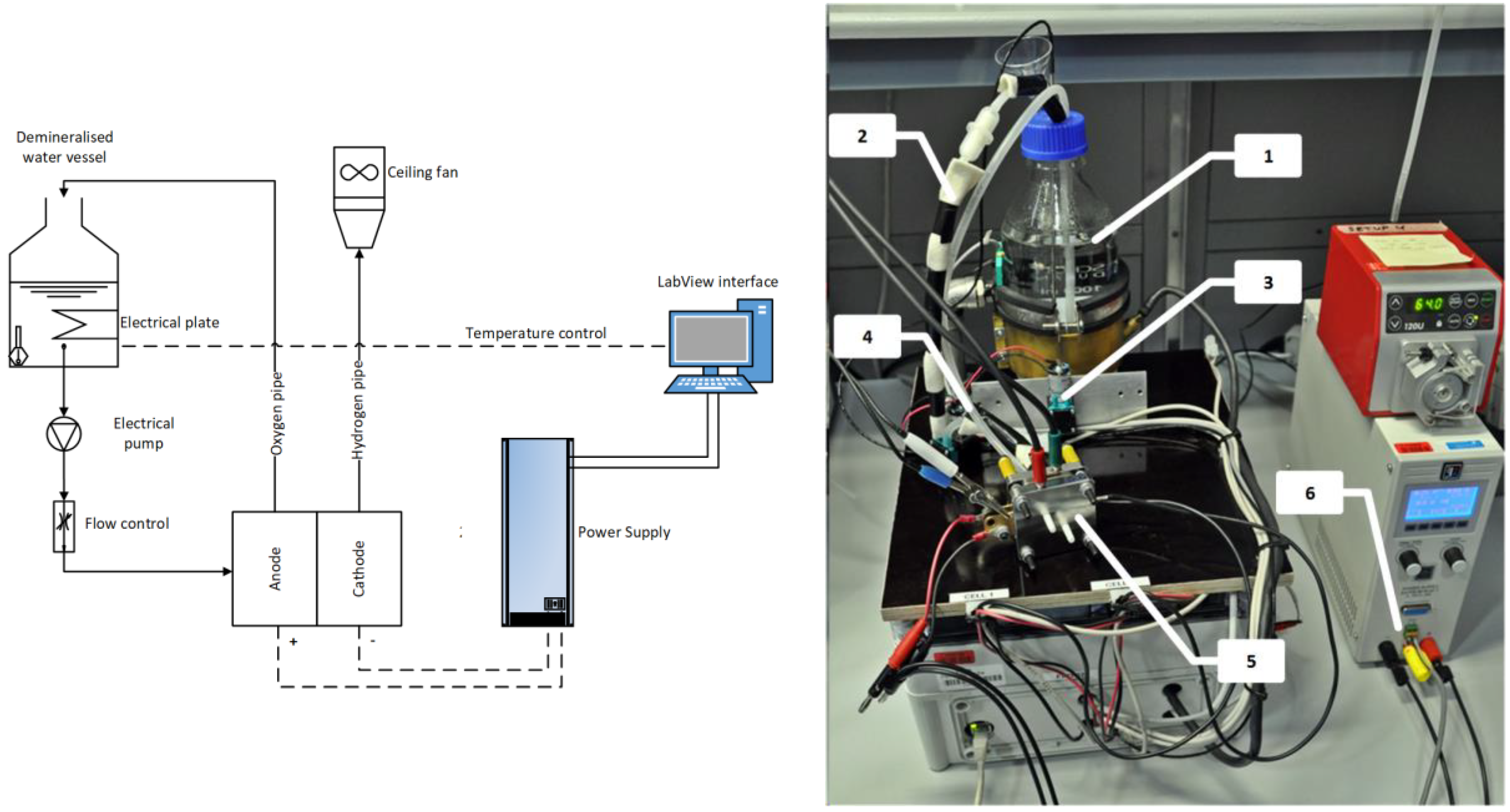
The experimental setup is shown in Figure 1. The core of test is the electrolyzer cell assembly that is supplied by electrical power and the required reactants. The polarization curve was registered at two fixed operating temperatures, i.e., 60 °C and 80 °C. A start-up phase initiated each test in which the cell gradually reached the set temperature.

The cell has an active area of 2.89 cm². The cathode has a catalyst loading of 0.5 mg/cm² Pt/C, carbon cloth (C-cloth PTL) with parallel flow field. The anode has a catalyst loading of 0.3 mg/cm² IrO2, 2.7 mg/cm² Ir, porous Ti PTL, with an interdigitated flow field. The Nafion polymer membrane is type N117.

Since the first part of the cell polarization curve has a greater slope, measurement were more frequent at lower current densities than at high current density. At each step, the voltage was measured as average of 3 min measurements. Up to 0.289 A, steps were every 0.01 A cm²; between 0.289 A and 0.578 A, steps were every 0.1 A cm². Finally, steps were every 0.2 A cm², from 0.578 A up to the maximum voltage which was fixed at 2.2 A.

3. Modelling

A simplified mathematical model was developed in Matlab/Simulink^®. The approach follows the same modelling structure initiated by Abdin et al. [9] and Marangio et al. [8]. The model is divided into four sub-sections: Anode and Cathode chambers, Membrane and Voltage.

The model was fitted to experimental electrolyzer polarization curve operating at 60 °C and 80 °C. The electrodes reference exchange current densities at the anode and cathode, electrodes charge transfer coefficients and the membrane hydrogen ion diffusivity were estimated from the cell curve performance as they closely relate to the cell performance at different temperature.

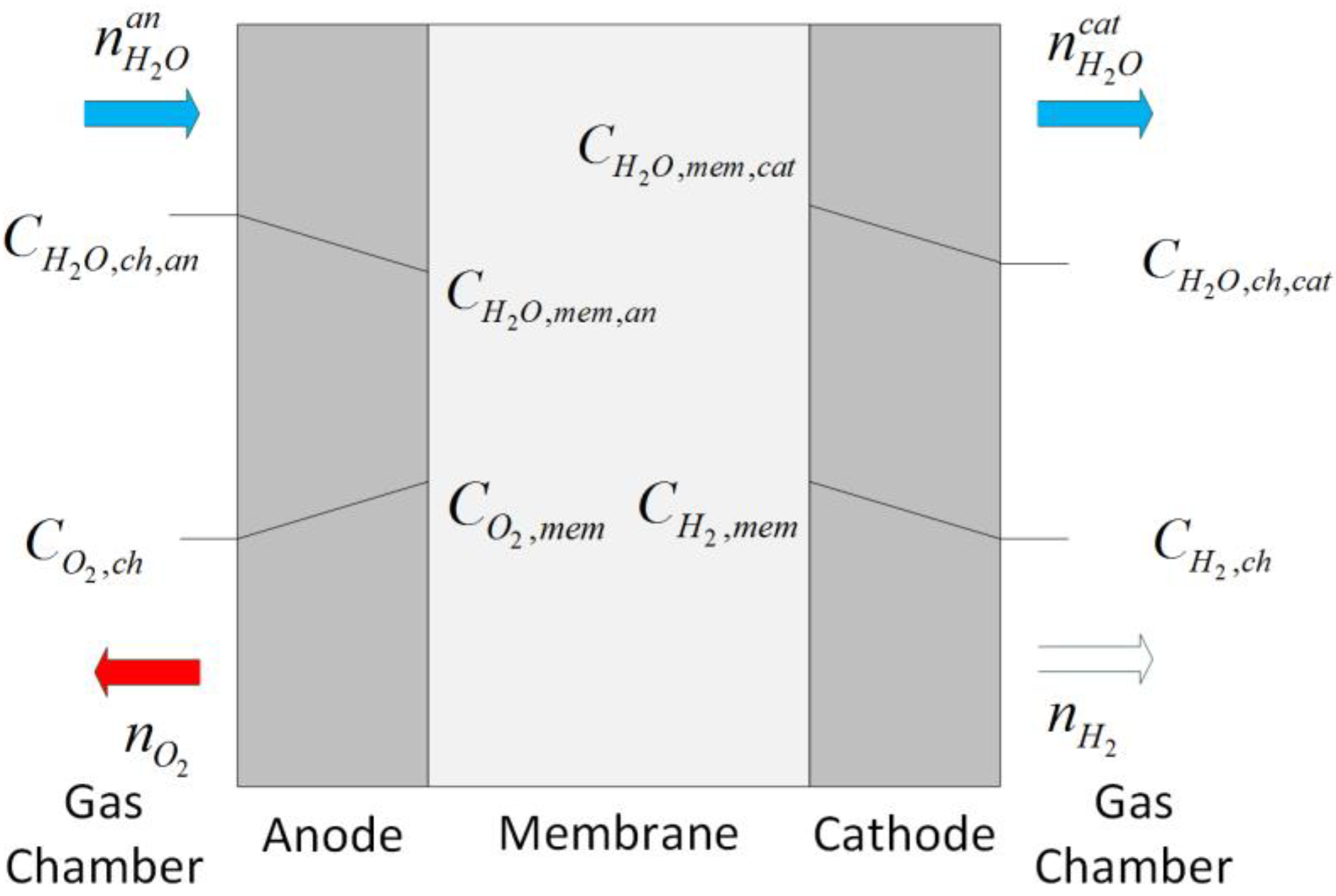
As Figure 2 depicts at the anode side, water is introduced and then split into hydrogen ions and oxygen gas. Hydrogen positive ions cross the membrane and recombine at the cathode side forming hydrogen gas. At the same time electrons travel through the external circuit, which is connected to the power supply that provide the electromotive force for the electrochemical reaction to happen. The basic reactions taking place to the electrolyte/electrode interface are given below:

$$\mathrm{Anode}: H_{2}O\to 2H^{+}+\frac{1}{2}{O}_2+2e^{2-}$$

(1)

$$\mathrm{Cathode}: 2H^{+}+2e^{-}\to H_2$$

(2)

$$\mathrm{Net} \mathrm{reaction}: H_{2}O\to H_2+\frac{1}{2}{O}_2$$

(3)

The model follows similar approach to the one used by Görgün in [6] and later by [6,9]. The model is divided in four Simulink blocks in which mass flow rate of different species are computed (i.e., Anode chamber, Cathode chamber, Membrane, Voltage). Main assumption of this model is to consider steady-state electrochemical mechanism for the electrolyzer model and therefore there is an instantaneous response to input changes with no time delays. This approach is justified by the fact that transient response is very fast in PEM electrolyzer as shown in experimental work by [6,9].

3.1. Anode Chamber

In the anode chamber, four moles of oxygen are generated for each electron. According to the “Faraday’s law” we can define the molar flow rate of generated oxygen as:

$${\dot{N}}_{an,O_2}^{gen}=\frac{I}{4F} \left[\mathrm{mol}/\mathrm{s}\right]$$

(4)

Similarly, two moles of water are consumed for each electron.

$${\dot{N}}_{an,H_{2}O}^{cons}=\frac{I}{2F} \left[\mathrm{mol}/\mathrm{s}\right]$$

(5)

$I$ is the current which is function of the current density, $i$, and the cell area, $A$, i.e., $I=iA$.

The accumulation of oxygen gas in the anode chamber is calculated as the difference between the oxygen gas at the chamber inlet and outlet plus the oxygen generated by the electrochemical reaction [9]:

$$\frac{d{N}_{an,O_2}}{dt}={\dot{N}}_{an,O_2}^{in}-{\dot{N}}_{an,O_2}^{out}+{\dot{N}}_{an,O_2}^{gen} \left[\mathrm{mol}/\mathrm{s}\right]$$

(6)

Similarly the accumulation of water takes into account the water consumed by the electrochemical reaction and the net water flow through the membrane which is the combination of multiple processes as described in section “Membrane” [9].

$$\frac{d{N}_{an,H_{2}O}}{dt}={\dot{N}}_{an,H_{2}O}^{in}-{\dot{N}}_{an,H_{2}O,l}^{out}-{\dot{N}}_{an,H_{2}O}^{cons}-{\dot{N}}_{H_{2}O}^{mem} \left[\mathrm{mol}/\mathrm{s}\right]$$

(7)

The partial pressure of the species in the channel can be calculated using the “Dalton law” in which oxygen, water and hydrogen are considered in the gas phase. Such an approach was used, among others, in [8,9]. As in the anode chamber water is in liquid phase, we calculate the oxygen gas partial as a difference between the anode total pressure and the water saturation pressure. In this way, the water gas phase is accounted equal to its saturation pressure.

In the present study, the anode pressure was considered atmospheric, i.e., $p_{an}=\mathrm{101,325} \mathrm{Pa}$

$$p_{O_2}=p_{an}-p_{H_{2}O,sat} \left[\mathrm{Pa}\right]$$

(8)

The water saturation pressure can be calculated using the “Antoine equation” which is function of temperature and other parameters shown in

Table 1. Parameter for the Antoine equation with T [°C] and p_sat [mm Hg] [15].

A	B	C	Tmin	Tmax
807.131	1730.63	233.426	1	100

:

$$p_{H_{2}O,sat}={10}^{A-\frac{B}{C+T}} \left[\mathrm{Pa}\right]$$

(9)

Similar approach for the gas species partial pressures calculation was used for the cathode.

3.2. Cathode Chamber

At the cathode side, hydrogen is generated by the electrochemical reaction. The molar balance and the gas partial pressure can be calculated similarly to the anode side.

The hydrogen gas accumulation is calculated as a difference between the hydrogen molar flow rate at the inlet and outlet plus the product hydrogen:

$$\frac{d{N}_{H_2}}{dt}={\dot{N}}_{H_2}^{in}-{\dot{N}}_{H_2}^{out}+{\dot{N}}_{H_2}^{gen} \left[\mathrm{mol}/\mathrm{s}\right]$$

(10)

$$\frac{d{N}_{H_{2}O}}{dt}={\dot{N}}_{H_{2}O}^{in}-{\dot{N}}_{H_{2}O}^{out}+{\dot{N}}_{H_{2}O}^{mem} \left[\mathrm{mol}/\mathrm{s}\right]$$

(11)

Product hydrogen is calculated using “Faraday’s law” considering that for two moles of electrons one mole of hydrogen is generated:

$${\dot{N}}_{H_2}^{gen}=\frac{I}{2F} \left[\mathrm{mol}/\mathrm{s}\right]$$

(12)

The hydrogen partial pressure is calculated as a difference between the cathode pressure, $p_{cat}=\mathrm{101,325} \mathrm{Pa}$, and the water saturation pressure:

$$p_{H_2}=p_{cat}-p_{H_{2}O,sat} \left[\mathrm{Pa}\right]$$

(13)

3.3. Membrane

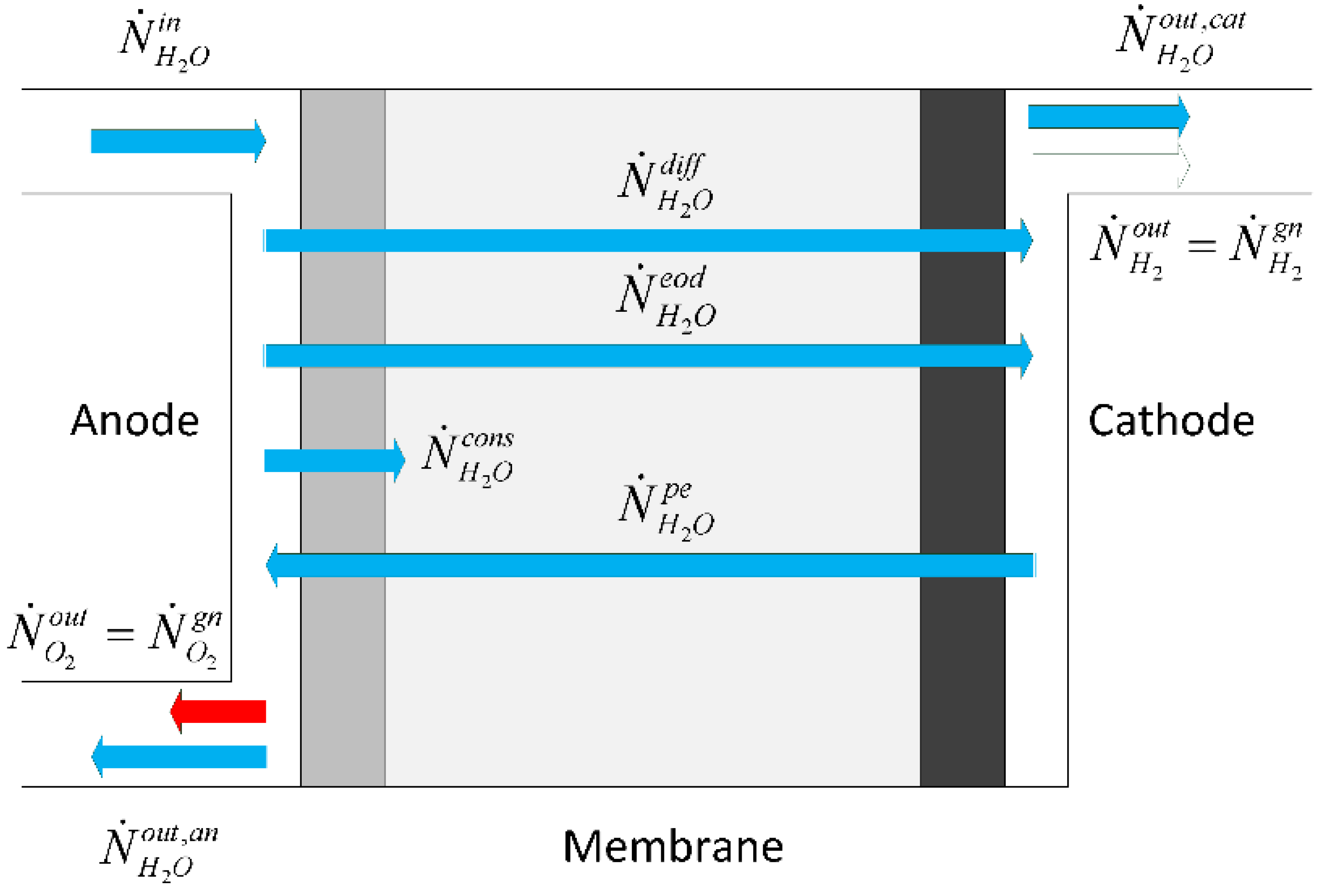
Abdin et al. [9] identify three main relevant phenomena for water transport, namely diffusion, electro osmotic drag and hydraulic pressure, which combined provide the membrane net water flow:

$${\dot{N}}_{H_{2}O}^{mem}={\dot{N}}_{H_{2}O}^{diff}+{\dot{N}}_{H_{2}O}^{eod}-{\dot{N}}_{H_{2}O}^{pe} \left[\mathrm{mol}/\mathrm{s}\right]$$

(14)

Diffusion mechanism refers to the transport phenomena due to concentration gradients across the membrane, whereas electro-osmotic drag refers to water which is dragged by hydrogen protons in the membrane, and hydraulic pressure refers to pressure asymmetries between the anode and cathode that cause water transport. We describe these three water transport processes in the next three sections.

3.4. Water Diffusion

Diffusion of water refers to the transport of water from high to low concentration regions prevalently from anode to cathode as water is formed at anode side. Fick’s law is used to calculate the water transport by integrating water concentration across the membrane between the two electrodes [16]:

$${\dot{N}}_{H_{2}O}^{diff}=A{D}_w\frac{d{c}_w}{dy}=\frac{A}{{\delta }_{mem}}{\displaystyle \underset{{{\displaystyle c}}_w^{anode}}{\overset{{{\displaystyle c}}_w^{cathode}}{\int }}{D}_{w}dy} [\mathrm{mol}/\mathrm{s}]$$

(15)

Water diffusion is function of active area of the membrane $A$, the water diffusion coefficient, $D_w$, and the water concentration in the membrane, $c_w$. In Figure 3, the concentration of the species at the membrane interface and inside the membrane is illustrated. We can assume that the water concentration at the electrode/membrane interface is approximated with the water concentration in the electrode channel.

Assuming a linear water concentration gradient, we can simply calculate the concentration gradients across the membrane as a difference instead of using integral function [8,9,11,17]. With this assumption in mind, we calculate the water molar flow rate due to diffusion as:

$${\dot{N}}_{H_{2}O}^{diff}=\frac{A{D}_w}{{\delta }_{mem}}(C_{H_{2}O}{}_{,mem,cat}-C_{H_{2}O}{}_{,mem,an}) [\mathrm{mol}/\mathrm{s}]$$

(16)

where $D_w$ is the membrane water diffusion coefficient, ${\delta }_{mem}$ is the thickness of the membrane and $C_{H_{2}O}{}_{,mem,cat}$, $C_{H_{2}O}{}_{,mem,an}$ are the water concentration at the electrolyte/electrode interfaces.

The diffusion process of a multi-component gas mixture across the electrode porous media is accounted using the Stefan-Maxwell approach, which considers an effective binary diffusion coefficient. Such a coefficient is used to estimate the diffusivity as a function of temperature, pressure and other geometric parameters [18]. Similarly to the approach described in [3,8], we can calculate the water concentration using the Fick’s law of diffusion in the electrolyte as shown in the equations below:

$$C_{H_{2}O}{}_{,mem,cat}=C_{H_{2}O}{}_{,ch,cat}+\frac{{\delta }_{el}^{cat}{n}_{H_{2}O}^{cat}}{D_{eff,cat}^{H_2-H_{2}O}} \left[\mathrm{mol}/\mathrm{L}\right]$$

(17)

$$C_{H_{2}O}{}_{,mem,an}=C_{H_{2}O}{}_{,ch,an}-\frac{{\delta }_{el}^{an}{n}_{H_{2}O}^{an}}{D_{eff,an}^{O_2-H_{2}O}} \left[\mathrm{mol}/\mathrm{L}\right]$$

(18)

where $D_{eff,an}^{O_2-H_{2}O}$ is the anode effective binary diffusion coefficient for $O_2-H_{2}O$, $D_{eff,cat}^{H_2-H_{2}O}$ is the cathode effective binary diffusion coefficient for the gas pair $H_2-H_{2}O$, ${\delta }_{el}^{an}$ and ${\delta }_{el}^{cat}$ are the thicknesses of the electrodes and $C_{H_{2}O}{}_{,ch,an}$ and $C_{H_{2}O}{}_{,ch,cat}$ are the water gas molar concentration.

The anode and cathode electrodes effective binary diffusion coefficient of transport, $D_{eff}$, is calibrated by applying the porosity correction [7,8]:

$$D_{eff,A-B}=D_{A-B}\epsilon {\left(\frac{\epsilon -{\epsilon }_p}{1-\epsilon }\right)}^{\alpha } \left[{\mathrm{cm}}^2/\mathrm{s}\right]$$

(19)

$\epsilon$ is the porosity correction, ${\epsilon }_p$ is the percolation threshold and $\alpha$ is an experimental factor. The binary diffusion coefficient is a proportionality factor that depends on temperature and pressure of generic two gas species A and B:

$$D_{A-B}=\left(a{\left(\frac{T}{\sqrt{T_{c,a}{T}_{c,b}}}\right)}^b{\left(p_{c,a}{p}_{c,b}\right)}^{\frac{1}{3}}{\left(T_{c,a}{T}_{c,b}\right)}^{\frac{5}{12}}{\left(\frac{1}{M_{m,A}}+\frac{1}{M_{m,B}}\right)}^{\frac{1}{2}}\right)\frac{1}{p} \left[{\mathrm{cm}}^2/\mathrm{s}\right]$$

(20)

In the equation, $p$ is the electrode pressure, $a$ and $b$ are coefficients that depends on the gas type, $M_m$ is the molar mass of species A and B. The water concentration in liquid form at anode and cathode can be expressed as:

$$C_{H_{2}O}{}_{,ch,cat}=\frac{{\rho }_{H2O}(T_{cat})}{M_{m,H2O}}; C_{H_{2}O}{}_{,ch,an}=\frac{{\rho }_{H2O}(T_{an})}{M_{m,H2O}} \left[\mathrm{mol}/\mathrm{L}\right]$$

(21)

The water density in this equation is calculated as [19]:

$$\rho =A/B^{1+{\left(1-\frac{T}{C}\right)}^D} \left[\mathrm{Kg}/{\mathrm{m}}^3\right]$$

(22)

The empirical parameters, A, B, C and D are provided in

Table 2. Parameter for the water density equation with T [K] [19].

A	B	C	D	${\mathit{T}}_{\min } \left[\mathbf{K}\right]$	${\mathit{T}}_{\max } \left[\mathbf{K}\right]$
0.14395	0.0112	649.727	0.05107	273	685

.

3.5. Electro Osmotic Drag

The water transport due to electro osmotic drag ${\dot{N}}_{H_{2}O}^{eod}$ represents the number of moles of water molecules which are dragged by each mole of hydrogen ions through the membrane and it is proportional to the osmotic drag coefficient and the hydrogen ions i.e., $I/F$.

$${\dot{N}}_{H_{2}O}^{eod}=\frac{n_{d}I}{F} \left[\mathrm{mol}/\mathrm{L}\right]$$

(23)

The osmotic drag coefficient, $n_d$, represents the number of water molecules carried by each hydrogen ions and it has been measured experimentally by different authors and resulted values have shown large variance. Awasthi et al. considered a value $n_d=5$ which is in line with the relationship below that is function of temperature and pressure [17]:

$$n_d=0.0252P_c-1.9073i+0.0189T_m-2.7892 \left[{\mathrm{mol}}_{\mathrm{H}2\mathrm{O}}/{\mathrm{mol}}_{\mathrm{H}+}\right]$$

(24)

In this work we consider the experimental relationship by Onda et al. [20] which applies to a fully hydrated membrane:

$$n_d=0.0134T+0.03 \left[{\mathrm{mol}}_{\mathrm{H}2\mathrm{O}}/{\mathrm{mol}}_{\mathrm{H}+}\right]$$

(25)

3.6. Hydraulic Pressure

Water transport due to pressure asymmetry, $\Delta p$, between anode and cathode depends on permeability of the membrane and can be calculated using the Darcy’s Law. Similar approach was followed by [7,8,9,17]. The relationship is function of the membrane permeability to water, $K_{darcy}$, the viscosity, ${\mu }_{H_{2}O}$, and the molar mass of water, $M_{m,H_{2}O}$:

$${\dot{N}}_{H_{2}O}^{pe}=K_{darcy}\frac{A{\rho }_{H_{2}O}}{{\delta }_{mem}{\mu }_{H_{2}O}{M}_{m,H_{2}O}}\Delta p \left[\mathrm{mol}/\mathrm{s}\right]$$

(26)

4. Voltage

The electrolyzer voltage is the sum of the cell potential at open circuit, $V_{oc}$, and three overpotentials $V_{act}$, $V_{ohm}$ and $V_{con}$:

$$V=V_{oc}+V_{act}+V_{ohm}+V_{con} \left[\mathrm{V}\right]$$

(27)

Below we provide the description of the four voltage components included in this model. The three overpotentials are called non faradaic losses as they are mainly caused by mass transport and resistance to the flow of protons in the electrolyte membrane and electric current in the cell components as described in Chapter 2 of [21].

4.1. Open-Circuit Voltage (OCV), $V_{oc}$

Equilibrium electrical potential is usually described by the Nernst equation [9]:

$$V_{oc}=V_{rev}^0-\frac{RT}{zF}\ln \left(\frac{a_{H_{2}O}}{a_{H_2}\cdot a_{O_2}^{1/2}}\right) \left[\mathrm{V}\right]$$

(28)

The reversible cell voltage, $V_{rev}^0$, and the species activities, a, can be rewritten using the partial pressure instead:

$$V_{oc}=E^0+\frac{RT}{zF}\ln \left(\frac{p_{H_2}}{p_{cat}}\sqrt{\frac{p_{O_2}}{p_{an}}}\right) \left[\mathrm{V}\right]$$

(29)

The reversible cell voltage is E⁰ is expressed as:

$$E^0=\frac{\Delta G_R^0}{zF} \left[\mathrm{V}\right]$$

(30)

4.2. Activation over Potential, $V_{act}$

The activation overvoltage can be deduced by the Butler-Volmer equation, which accounts for the electrochemical kinetics of the reaction. $V_{act}$ can be made explicit as follows:

$$V_{act}=\frac{RT}{\alpha F}\arcsin h\left(\frac{i}{2i_0}\right) \left[\mathrm{V}\right]$$

(31)

where, $\alpha$, is the charge coefficient. The activation overpotential represents the potential difference above the equilibrium potential (i.e., OCV) required to overcome the activation barriers to transfer electrons from the electrolyte to the electrode. The same relationship can be applied to anode and cathode electrodes of the electrolyzer cell so that the final value will be the sum of anode and cathode overpotentials:

$$V_{act}=V_{act}^{an}+V_{act}^{cat} \left[\mathrm{V}\right]$$

(32)

$i_0$ represents the exchange current density value which is function of the physical characteristics of the membrane material and catalyst and temperature of operation [8,9,22]. $i_0$ is computed both for anode and cathode and can be represented using the same expression used by [8,18] in which $i_0$ is function of the roughness factor ${\gamma }_M$ and the exchange current density, $i_0^{*}$ depending on temperature:

$$i_0={\gamma }_M{i}_0^{*} \left[\mathrm{A}/{\mathrm{cm}}^2\right]$$

(33)

The roughness factor ${\gamma }_M$ [23] is the ratio between the electrochemically active area and the geometric area of the membrane electrolyte assembly [23]:

$${\gamma }_M={\phi }_I{m}_M\frac{6}{{\rho }_M{d}_M} \left[{\mathrm{cm}}^2/{\mathrm{cm}}^2\right]$$

(34)

In the equation, ${\rho }_M$ is the catalyst density, $m_M$ is the catalyst leading, $d_M$ is the supported or unsupported catalyst crystallite diameter, ${\phi }_I$ is the fraction of metal catalyst surface in contact with the ionomer.

The exchange current density temperature dependence is modelled though an Arrhenius type relationship according to similar models [23,24,25]:

$$i_0^{*}=i_{0,ref}{e}^{\left[-\frac{E_a}{R}\left(\frac{1}{T}-\frac{1}{T_{ref}}\right)\right]} \left[\mathrm{A}/{\mathrm{cm}}^2\right]$$

(35)

where $i_{0,ref}$ is the exchange current density at reference temperate, $T_{ref}$. $i_{0,ref}$ for both anode and cathode was empirically fitted to the experimental data at reference temperature, $T_{ref}$.

4.3. Ohmic Overpotential, $V_{ohm}$

The ohmic overpotential is dominated by ionic loss predominantly in the membrane [8,9,11,23,25]:

$$V_{ohm}^{mem}=\frac{{\delta }_{mem}}{{\sigma }_{mem}}i \left[\mathrm{V}\right]$$

(36)

The ohmic voltage is dependent on the membrane thickness, ${\delta }_{mem}$, and the membrane conductivity, ${\sigma }_{mem}$. In many studies (e.g., the membrane conductivity, ${\sigma }_{mem}$, is expressed as a function of the membrane water content, $\lambda$, defined as the moles of water molecules for each mole of Sulfonic acid group, SO³⁻, in the Nafion membrane. $\lambda$ is generally constant in the electrolyzer case as the membrane is fully hydrated. In this study, ${\sigma }_{mem}$, was estimated using the relationship suggested by Bernardi and Verbrugge [18]:

$${\sigma }_{mem}=\frac{F^2{C}_{H^{+}}{D}_{H^{+}}}{RT} \left[\mathrm{S}/\mathrm{cm}\right]$$

(37)

The relationship depends on $C_{H^{+}}$ and $D_{H^{+}}$, which are the membrane concentration and diffusivity of hydrogen ions, $H^{+}$, the only two mobile ions, and they strongly influence performance. For our case, we considered a fixed value of $C_{H^{+}}=1000 \mathrm{mol}/{\mathrm{m}}^3$ as suggested in [6]. The temperature dependent $D_{H^{+}}$ value was empirically estimated to match experimental polarization curve.

4.4. Concentration over Potential, $V_{con}$

Marangio et al. [6] refer to this class of overpotential as “diffusion” overpotential as it considers the potential difference due to concentration difference of charge-carriers between the electrolyte and electrode surface. This mass flow in the membrane is unually described using the Nerst potential and calculating the voltage loss from a reference concentration [26].

The derivation and expression below is from [6]:

$$V_{con}=V_1-V_0=\frac{RT}{zF}\ln \frac{C_1}{C_0} \left[\mathrm{V}\right]$$

(38)

where $C_1$ is the gas concentration at operating condition and $C_0$ is the concentration in standard condition. The $V_{con}$ relationship can be applied both at anode and cathode and the total concentration overpotential can be calculated as:

$$V_{con}=\frac{RT}{4F}\ln \frac{C_{{an/mem,O}_2}}{C_{{an/mem,O}_2,0}}+\frac{RT}{2F}\ln \frac{C_{{cat/mem,H}_2}}{C_{{cat/mem,H}_2,0}} \left[\mathrm{V}\right]$$

(39)

where the anode and cathode component of the overpotential can be calculated as [6] $C_{O_2,mem}$ and $C_{H_2,mem}$ represent the oxygen and hydrogen concentration at the electrode/electrolyte interface. The values can be obtained as described in the “Membrane” section.

5. Efficiency

A simplified system input-output thermodynamic analysis to determine the electrolyzer efficiency is provided in [23]. For a PEM electrolyzer we consider as input the electric work, the cooling and water for the electrochemical reaction. The system output will be the hydrogen and oxygen gas formed by the electrochemical reaction. This steady-state approach disregards, among other things, losses due mechanical work provided by ancillary equipment and the mass accumulation due to the dynamic performance.

The electrolyzer first law efficiency considers as input the electric work $W$ provided by the power supply and as output the enthalpy change in standard condition of the electrochemical reaction to obtain hydrogen gas $\Delta H_R^0$.

$${\epsilon }_{\Delta H}=\frac{\Delta H_R^0}{W} [-]$$

(40)

We assume that the remaining part of the electrical work, which is not converted in hydrogen gas, is the rejected heat, $Q$. We notice that $Q$ has a negative sign for a mere convention as in fact we provide cooling to the electrolyzer stack. We can write the cooling as a function of the electrical work and first law efficiency as:

$$-Q=W\left(1-{\epsilon }_{\Delta H}\right) \left[\mathrm{J}/\mathrm{mol}\right]$$

(41)

The electrolyzer second law efficiency considers as input the electric work $W$ provided by the power supply and as output the Gibbs free energy change in standard condition of the electrochemical reaction to obtain hydrogen gas, $\Delta G_R^0$:

$${\epsilon }_{\Delta G}=\frac{\Delta G_R^0}{W_{}} [-]$$

(42)

The Gibbs free energy at standard condition, $\Delta G_R^0$, is calculated by subtracting from $\Delta H_R^0$, the reversible heat:

$$Q_{rev}=T\Delta S_R^0 \left[\mathrm{J}/\mathrm{mol}\right]$$

(43)

The electrical work is function of the cell voltage, $V$ and the faradaic efficiency:

$$W=2F\frac{V}{{\epsilon }_i} \left[\mathrm{J}/\mathrm{mol}\right]$$

(44)

In [20] the faradaic efficiency, ${\epsilon }_i$, is function of hydrogen and oxygen membrane crossover and is close to unity, however at low current densities it can be significant. Gas crossover occurs generally due to solution-diffusion mechanism. The relationship is function of the equivalent current of hydrogen and oxygen crossover:

$${\epsilon }_i=1-\left(\frac{i_{H_{2,X}}+i_{O_{2,X}}}{i}\right) [-]$$

(45)

The equivalent current of hydrogen crossover, $i_{H_{2,X}}$, is defined as [20]:

$$i_{H_{2,X}}=\frac{2F{k}_{H2}}{L_B}{p}_{H2,C} \left[\mathrm{A}/{\mathrm{cm}}^2\right]$$

(46)

The hydrogen permeability in Nafion is defined as [20]:

$$k_{H_2}=6.6\times {10}^{-13}\exp \left(-\frac{21030}{RT}\right) \left[\mathrm{mol} {\mathrm{bar}}^{-1} {\mathrm{cm}}^{-1} {\mathrm{s}}^{-1}\right]$$

(47)

The equivalent current of oxygen crossover, $i_{O_{2,X}}$, is calculated similarly to that of hydrogen:

$$i_{O_{2,X}}=\frac{2F{k}_{O_2}}{L_B}{p}_{O_2,C} \left[\mathrm{A}/{\mathrm{cm}}^2\right]$$

(48)

The membrane permeability of oxygen is approximated as one-half of the hydrogen permeability as mentioned in [15,27]:

$$k_{O_2}=k_{H_2}/2 \left[\mathrm{mol} {\mathrm{bar}}^{-1} {\mathrm{cm}}^{-1} {\mathrm{s}}^{-1}\right]$$

(49)

6. Results and Discussion

In order to fit the model to the experimental data, five empirical parameters were calibrated i.e., $i_{0,an,ref}$, $i_{0,ca,ref}$, ${\alpha }_{an}^{}$, ${\alpha }_{ca}^{}$ and $D_{H^{+}}$. Other fixed parameters were from experimental measurements and various sources as shown in

Table 3. Fixed model parameters from experimental measurements or various references.

Parameters	Value	Unit	Reference
A	2.89	cm2
δmem	175 × 10−4	cm
δel,cat	8 × 10−3	cm
δel,an	8 × 10−3	cm
Dw	1.28 × 10−10	m2 s−1	[8]
ε	0.3	-	[8]
εp	0.11	-	[8]
alfa	0.785	-	[8]
Tc,H2	33.3	K	[8]
Tc,O2	154.4	K	[8]
Pc,H2	12.8	atm	[8]
Pc,O2	49.7	atm	[8]
Mm,H2	2	g mol−1
Mm,O2	16	g mol−1
a	3.640 × 10−4	-	[8]
b	2.334	-	[8]
μH2O	1.1 × 10−2	gm cm−1 s−1
KDarcy	1.58 × 10−14	cm2	[8,9]
ΔGR	237.2	kJ mol−1	[23]
ΔSR	8.46 × 10−4	kJ mol−1 K−1	[23]
z	2	-
F	96.485	C mol−1
Pano	101,325	Pa
Pcat	101,325	Pa
R	8.314	J mol−1 K−1
Ea,ano	76	kJ mol−1	[23]
Ea,cat	4.3	kJ mol−1	[23]
Tref	298	K
φI	0.75	-	[23]
mM,an	1.0 × 10−3	g cm−2	[23]
mM,cat	0.3 × 10−3	g cm−2	[23]
ρM,IrO2		g cm−3	[23]
ρM,Pt	21.45	g cm−3	[23]
dM,an	2.9	nm	[23]
dM,cat	2.7	nm	[23]
CH+	1000	mol m−3	[8]

.

The fitting results are given in the

Table 4. Fitted model parameters.

Parameter	Value	Units
$i_{0,an,ref}$	5 × 10−12	A/cm2
$i_{0,ca,ref}$	1 × 10−3	A/cm2
${\alpha }_{an}^{}$	1.2	-
${\alpha }_{ca}^{}$	0.5	-
$D_{H^{+}}$ ($T_{cell}=60 {}^{°}\mathrm{C}$)	2.4 × 10−9	m2/s
$D_{H^{+}}$ ($T_{cell}=80 {}^{°}\mathrm{C}$)	3 × 10−9	m2/s

. Exchange current densities have high impact on the activation overpotential [9]. Among others, Espinoza et al. [28] and Biaku et al. [29] found similar values of ${\alpha }_{an}^{}$ and ${\alpha }_{ca}^{}$. Choi et al. [10] suggested values of $i_{0,an,ref}$ and $i_{0,ca,ref}$ in the same range as the ones found in this model validation. Regarding the diffusivity of hydrogen protons in water, $D_{H^{+}}$, the value obtained in this study is consistent with the ones found, among others, in [8,30]. It is worth mentioning that as suggested in [30], this coefficient is strongly correlated to the cell temperature and in particular, hydrogen diffusivity increases with temperature. In [30], in the temperature range similar to the one in this study it was found a limear increase in 20% of the $D_{H^{+}}$. For this reason, we assumed two different values for $D_{H^{+}}$ at the temperature of 60 °C and 80 °C as shown in the Table 4.

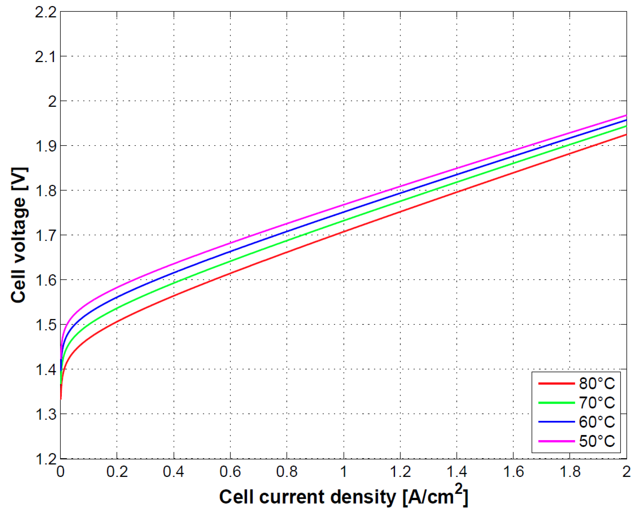
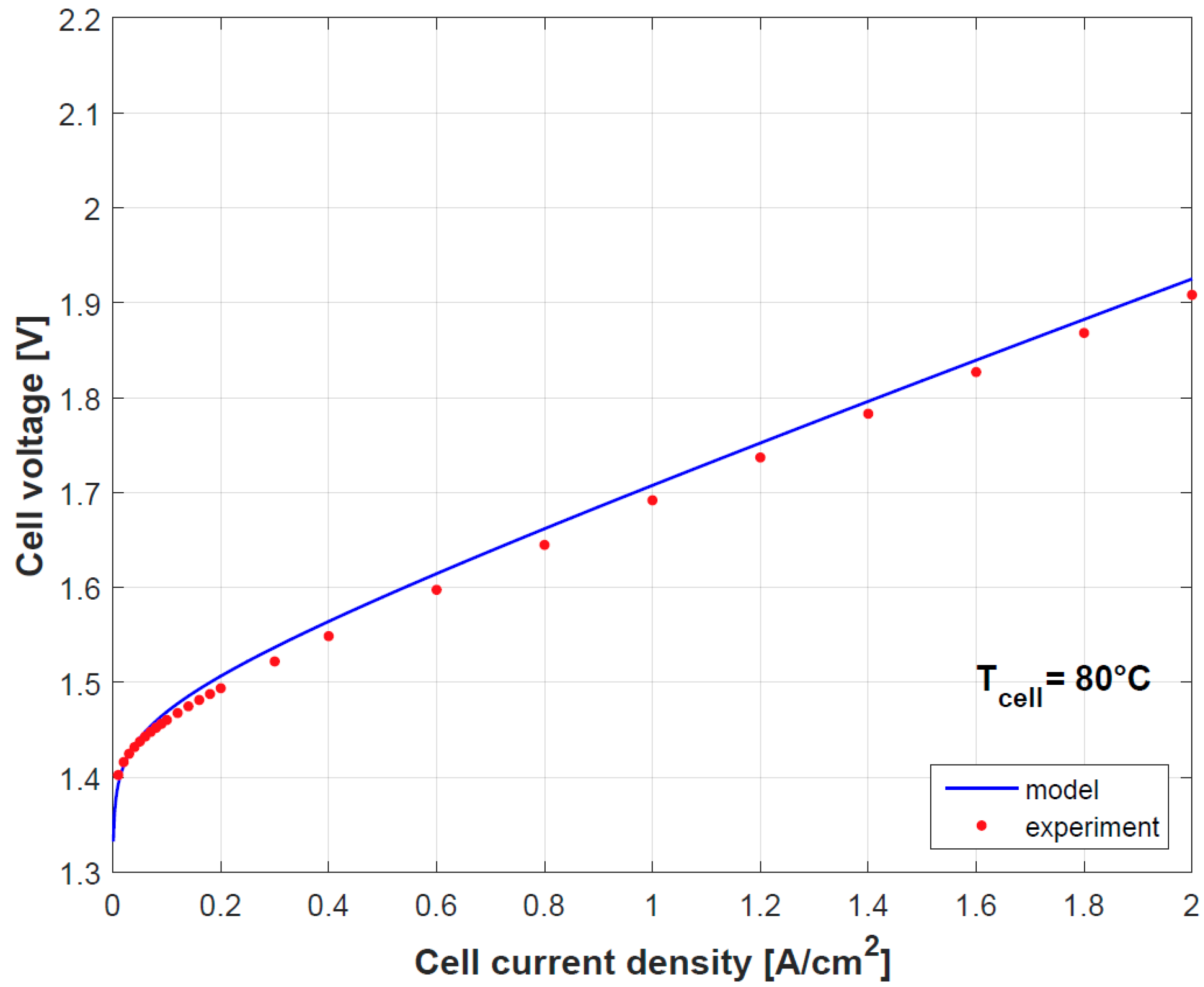
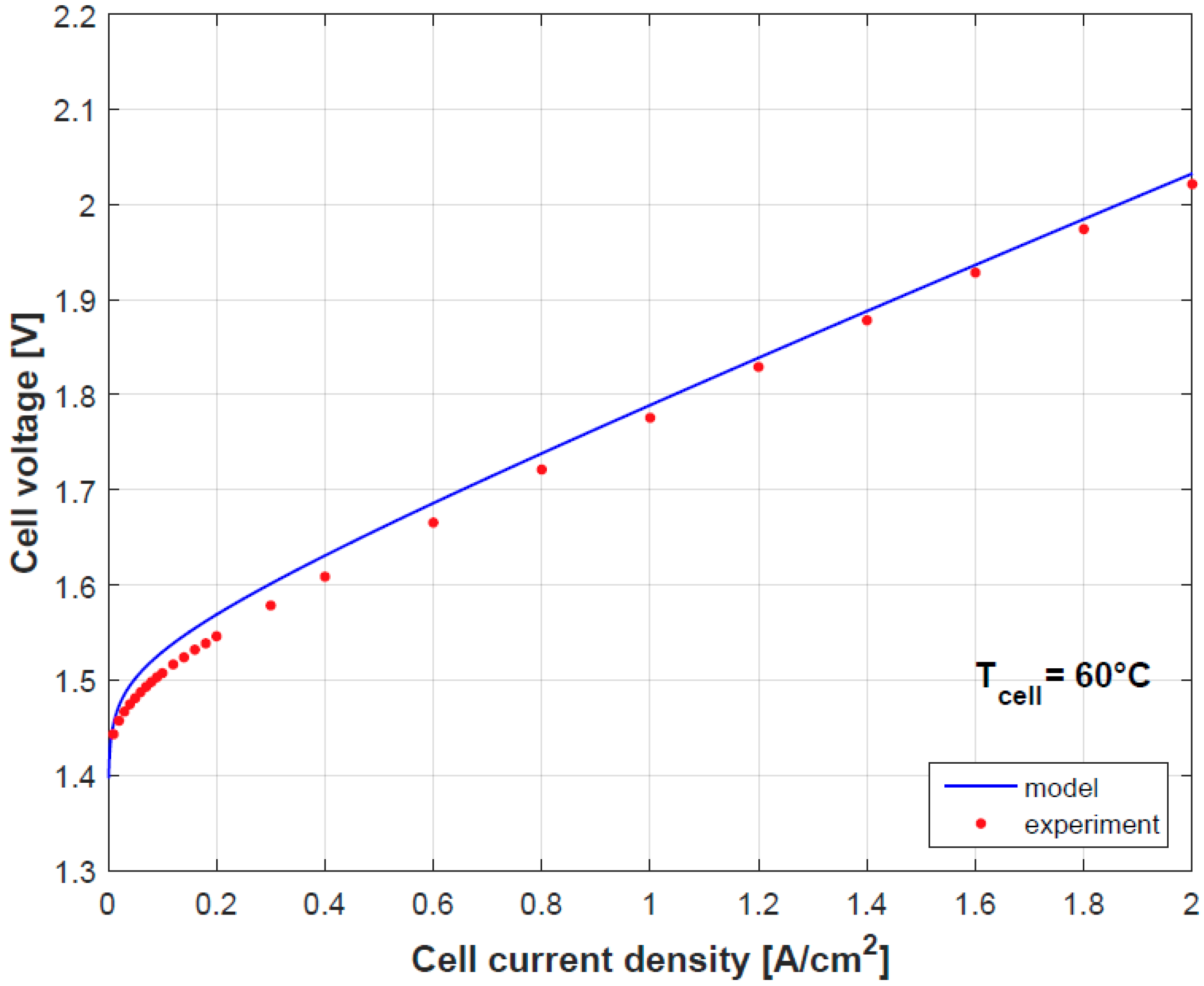
Figure 4 and Figure 5 provide a comparison of the results obtained by both model and experimental tests using the empirically fitted parameters in Table 4. A small discrepancy in the polarization curve is seen due to the model assumption of negligible Ohmic overpotentials in the electrodes and plates, which indeed contribute in limited proportion [9]. Besides as mention before, the temperature dependence of $D_{H^{+}}$ gives a good prediction for the cell performance.

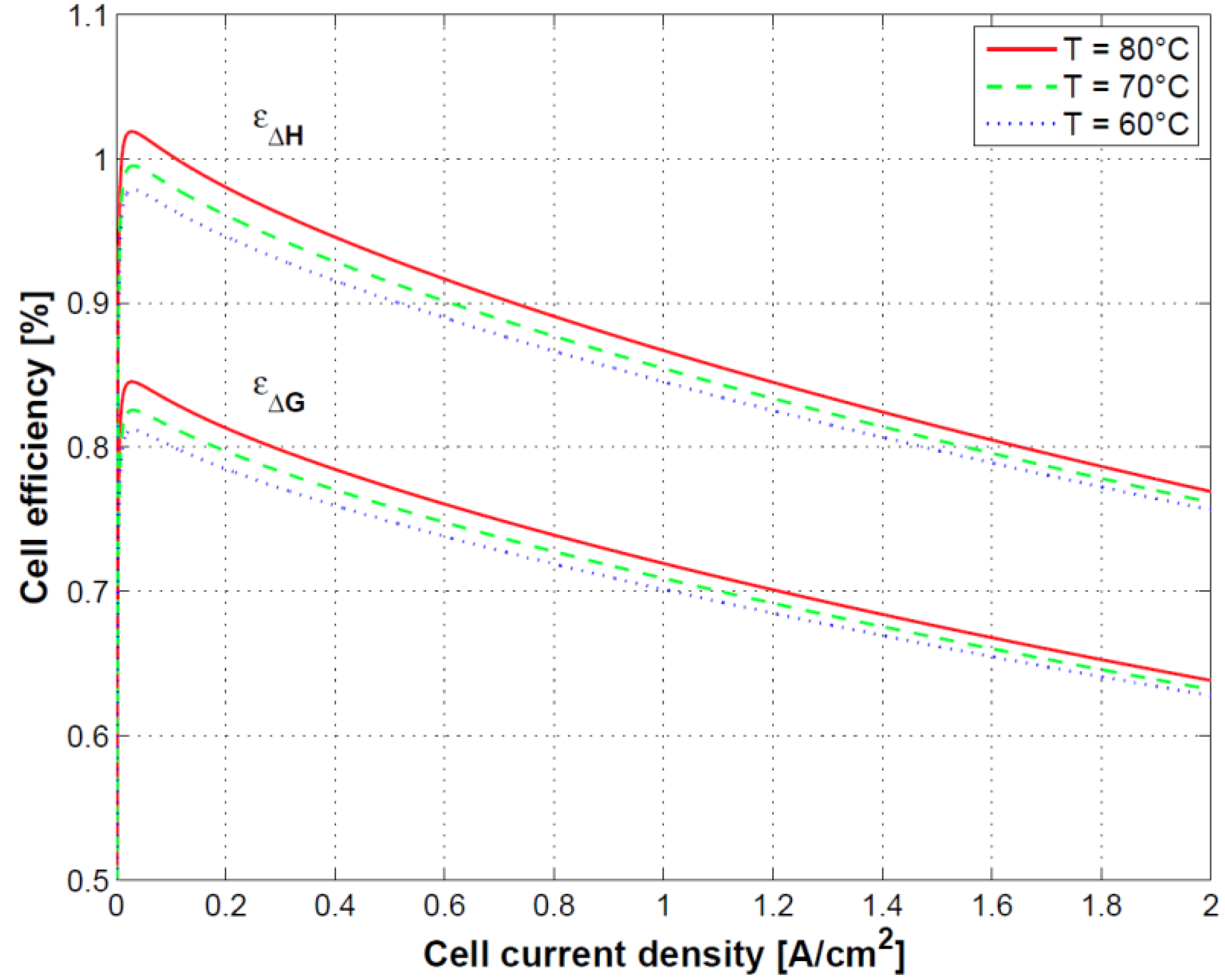
In Figure 6, the effect of temperature on cell performance is depicted. Increasing temperature of operation will reduce the Gibbs free energy of the electrochemical reaction thereby increasing the cell performance and energy conversion. This is in agreement with results provided in [9].

The Ohmic overpotential depends on temperature through the conductivity relationship. This is reflected on a slight increase in the slope of the curves at mid-high current densities.

Figure 7 shows the relatively higher contribution of the anode activation overpotential to the overall activation over potential. The kinetics of the oxygen evolution reaction at the anode side is slower than the hydrogen evolution reaction at cathode side resulting in higher overpotentials at the anode. Nevertheless, the reaction kinetics also depends on physical properties of the electrode material e.g., roughness factor. The charge transfer coefficients at anode and cathode, ${\alpha }_{an}^{}$ and ${\alpha }_{ca}^{}$, gave values similar to those in [9].

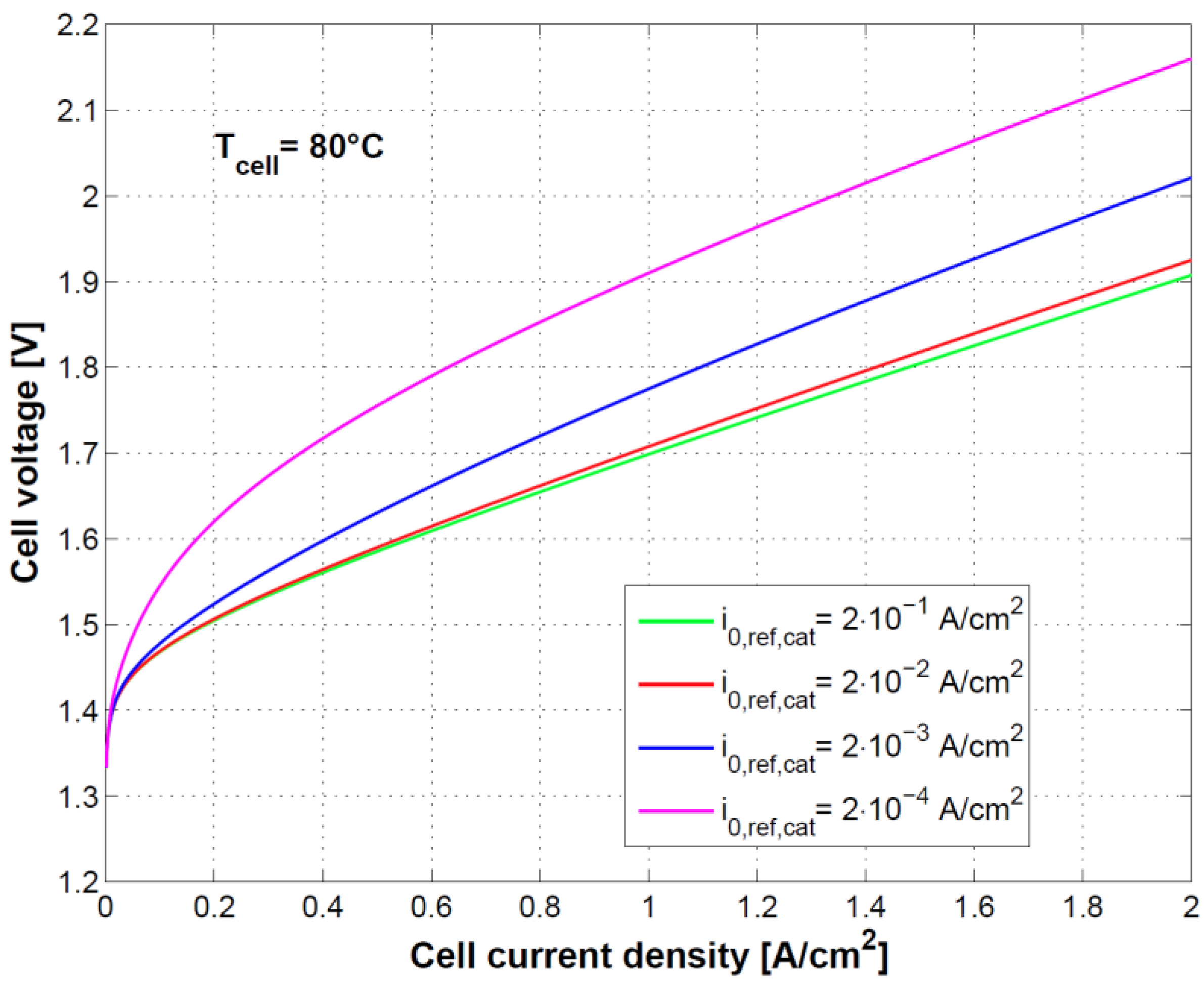
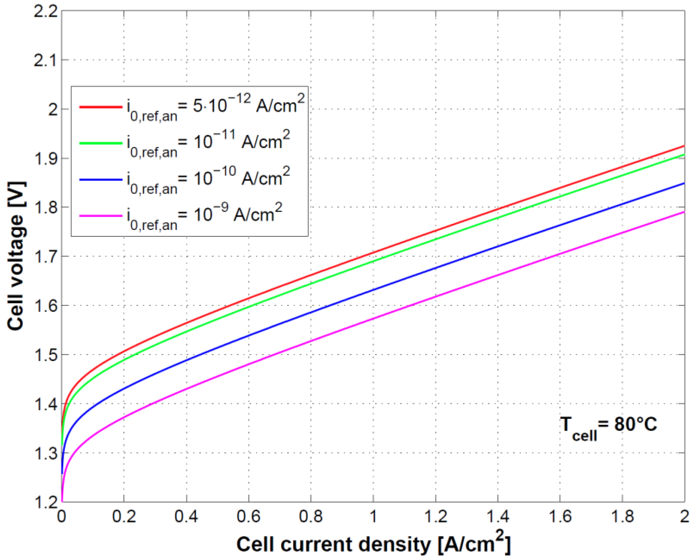
Figure 8 and Figure 9 show the effect of using different exchange current densities at anode and cathode. This parameter mainly affects activation overvoltage as a consequence of different kinetics of charge transfer reactions.

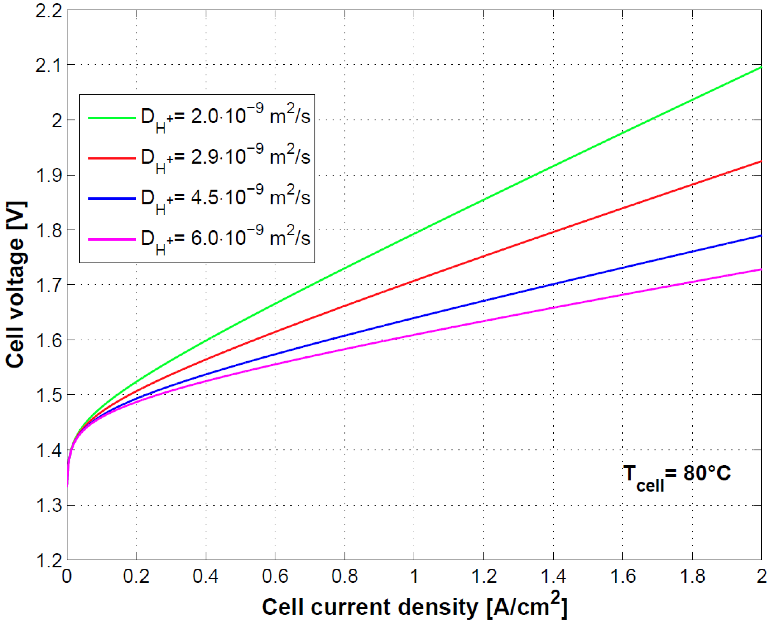
The sensitivity on the cell model to the diffusivity of H⁺ ions is shown in Figure 10. The link of diffusivity of H⁺ ions to membrane conductivity and therefore to ohmic losses is evident as previously shown in Equation (34) and [8].

In Figure 11, the impact of the temperature on the first and second law efficiencies defined in Equations (37) and (39) is shown. First law efficiency can reach values higher than 100% at low current density due to cell heat absorption and strongly reduces with the increase of current density by around 30% over the current density range of operation.

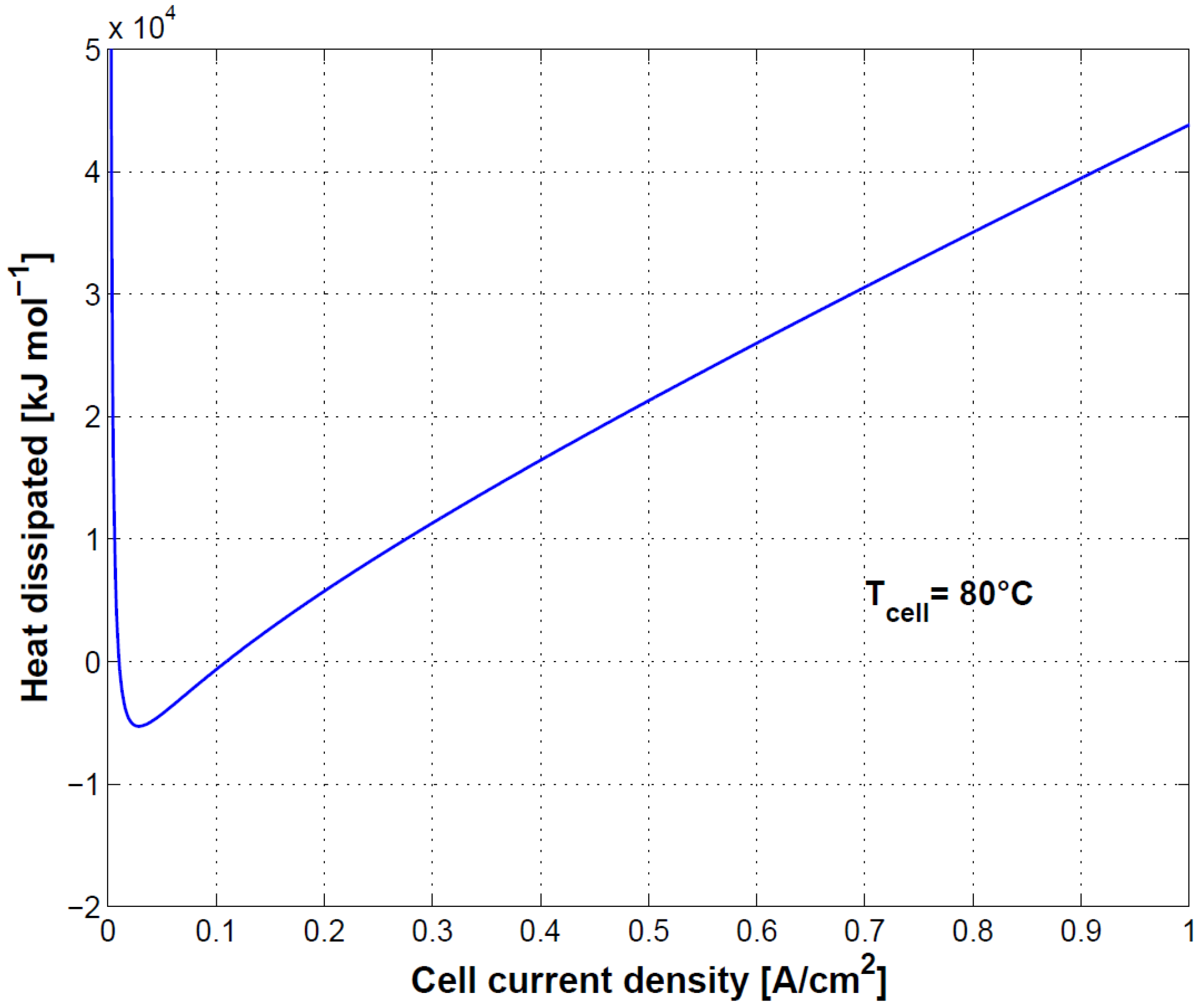
In Figure 12, cell heat loss is shown. At low current density, heat dissipation is negative, meaning that the cell absorbs heat from the surroundings. When hydrogen production is low, the enthalpy change of the electrochemical reaction is higher than the electrical work [23]. At high current density, a high increase in heat dissipation is to be expected.

7. Conclusions

A model of a PEM electrolyzer cell was developed including electrochemical mechanism at the anode, cathode and in the membrane. Cell performance were analyses by defining an efficiency relationship. The model was able to reasonably fit the experimental data at two different temperature values i.e., 60 °C and 80 °C.

In previous studies it has been shown that activation and ohmic over voltages are closely related to temperature. For this reason, key parameters in the overvoltages relationship were chosen for the performance fitting. The electrodes reference exchange current density and electrodes change transfer coefficients showed a sensitivity to temperature; these parameters are related to the activation overvoltage. The hydrogen ion diffusivity is closely related to temperature in the ohmic overvoltage relationship.

Finally, the connection between cell polarization curve, efficiency and heat dissipation was shown. Specifically, because of the heat absorption at low current densities, first principle efficiency can reach values higher than 100%. At high current density efficiency decreases as a result of the reduced performance and related heat dissipation. Oxygen and hydrogen crossover played a less relevant role in this case as the test was conducted at ambient pressure.