1. Introduction
From the previous decades, the energy requirement has grown to a critical level; however, the generation units have not been maintained at a sufficient rate to manage this increasing demand. The balance between demand and generation is a vital requirement for stable power system operation. The problem to maintain this balance has conventionally been addressed in the past; utilities have upgraded their centralized generation units and transmission capabilities through some supply side management methodologies. However, during the previous decade, demand-side management (DSM) has become a substituent scheme to manage the increasing requirement of energy which focuses on the consumer side. The home energy management system (HEMS) is used to implement DSM in a home. Major approaches for HEMS operation include price-based demand response (DR), and DR synergized with renewable energy sources (RESs) and energy storage systems (ESSs) optimal dispatch (DRSREOD) [
1]. The DR-based HEMS operation schedules the consumer’s loads by shifting them towards the off-peak periods. Such scheduling benefits the consumer with a minimized cost of energy (
) based on the acceptable value of time-based discomfort (
) [
2,
3]. The utility, on the other side, is benefited with a reduced cost of generation through a smoother demand profile. The DRSREOD-based HEMS operation schedules the load in coordination with the optimal dispatch of the power grid, renewable energy sources (RESs) and energy storage systems (ESSs). The operation of such HEMS introduces additional benefits by minimizing the electricity cost, minimizing high demands and permanent demands, increasing total cost minimization and empowering the selling of the extra power to the utility [
4,
5,
6,
7,
8,
9,
10,
11]. The aforementioned HEMSs are modeled to optimize the objectives comprising the net
(
), consumer discomfort/inconvenience, and peak and permanent demands. The abbreviations and nomenclature are given in
Table 1 and
Table 2, respectively.
Furthermore, a general architecture of DRSREODLDG-based HEMS is shown in
Figure 1. The main components of such a system include home appliances (HAs), RESs, an ESS, an LDG, the HEM controller (HEMC) and the smart meter (SM) with the local communication for home area network. The SM is used for bidirectional interaction in order to exchange the electricity bill and power consumption data between users and power grid. The HEMC embeds whole computational intelligence which is sufficient for the proposed optimum HEMS operations.
Furthermore, the rampant rise in green house gas (GHG) emissions, the consequent climate changes and the related environmental issues have raised serious concerns over the quality of the life on the earth. In order to mitigate the serious environmental issues, various proposals have been discussed for GHG emissions at the highest international forums to confine them. The Kyoto protocol of United Nations Framework Convention on climate change has been mutually signed by 192 countries all over the world which proposes a reduction in GHG emissions through selling of emission commodities [
12]. Such a trading sets penalties and quantitative limitations on emissions by polluters that may include utilities, independent microgrid (MGD) operators, and the prosumers having fossil fuel based generation deployed with DRSREODLDG-based HEMSs.
The aforementioned scenario has incentivized utilities to reduce not only the cost of generation of energy; however, also the supply-side emissions making use of RESs installed for DRSREOD-based HEMS. The research on HEMS now seems to focus on reducing the GHG emissions along with the other well-known objectives for
,
, etc. In [
13], a scheme for DR-based HEMS is presented. Non-critical house loads are shifted towards low demand periods for minimizing the daily bill of the generation-side and the supply-side emissions. It is validated that implementation of the DR program effectively reduces the cost of generation on the supply-side; however, the emission on this side is reduced only when peak demand is met by high emission fuels based peaking plants. The DRSREOD-based HEMS, on the other hand, through an optimal operation of HEMS devices, can easily be used for reducing the supply-side emissions along with the reductions in the
for the consumer and cost of generation for the utility. In [
14], the authors present a scheme for optimal scheduling of shiftable home appliances (SHAs) integrated with the optimal dispatch of an RES and an storage battery (SB). The objectives include reductions in
, temperature based discomfort, peak load, and the GHG emissions. The supply-side emissions are computed using GHG emission factors (EFTs) for the energy mix adopted at different times of the day. The supply-side emissions are reduced through an optimal operation of local RESs and SBs during high emission times.
Furthermore, fossil fuel based DGs are integrated into MGDs to improve the self-healing structure and the flexibilty of the power supply. In [
15], an operational scheme is developed for a stand-alone HEMS operation using PSO. The scheme is based on load shifting of SHAs, an optimal dispatch of a wind turbine (WTB), a DG, and an SB. The DG is operated at the rated power in order to improve its efficiency and to reduce emissions. The power from the grid, however, is not included in the modeling. In [
16], an optimal dispatch scheme for a PV unit, a WTB, an ESS, a DG, and the power grid to supply a fixed load profile in an MGD is computed using GA. Constraints for ESS charge/discharge rates, generator start/stop and supply capacity are taken into account. Net emission for the power supplied by the grid and local DGs are computed.
Furthermore, fossil-based LDGs are integrated into DRSREOD-based HEMSs to supply the load during load shedding (LSD) hours. Such a LDG adds a vital benefit of uninterrupted supply of power to DRSREOD-based HEMS. An algorithm for optimal sizing of LDG for DRSREODLDG-based HEMS was proposed in our recent research [
11]. The proposed sizing was based on the trade-off analysis for the parameters including
,
and size of LDG. An uninterrupted supply of power through the integration of LDG was ensured; however, the operational schemes for HEMS were remained to be analyzed for the emissions released during the LDG operations. To implement an eco-efficient operation of DRSREODLDG-based HEMS, optimal trade-offs between
,
and minimal GHG emissions
need to be computed. This research introduces a method to harness a diversified set of solutions to decision vector
and the related trade-offs for
,
and minimal
for an eco-efficient HEMS operation.
The proposed method for an eco-efficient operation of DRSREODLDG-based HEMS is based on a three-step approach. In step-1, a set of primary solutions in terms of
and the related trade-offs for
,
and minimal
are generated using Algorithm 1. The algorithm is based on a heuristic derived from our previous studies on HEMS in [
11]. The proposed heuristic takes into account PV availability, the state of charge, the related rates for the storage system and the similar functionality of the sources. To achieve maximum reduction in
, SHAs are modeled for mixed scheduled (MS) as already validated in [
11]. This research formulates the trade-off parameters for:
to include the cost of energy purchased from the grid, cost of energy sold to the grid and the cost of energy supplied by the LDG;
to include the energy supplied by the LDG during LSD hours,
based on the calorific value of the fuel, the consumption efficiency of the LDG and the related emission factors for GHGs; and
to include the delay in the starting times of delay scheduling (DS) type and advanced completion of the job of advanced scheduling (AS) type for HAs. The trade-off solutions obtained in step-1 are analyzed for
as related to the trade-offs between
and
as shown in
Figure 2.
The plot in
Figure 2 reveals a highly un-even relation between
and the related parameters for
and
. This un-even trend for
is exploited to screen out/exclude a set of trade-offs with larger values of
using a constraint filtration mechanism as presented in Algorithm 2 (step-2 and step-3). In step-2, an average value based constraint filter (AVCF) for
is developed and applied to filter out the trade-offs with extremely high values of
. In step-3, average surface fits for
are developed in terms of
and
using polynomial based regression. The most suitable polynomial is selected after cross-validation of 25 number of polynomial model that fits on their capabilities in order to reduce
and
, and to maximize the number of diverse trade-offs for
and
. The average surface fit based constraint filter (ASCF) with the selected polynomial formulation is applied to screen out the trade-offs with even marginally higher values of
. The solutions for an eco-efficient HEMS operation are thus achieved including diversified trade-offs for
,
and minimal
. Followings are the novelties of this research:
An innovative method is proposed to harness diversified trade-offs between , and minimal for an eco-efficient operation of DRSREODLDG-based HEMS.
Trade-offs for such HEMS have rarely been computed by combining a multi-objective genetic algorithm or Pareto optimization (MOGA/PO) based heuristic and regression based constraint filtration. The polynomial model fit for regression is based on its capabilities to reduce the trade-off parameters for eco-efficient HEMS operation.
Most of the authors use the weighted sum method (WSMD) to handle multi-objectivity for similar problems. This research presents a diverse set of trade-offs that are critically analyzed to enable the consumer choosing the best option.
Trends exhibited by the trade-off parameters are analyzed based on vital factors affecting these parameters, e.g., loss of unused energy from the PV unit.
The proposed method validated to minimize the emissions from a local LDG for a DRSREODLDG-based HEMS; however, it is easily extendable to reduce the supply-side emissions as well.
The organization of the paper is as follows:
Section 2 describes the related work whereas the system model is elaborated in
Section 3. The problem formulation for eco-efficient operation of DRSREODLDG-based HEMS and the techniques used to solve this problem are presented in
Section 4. The proposed Algorithm 1 to generate primary trade-offs for optimal HEMS operations, and Algorithm 2 to harness eco-efficient trade-offs through a constraint filtration mechanism are presented in
Section 5. In
Section 6, simulations are presented to demonstrate the validity of Algorithm 1 to generate schemes for DRSREODLDG-based HEMS operation in terms of
and the primary trade-offs between
,
and
. The trends exhibited by the primary trade-offs are analyzed in detail and the bases for the selection of constraint filters including AVCF and ASCF are validated. Further simulations are presented to demonstrate the validity of Algorithm 2 to harness eco-efficient trade-off solutions using the optimal constraint filters. Conclusions and future work are discussed in
Section 7.
2. Related Work
With the installation of smart grid technologies enabling DSM, a widespread deployment of DR- and DRSREOD-based HEMSs has been carried out throughout the world in the past few years [
17,
18]. The report in [
17] has given an overview and boost to the RESs by forming policies among various contries. In [
18], the current phase of Paris agreement has focused on developing a global approach, which limits the GHG emissions of all countries. In recent years, authors have presented various models and methods for the optimal operation of such systems [
2,
3,
4,
5,
6,
7,
8]. The objectives for optimal HEMS operation include minimizing
,
, peak-to-average ratio
and peak/permanent demands [
19,
20,
21]. In [
19], the authors have used different priorities to derive user comfort. Khan et al. [
20] have used three different appliances to minimize
,
, and
. Meta-heuristics approaches including optimal stopping rule are used as optimization schemes. Similarly, the authors in [
21] have applied meta-heuristics approaches along with a hybrid approach to minimize
. Furthermore, utilities owning energy deficient power networks in developing countries are subjecting their users for LSD to maintain energy demand and supply. In such power networks, consumers deploy a LSD-compensating DG in DRSREOD-based HEMS for ensuring the reliable distribution of the energy [
11]. The aforementioned objectives for optimal HEMS operation have been achieved using optimization techniques like linear programming (LP), mixed integer LP (MILP), advanced heuristics, etc.
Additionally, the issue regarding serious environmental concerns over the use of fossil fuels has been raised at international forums consistently in the past few decades. Recently, worldwide consensus has been reached to reduce the GHG emissions by selling them as commodities [
12]. Such trading sets quantitative limitations on the emissions made by polluters that may include utilities, independent MGD operators and the prosumers having local fossil fuel based generations. The present scenario based on the polluter pays principle has incentivized utilities to reduce not only the generation cost; however, the supply-side emissions as well while making use of the RESs installed for DRSREOD-based HEMSs [
14,
22,
23]. Furthermore, MGD operators having RESs, ESSs and DGs also include
as an objective in the optimal dispatch scheme for their systems [
15,
16,
24]. Furthermore, in energy-deficient power networks, DRSREODLDG-based HEMSs having LSD-compensating DGs are used to ensure an uninterrupted supply of power during LSD hours [
11]. The operation of LDG in such HEMSs, however, does accompany the release of emissions, which needs to be minimized.
The related work includes the recent research on models and methods to achieve important objectives for DR and DRSREOD-based HEMSs including reductions in
(supply-side),
, and
; for MGDs including reductions in
and
; and for DRSREODLDG-based HEMS including reductions in
(local),
and
. The recent research related to the proposed method for an eco-efficient operation of DRSREODLDG-based HEMS is summarized in
Table 3 and
Table 4.
2.1. Emissions Reduction Using DR-Based HEMSs
Most of the research on DR-based HEMS has focused on objectives like
,
, peak load and discomfort [
2,
3]. Such systems have limited capabilities to play a role in the reduction of GHG emissions. In [
13], a scheme for DR based HEMS is presented. Non-critical house loads are shifted towards off-peak hours to minimize the daily cost of generation and emissions for the supply-side. It is validated that implementation of DR program effectively reduces the cost of generation on the supply-side; however, the emissions on this side are reduced only when peak demand is met by peaking plants based on high emission fuels like coal, diesel, etc.
2.2. Emissions Reduction Using DRSREOD-Based HEMSs
Most of the models for DRSREOD-based HEMS presented in the recent past are based on optimal scheduling of SHAs integrated with the optimal dispatch of RESs and ESSs. HEMS problems for these models have been solved to reduce
and discomfort for the consumer, and to minimize peak load/PAR and cost of generation for the utility [
4,
5,
6,
7,
8]. Recently, in the context of worldwide concerns over GHG emissions, authors have focused on the reduction in emission as an objective for DRSREOD-based HEMS. In [
14], authors proposed a scheme for optimal scheduling of SHAs integrated with the optimal dispatch of RES, SB, and the utility. Major goals include reductions in
, temperature based discomfort, peak load, and the supply-side emissions. Such emissions are computed using emission coefficients for the energy mix adopted by the utility during various times of the day. An optimal dispatch of local RESs and SBs results in the reduction of net supply-side emissions by supplying the load during high emission hours. MILP has been used to solve the model. In [
22], an operating mechanism of major HAs including heating and cooling appliances integrated with the optimal dispatch of PV and SB is presented. The algorithm for real-time HEMS operation is based on user preferences, home occupancy, day ahead emissions and climate forecasts. The objectives for reduction in
, electric consumption,
, and the peak demand are formulated. The net cost of emission includes carbon footprint of the customer from the grid electricity usage minus carbon reduction from injecting emission-free electricity from RES. In [
23], a prosumer based algorithm is presented to maximize the sum of benefits to the consumer and the utility. The emission trading has been considered as a mean of mitigating this commodity. The utility is profited by reducing his carbon footprints while purchasing energy from locally installed RESs and ESSs during high emission times. The fitness function maximizes the welfare including consumption-based satisfaction and monetary benefits from RESs and ESSs to consumers and benefits of the reduced peak load, generating cost and emissions to the utility. A dynamic selling with dynamic buy-back pricing scheme is also proposed to implement the model. For scalability and user privacy, the problem is solved using Lagrange multipliers. The objectives in all of the above research are combined using the WSMD.
2.3. Emissions Reduction in MGDs
In MGDs, RESs and ESSs are integrated with DGs to enhance the quality and the reliability of the power supply. In [
15], a solution for DRSREOD-based HEMS operations for a stand-alone home including WTB, DG, and SB is computed using PSO. The local fossil fueled DG is operated at rated power for an improved efficiency and reduced emissions. A separate objective function for emissions; however, is not included. An optimal dispatch for an MGD is computed in [
16] using GA. Additional constraints for ESS charge/discharge rates, DG start/stop and supply capacity are considered. Total emission is computed using emission factors for the grid, power supplied from the local DG and the ESS. The model does not include load shifting while computing the dispatch for power sources. A method to compute an optimal dispatch of RESs and DGs for a MGD is presented in [
24]. The dispatch is based on costs of energy from WTB, PV and DG,
and
from/to main grid for a fixed load profile. The WTB and the PV are the preferred sources. The SB is discharged based on its SoC if local RESs are not able to meet the demand; else, the load is supplied through the economic dispatch of the DG, fuel cell (FC), SB and the grid. Non-critical loads are disconnected when local sources are insufficient. The DG is operated at rated power to minimize
. DR based load shifting is not included.
2.4. Emissions Reduction in DRSREODLDG-Based HEMS
Energy-deficient power supply networks in developing countries are based on the compromises for the consumers to LSD in order to maintain the equilibrium between demand and generation of energy [
10,
11]. While a number of consumers in developing countries are participating in DSM making use of DRSREOD-based HEMSs, LSD-compensating DGs are deployed in such HEMSs for ensuring the uninterrupted supply of electricity. An algorithm for optimum sizing of an LDG for DRSREOD-based HEMS was presented in our recent research [
11]; however, such a DG does introduce emissions when operated during LSD hours. Based on the recent scenario for quantitative restrictions on carbon emissions, research on the optimized operation of DRSREODLDG-based HEMS focusing reduction in
looks pertinent. A simulation-based posteriori method for an eco-efficient operation of DRSREODLDG-based HEMS takes into account the trade-offs between
,
, and minimal
is proposed. A three-step approach is followed. At step-1, primary trade-off solutions for
,
, and
are generated using a heuristic proposed for an optimal operation of DRSREODLDG-based HEMS. The heuristic, which uses MOGA/PO to search optimal trade-offs, is detailed in Algorithm 1. At step-2, an AVCF is used to filter out the trade-offs with extremely high values of
, whereas an ASCF is used to screen out the trade-offs with marginally high values of
at step-3. The ASCF was developed using advanced regression techniques. The filtration mechanism including AVCF and ASCF used to harness eco-efficient trade-off solutions for
,
, and minimal
is detailed in Algorithm 2.
3. System Model
The architecture for DRSREODLDG-based HEMS is shown in
Figure 1. The major components of such HEMSs include home appliances, renewable energy sources, an energy storage system, an LSD-compensating DG, a HEMS controller, a local communication network, and a smart meter for bidirectional interation between users and the power grid. The proposed optimal operation for such HEMS are based on DR synergized with the optimal dispatch scheme for RESs, ESSs and an LDG. The operating scheme takes into account the MS of SHAs, their combined corresponding functions of the PV unit, the SB and the utility, and the energy sold to the grid based on the parametric values of power vector from PV
, vectors of the state of charge
, the maximum charge/discharge rates, and the tariff scheme. PV unit is the preferred source that is responsible for suppling the power to the scheduled appliances. The surplus PV energy is saved into the SB for utilizing the power during peak hours and it is sold to the utility for a monetary benefit. During the LSD hours, if SB is full and there is no energy demand than the excess energy from the PV unit is dissipated in a dummy load [
9]. The mentioned energy (shown by
) represents a loss of the PV energy that could not be sold due to the unavailability of the main grid. The LDG is used for supplying the load in high demand periods which is contributing similar to PV unit and the SB to prevent the electricity blackouts. The operation of the LDG in such systems ensures an uninterrupted supply of power; however, such operation of the LDG accompanies the release of GHGs emissions as well. The problem for DRSREODLDG-based HEMS operation has been formulated as multi-objective-optimization (MOO) to minimize
,
, and
.
Furthermore, according to [
10], 31% and 21% energy is consumed in industrial and residential sectors, respectively. However, in this paper, we consider only residential area for implementation of our proposed scheme. Because our proposed schemes are based on load scheduling from ON-peak to OFF-peak hours, it is not possible in industrial or agriculture sectors to reduce electricity cost via load shifting due to production problems. Therefore, we consider only residential area for implementations. Moreover, there are a lack of sources in developing countries, so the energy management system is a huge opportunity for these countries.
A three-step simulation based posteriori method is proposed to provide trade-off solutions for an eco-efficient operation of DRSREODLDG-based HEMS. The method makes use of Algorithm 1 and Algorithm 2 to harness eco-efficient schemes for HEMS operation in terms of
and the related trade-offs for
,
, and minimal
. At step-1, primary trade-off solutions for
,
, and
are generated making use of Algorithm 1. Algorithm 1 is based on a MOGA/PO based heuristic proposed in this work. At step-2, the primary trade-off solutions are passed through an AVCF to filter out the trade-offs with extremely high and above average values of
. The filtrate is then passed through an ASCF to screen out the trade-offs with even the marginally higher values of
at step-3. The proposed filtration mechanism comprising AVCF and ASCF is detailed in Algorithm 2. The simulations to validate the method for harnessing the desired trade-offs for eco-efficient operation of DRSREODLDG-based HEMS are presented in
Section 6.
Major components of the proposed model for DRSREODLDG-based HEMS are presented below.
3.1. Parameters for Scheduling
A scheduling resolution of 10 min. slot has been adopted. To formulate the HEMS operations, total time is sub-divided into 144 slots. While scheduling, each SHA is executed in the specific horizon for a specified number of slots. The proposed model for HEMS operation is dependant on a dynamic electric pricing signal, i.e., an IBR pricing signal, the PV panel, the SB, and the LDG. The control parameters for HEMS components are described in
Section 4 on problem formulation.
3.2. HAs
Motivated from the literature [
21,
25], the HAs are classified into non-shiftable home appliances (NSHAs) and SHAs. NSHA, e.g., electric lamps, and fans, are working on required time slots and can not be opted for scheduling. SHAs are assumed to be scheduled towards the low demand hours and the PV harnessing hours for optimized HEMS operation. To achieve a maximized reduction in the cost of energy, shiftable appliances are modeled as AS and DS. Such classification enables more reduction in the cost of energy making use of enhanced flexibility in the appliances shifting and an increased direct usage of the PV energy from the PV unit [
11]. AS and DS type SHAs with the user prioritize settings and the NSHAs along with their forecasted load, used in the simulation section are described in
Table 5 and
Table 6.
The proposed method is generic in nature and is equally applicable to DRSREODLDG-based HEMS based on time-of-use pricing and Day-ahead pricing schemes. A 2-step ToU pricing tariff with respective IBR values and threshold power demand are used in simulations in
Section 6.
3.3. RESs
Solar irradiation data as measured by the Pakistan Engineering Council in Islamabad has been applied for the simulations to validate the proposed system [
11]. It is possible to sell the surplus energy produced from the RESs [
26]. The PV system is used in the simulations and its parameters’ configurations are given in
Table 7. The energy generation profile of PV unit is displayed in
Figure 3. The electricity bill of generations from local RESs has not been included in the model and such installations have been considered as a module of the current system [
11].
3.4. ESS
The SB and the inverter are important parts of the proposed DRSREODLDG-based HEMS. These components along with their specifications are given in
Table 8. Net loss for the SB is initially supposed up to 20%; otherwise, it is considered for charging.
3.5. LDG
The consumers perform optimally sizing the LDGs according to their deficient load as [
27]. The specifications of the LDG to cope with the LSD are used in the simulation of proposed model as given in
Table 9. The emission factor is computed as per Equation (
8) using the pertinent data given in [
28,
29]. The cost of energy for the LDG is according to the levelized cost of energy for such units given in [
30].
4. Formulating DRSREODLDG-Based HEMS Problem and the Related Optimization Techniques
The contents of this section are inherently divided into two parts: (1) the problem formulation for HEMS optimization to generate optimal schedules of SHAs in terms of and the primary trade-offs for , and along with the proposed techniques.
The problem to generate the primary trade-offs for , and is computed using the following input values:
= SHAs used for scheduling,
= Slot numbers defined for the scheduling horizon,
= Power ratings of the SHAs rer-slot,
= SHAs having different lengths of operation time,
= SHAs starting slots,
= SHAs Ending slots,
= ToU pricing tariff values in Cents/kWh,
= factors for power more than ,
= Each SHA’s decision vector for start time.
The problems for HEMS are formulated to compute the power requirement for whole of the scheduling horizon. With
as the decision vector, HEMS problem for the scheduling vector
is treated as MILP and computed using the following Equations.:
where
for the
SHA is computed based on the following terms,
The load vector
for NSHAs is added to
to calculate the final scheduled load vector
using Equation (
2):
The problem is solved using a MOGA/PO based heuristic proposed in Algorithm 1 to obtain a decision vector, , which optimizes the outcomes for trade-offs parameters by fulfilling the required constraints.
4.1. Objectives for DRSREODLDG-Based HEMS Problems
The main objective for DRSREODLDG-based HEMS optimization is to achieve the optimal trade-offs between the , and . To obtain the above-mentioned trade-offs, the problem for HEMS is formulated using SHA schedules by calculating paralelly, synergizing the scheduling with RES, ESS, LDG and power grid dispatch for N time intervals over a specified scheduling horizon. The LDG is integrated in the dispatch only for the LSD intervals to supply the load in collaboration with the PV unit and SB. The heuristic presented in Algorithm 1 computes the corresponding vectors for , , and that are used to compute the objective functions/trade-off parameters.
4.1.1. Reduction of
The
is computed using the Equation (
5):
Here, and are the power purchased from the main grid and its price in Cents/kWh. The terms and are the energy sold to the utility by the consumer and its feed-in price in Cents/kWh, respectively. and are the energy supplied from the LDG and its levelized price in Cents/kWh, respectively. A factor can be excluded from as a reward for reducing the supply-side emissions through the PV energy sold to the utility.
4.1.2. Minimization of for the Consumer
We consider user discomfort in terms of average waiting time (TBD) of appliances. It simply means how much time a user will wait to switch ON any appliance. Moreover, the maximum average waiting time means maximum user discomfort and vice versa. For instance, if the average waiting time of all appliances is four hours, then user discomfort will increase by 0.4 because the user feels discomfort to wait. Moreover, in the case of unscheduled electricity consumption, users do not wait to turn ON their appliances. Electricity user can use any appliance at any time, so their waiting time is 0 and the user’s comfort is maximum (no discomfort). The
formulation is given below:
where
and
indicate the users’ time bounds flexibility for representing the starting and ending boundaries for SHAs working.
is a vector which is comprised of total length of operation time for eacg SHA for completing its execution.
is also a decision vector which consists of starting intervals of all SHAs, whereas
is the number of SHAs designated as DS.
When the corresponding SHA starts its execution at
, the
uses its initial value as 0, i.e., the start of the execution time is assigned from the users. When
is equal to
+ 1, it obtains its maximum value at 1, i.e., late starting time for the SHA results in finishing of the task at the late alloted time
. The boundaries for the selection of
should be considered feasibly which are calculated with the help of the next Equation:
Due to the advanced completion of the jobs of AS type SHAs denoted by
, the average
is computed. It is calculated by taking the average of the normalized advance-completion times of all gadgets. This value is computed using the next equation:
whereas,
denotes the number of SHAs for AS type.
When the corresponding SHA completes its execution at , takes its initial value as 0, for example, when -1 is equal to . When is equal to , it gets its maximum value as 1, for example, using the finishing time of the appliance which is calculated with − 1.
There are muitple appliances and some of them are categorized as AS and others are categorized as AS in MS. For minimizing the average
for total
k appliances in MS mode, the objective function is defined as below:
For a scheduling flexibility and better reduction in
,
based on MS of SHAs as per Equation (
7) has been opted for this model.
4.1.3. Reduction of
Equation (
8) computes the emissions’ minimization ratio, i.e.,
, from which the LDG is formulated:
Here,
is the carbon emission factor (kg/kWh) and
is the vector for the energy supplied by the LDG in kWh during the LSD hours [
13,
16]. A value of 1.6 Lbs./kWh has been used for
for the LDG as per the data available in [
28,
29].
4.2. Techniques to Solve DRSREODLDG-Based HEMS Optimization Problems
The HEMS optimization is considered as a combinatorial optimization problem. Multiple HEMS problems are nonlinear, non-convex constrained, multi-dimensional in nature and they have a variety of the solutions available in literature. To solve these problems, both conventional and advanced heuristic optimization techniques are used.
4.3. Techniques to Handle Multi-Objectivity in HEMS Optimization
Multiple HEMS optimization problems faced in existing scenarios are multi-objective optimization (MOO); however, these problems have conflicting objectives. Minimization of
is considered as a major aim in most existing studies on HEMS, while minimizing
is another significant aim in the consumer perspective. After the serious concerns over the environmental issues, the role of DRSREOD-based HEMS to reduce the emissions due to the local as well as due to the centralized generation by the utility has recently started to be investigated. Various methods have been used in the recent research to take into account important trade-offs between
,
and
. The most widely used approach is the WSMD [
12,
13,
15,
18,
19,
20]. This is an a priori technique that converts MOO into single-objective optimization (SOO) in order to achieve one solution. These techniques do not give the feasible relations among the objectives to allow the consumer to choose among specific preferences. The methods may miss a number of good solutions for a specific user regardless of their preference standards. Analysis of the trade-offs among the above-mentioned aims is considered very pertinent, which enables consumers in decison-making from the set of the diverse set of optimized outcomes. The posteriori method known as Pareto-based multi-objective optimization is dependent on the Pareto dominance idea, which provides the diverse set of possible solutions for multiple objectives.
The concept of MOO problems for a HEMS using decision vector
and
m objectives for Pareto-based optimization is computed as: minimizing the objective vector
, following the mentioned constraints. When
is better than
in any one of the given objectives and is not considered worse in any other than the solution
, which is said to dominate another
. The Pareto-optimal set is composed of the set of non-dominated solutions. The recently introduced MOGA includes features to implement Pareto optimization. Pareto-optimal sets providing optimal trade-offs between
,
and
for a DRSREODLDG-based HEMS have been calculated in this work by using MOGA and the Pareto optimization features as described in Algorithm 1. One hundred of these aforementioned trade-offs computed through MOGA/PO based heuristic are processed to enhance eco-efficiency making use of a constrained filtration mechanism as discussed in
Section 4.4 and
Section 4.5.
4.4. Constrained Filtration of Trade-Offs to HEMS Optimization
The trade-off solutions achieved for a multi-objective optimization problem can be passed through an adequately designed filtration mechanism in order to apply a constraint on any one or more of the specified trade-offs. Such filtration mechanism enables harnessing the trade-offs with enhanced efficiency. In this research, a filtration mechanism has been proposed to screen out the trade-offs with larger values of
as related to the trade-offs for
and
. This mechanism comprises of an AVCF and an ASCF. AVCF makes use of an average value of the trade-off parameter
to filter out the trade-offs with above average and extremely high values of
. While ASCF takes into account an average surface fit for
in terms of
and
to screen out the trade-offs with higher values of
. ASCF has been developed using polynomial based regression technique elaborated in
Section 4.5. The formulation for AVCF and ASCF and their application to harness eco-efficient trade-off solutions are presented in
Section 4.
4.5. Regression Based Surface Fitting Techniques to Develop ASCF
Regression models are used to establish a relation between the dependent and the independent variables in a set of data (
,
,
). In order to develop a surface for the variable
z in terms of variables
x and
y, a regression model is fit to the set of input data. Major models for surface fitting include interpolant, lowess, and polynomial. A polynomial surface fit model has been used in this research for its flexibility in application to the input data. For polynomial surfaces, a general model is designated as Poly(
), where
k is the degree in
x and
l is the degree in
y. The degree of
x in each term will be less than or equal to
k, and the degree of
y in each term will be less than or equal to
l. The maximum for the sum of
k and
l is
m. The degree of the polynomial is the maximum of the values of
k and
l. A linear regression model (LRM) for
i number of observations for the independent variables (
,
) defines a curved surface for the dependent variable
in a 3D-space. The LRM for the surface in terms of an order-
m polynomial may be represented as:
where
.
is called a dependent variable or regressand, and
and
are called independent variable or regressors. The first term in Equation (
9) is deterministic and represents the conditional mean of
based on the given values of
and
. The second term
, called the error term, is random in nature. The term is added or subtracted from the first term to realize the actual data.
are called regression coefficients (RCs). In LRMs, they are assumed to be fixed numbers. The term linear in LRM refers to the linearity of the RCs. The fitting of a model is based on the estimates for the RCs. The estimation is carried out based on the minimization of the least squares of the error term called a least square method. Based on Equation (
9),
is the difference between the actual value of
and the one obtained through the regression. For an optimal linear coefficient (LC) for surface fitting, the sum of the squared error term (
) to be minimized is given as follows:
As
is a function of RCs, the minimum value of the
may be computed by taking partial derivatives of the same with respect to each of the RCs and equating the expression to zero. Based on the estimated a(
), a sample model
is formulated and the error term is also known as residuals, which is computed as
. The regression coefficients
are the estimators of
and
is the estimator of the error term
. The numerical values taken by an estimator are called estimates. The least-squares solution to the problem is a vector
, which estimates the unknown vector of coefficients
. In present research,
has been used to estimate the model fit for an average surface for
in terms of
and
. It is assumed that the observed data is of equal quality and thus has constant variance; however, the fit might be unduly influenced by the data of poor quality. Methods like weighted-least-squares regression are applied to reduce the influence of the low quality data on estimating the model fits [
31,
32]. In present research, the use of AVCF to screen out the trade-offs with extremely high values of
inherently improves the data quality for the model fit for ASCF.
The model fit in this research is based on minimization of
that may be improved using methods like minimization of root mean square error and root mean square error of approximation. However, the improved well-fitting is of minimal value, if it is not based on the ideas from a theory validation point of view and in such cases an extensive cross-validation is required [
33]. Accordingly, various polynomial models fit, 25 in number, have been examined for their capabilities to reduce the average value of trade-off parameters for
and the number of diverse trade-offs available for
and
after the application of filtration mechanism.
5. Algorithms for Eco-Efficient Trade-Offs for DRSREODLDG-Based HEMS
A three-step approach has been used to achieve eco-efficient trade-off solutions for DRSREODLDG-based HEMS. In step-1, schemes for optimal HEMS operation and the related trade-offs for , , and are computed using Algorithm 1. The trade-off solutions thus obtained are passed through a filtration mechanism to harness the ones with bare minimum in terms of and using Algorithm 2. The filtration mechanism is completed in two stages designated as step-2 and step-3. In step-2, an AVCF for is developed and applied to the primary trade-offs to filter out the ones with extremely high and above average values of . The remaining trade-offs are then passed to step-3 to screen out the trade-offs with even the marginally higher values of . In step-3, an ASCF is used to filter out the trade-offs with parameters residing above the average surface fit for . Eco-efficient solutions including bare minimum and diversified trade-offs for and are thus achieved for DRSREODLDG-based HEMS operation. The followings algorithms have been proposed to harness the eco-efficient tradeoff solutions for DRSREODLDG-based HEMS:
The algorithms are presented in the following subsections.
| Algorithm 1: Algorithm to generate operating schemes and the primary tradeoffs for drsreodldg-based hems (step-1). |
Input: , , , , , , , , , , , , , , , , , ,
Output: Optimal tradeoffs for , and with for SHAs
1: Initialize input parameters
2: Call MOGA
3: Initialize Tst within bounds STslot and ENslot-LoT+1
4: for Iterat = 1: Ng_mx
5: if Iterat > 1
6: Generate new Tst populations within bounds using GA operations
7: end
—-Computing vector for DR-based scheduling—–
8: Tend = Tst+LoT-1
9: for i = 1:k
10: for j = 1:N
11: if
12: Power_matrix(i,j) = Pa(i)
13: else
14: Power_matrix(i,j) = 0
15: end
16: end
17: end
18: Pschd = sum(Power_matrix)+ Pload_nsh
—–Computing dispatch for the PV system, SB, grid and the LDG—–
19: for j = 1:N
20: Pres(j) = Ppv(j)-Pschd(j)
——-Dispatch when PV energy > Pschd——-
21: case (Ppv(j) > Pschd(j)) do
22: if SoC(j) ≥ SoC_mx
23: if Pgds(j) == 0
24: Pdl = Pres(j)
25: else
26: Psold(j) = Pres(j)
27: end
28: SoC(j+1) = SoC(j)
29: else
30: Pch(j) = min(Pch_mx,Pres(j),SoC_mx-SoC(j))
31: if Pch(j)≠ Pres(j)
32: if Pgds(j) == 0
33: Pdl = Pres(j)-Pch(j)
34: else
35: Psold(j) = Pres(j)-Pch(j)
36: end
37: end
38: SoC(j+1) = SoC(j)+0.8* Pch(j)
39: end
40: endcase
——-Dispatch when PV energy ≤ Pschd——-
41: case (Ppv(j)≤ Pschd(j)) do
42: if (SoC(j)≤ SoC_mn) ((SoC(j)> SoC_mn) && (PE(j)≤ price_set))
43: if Pgds(j) == 1
44: Pgd(j) = -Pres(j)
45: else
46: Pgn(j) = -Pres(j)
47: end
48: SoC(j+1) = SoC(j)
49: elseif ((SoC(j)> SoC_mn) & & (PE(j)> price_set))
50: Pds(j) = min(Pds_mx,-Pres(j),SoC(j)-SoC_mn)
51: if Pds(j) == Pds_mx
52: Pload_d(j) = Pschd(j)-Ppv(j)- pds_mx
53: elseif Pds(j) == (SoC(j)-SoC_mn)
54: Pload_d(j) = Pschd(j)-Ppv(j)-(SoC(j)-SoC_mn)
55: end
56: if Pgds(j) == 0
57: Pgn = Pload_d(j)
58: Pload_d(j) = 0
59: end
60: SoC(j+1) = SoC(j)-Pds(j)
61: end
62: endcase
63: Pgd(j) = Pgd(j)+Pload_d(j)
——-Computing tariffs with ———
64: if Pgd(j)> TP
65: PE(j) = IBR × PE(j)
66: end
67: end
—–Computing fitness function for —–
68: = EFT × sum(Pgn)
—–Computing fitness functions for —–
69: CEnet = sum(PE × Pgd)+sum(PEg × Pgn)-sum(PEf × Psold)
—–Computing fitness function for —–
70: for a = 1:k
71: if Styp = DS
72: (a) = (Tst(a)-STslot(a))/(ENslot(a)-LoT(a)-STslot(a)+1)
73: else
74: (a) = (ENslot(a)-Tst(a)-LoT(a)+1)/ (ENslot(a)-LoT(a)-STslot(a)+1)
75: end
76: end
77: Compute = (sum(TBD(D))+sum(TBD(A)))/k
78: end
79: Exit MOGA; return results as , and tradeoffs and corresponding
80: Goto Algorithm 2 to harness eco-efficient tradeoff solutions |
| Algorithm 2: Algorithm for filtration mechanism to harness eco-efficient tradeoffs for drsreodldg-based hems (step-2 and step-3). |
Input: Tradeoffs from algorithm 1 for , and
Output: Eco-efficient tradeoff solutions for , and minimal
—–Step-2: Filtration of tradeoff solutions using AVCF for —–
1: Do
—–Computing average value of —–
2: TEMiss_avg = Average (TEMiss)
—–Computing residuals for w.r.t —–
3: TEMiss_Resid_avg = Average (TEMiss)- TEMiss
—–Filtration based on average value of —–
4: Filter out/ Exclude solutions with negative TEMiss_Resid_avg
5: Collect the remaining solutions for refined filtration in step-3
6: End do
—–Step-3: Refined filtration of tradeoffs based on average surface of —–
7: Do
8: Tabulate CEnet, TBD and TEMiss
—–Computing average surface for —–
9: Generate an average surface using polynomial option (Ploy41)
—–Computing residuals for w.r.t average polynomial surface—–
10: TEMiss_Resid_avgs = TEMiss on surface - Actual value of TEMiss
—–Filtration based on average surface of —–
11: Filter out tradeoffs with negative TEMiss_Resid_avgs
12: Collect the remaining tradeoffs as eco-efficient tradeoff solutions
13: End do |
5.1. Algorithm 1 to Generate Operating Schemes and the Primary Tradeoffs for DRSREODLDG-Based HEMS (Step-1)
This algorithm computes a set of primary tradeoff solutions for optimized HEMS operation based on MS of SHAs synergized with the optimal dispatch of the PV system, the SB, the grid, and an LDG. The LDG supplies the load only during LSD hours in coordination with the PV unit and the SB. Tradeoffs for , , and are based on the underlying scheme for HEMS operation. At the start, vector for SHAs is generated that is followed by the production of vector. The PV system is regarded as the preferred source to directly supply . The dispatch planning is mainly based on the excess PV energy in each slot denoted by which is the arithmetic difference between and . Two main cases arise with regard to the relative values of these two quantities and in each case, , the maximum charge/discharge rates, the grid status and the power from the LDG play major roles in the dispatch. In the first case, where excess PV energy is available, as shown on line 21, the energy is stored in the SB if is less than its maximum value; otherwise, it is sold to the grid. However, during LSD hours, the excess energy that would be sold to the grid is instead supplied to a dummy load as shown on line 24. The SB charging state depends on the condition given on line 30. If a value other than is computed, it indicates that either the maximum charge rate or the limiting value of is restricting the complete storage of the excess PV energy in the SB. Hence, any excess energy left after charging the SB is sold to the grid, as shown on line 35. However, during LSD hours, the excess energy that would have been sold to the grid is instead supplied to a dummy load, as shown on line-33. In the second case, in which is less than or equal to , as shown on line 41, the PV energy is insufficient to completely supply the load. The residual energy, in this case, will be supplied from the grid if is less than or equal to its minimum limit or from the SB otherwise. Moreover, the SB will still also not be discharged if cheap energy is available from the grid as given on line 42. However, during LSD hours, the LDG will supply the load in place of the grid, as shown on line 46. SB shall supply the load only during peak hours when the cost of energy is greater than a maximum price limit. The discharging state of the SB depends on the condition given on line 50. If the minimum computed value is equal to the maximum discharge rate or to the residual capacity of the SB before discharging to the minimum , then one of these constraints is restricting the ability to supply the full load from the SB, and the remaining load must be supplied from the grid, as shown on lines 52 and 54. However, during LSD hour, the LDG will supply the remaining load in place of the grid as shown on line 57. For each slot in the scheduling horizon, one of the above two cases will hold, the vectors , , , and will be computed for dispatch accordingly. Similarly, the loads for each slot is computed for , and . is computed (applying ) for the net generation from LDG as shown on line 68. is computed by arithmetically adding (applying ), cost of generation from LDG (applying ) and cost of energy sold to the grid (applying ) as shown on line 69. The values are computed on line 77 after adding and on lines 72 and 74. The values for the mentioned objective functions are computed for each MOGA iteration. The algorithm provides Pareto optimal sets comprising one hundred operating schemes for HEMS in terms of and the related tradeoffs for , and .
5.2. Algorithm 2 for Filtration Mechanism to Harness Eco-Efficient Trade-Offs for DRSREODLDG-Based HEMS (Step-2 and Step-3)
The algorithm completes the filtration process in two steps as stated below:
Step-2: An AVCF based on the average value of is developed taking into account all of the primary trade-offs generated through Algorithm 1 as shown on line-2. The residuals for () for each solution are then computed as given on line-3. A trade-off solution with the value of less than 0 indicates an above average value for , and all such trade-offs are filtered out at the step shown on line-4. The trade-off solutions with average (or less than average) values are collected and forwarded to step-3 for further processing as shown on line-5.
Step-3: An ASCF based on the average surface fit (using polynomial-based regression) is developed making use of the trade-off solutions forwarded from step-2 as shown on line-9. The residuals for () for each solution are then computed by taking the difference between the and the average surface fit of computed in terms of and as shown on line-10. A trade-off solution with the value of less than 0 indicates the value greater than the respective value on the average surface fit, and all such trade-offs are filtered out at a step shown on line-11. The remaining trade-off solutions with the values equal to (or less than) the respective values on the average surface fit are selected and declared final eco-efficient trade-offs for DRSREODLDG-based HEMS operation as shown on line-12.
6. Simulations for DRSREODLDG-Based HEMS Operation and the Filtration Mechanism to Harness Eco-Efficient Trade-Off Solutions
The simulations are conducted using MATLAB 2015 and are reported in
Section 6.1 based on Algorithm 1. These results show the validity of MOGA/PO based heuristic for DRSREODLDG-based HEMS to compute operational schemes for SHAs in terms of vector
and the primary trade-offs for
,
and
. The results of simulations enable analyzing the trends exhibited by the trade-off parameters taking into consideration vital factors affecting these parameters. The critical analysis of the primary trade-offs enabled designing a filtration mechanism to extract desired set of eco-efficient trade-off solutions with minimal
. The simulations reported in
Section 6.2 are based on Algorithm 2. They demonstrated the validity of the filtration mechanism to harness eco-efficient trade-offs. Regression based polynomial formulations and the procedure to finalize the model fits for the proposed mechanism are also elaborated in
Section 6.2. Simulations have been conducted for the following:
- -
DRSREODLDG-based HEMS operation to compute primary trade-offs for HEMS ( based on Algorithm 1/step-1).
- -
Application of filtration mechanism to harness eco-efficient trade-offs for HEMS (based on Algorithm 2/step-2 and step-3).
6.1. Simulations for DRSREODLDG-Based HEMS Operation to Compute Primary Trade-Offs Using Algorithm 1
Simulations were performed to validate DRSREODLDG-based HEMS operation using Algorithm 1. Operating schemes for SHAs in terms of and the primary trade-offs were computed. The trends exhibited by the trade-off parameters were analyzed. Critical analysis for validating the relation between the trade-off parameter: and the trade-offs for , , enabled designing a filtration mechanism required to harness the desired eco-efficient trade-off solutions with minimal from a large set of primary trade-offs.
For the simulations, the 2-stage ToU pricing tariff with an IBR value of 1.4 are considered. This comprises of hourly price of 15 Cents/kWh during the peak hours from 7:00 p.m. to 11:00 p.m. (slot numbers 115–138) hours and a hourly price of 9 Cents/kWh for the whole day, as displayed in
Figure 4. The
factor threshold is considered as the power demand of 2.4 kW. A feed-in tariff,
, valued at 0.7 times of
was considered for the PV energy sold to the grid.
The software and hardware technologies used in simulations have included the followings items:
Machine: Core i7-4790 CPU @3.6 GHz with 16 GB of RAM.
Platform: MATLAB 2015a.
Optimization tool: MOGA/PO with the following parameters,
Population size: 100,
Population type: Double vector,
Generation size: 1400,
Crossover fraction: 0.8,
Elite count: 0.05 x population size,
Pareto fraction: 1.
The primary trade-offs for
and
, generated through simulation for an optimal DRSREODLDG-based HEMS operation, are presented in
Table 10. Due to space limitation, the related
vector is not shown in this table (however, it is presented with the final eco-efficient trade-offs in Table 13). The primary trade-offs are graphically shown in
Figure 5. The trends exhibited by the trade-off parameters and the relationship between them has been analyzed to approach a filtration mechanism that enables harnessing trade-offs with diversified options for
,
and minimal value of
.
Refer to
Table 10, each trade-off solution is related to a unique
. The decision vector
is generated through the MOGA based on the vectors
and
. The vector
for each of the solution corresponds to a unique demand profile,
. To supply this demand, a dispatch scheme for energy sources and ESS based on the parameters
, and
is computed through the heuristic proposed in Algorithm 1. Preferably, the load is supplied from the PV unit. The extra energy from the PV unit is stored in the SB after supplying the load. The SB is discharged to supply the load during the peak hours for making use of the stored energy. The LDG supplies the load in coordination with the SB during LSD hours only. The excess PV energy is sold to the grid. This is designated as
after supplying the load and charging the SB. However, during the LSD hours, the excess energy from the PV ought to be dissipated into the dummy load viz. designated as
. The PV, SB, and the charger system are considered a part of the existing infrastructure and their cost is not included in computation.
The trade-off parameter
is based on the dispatch from various sources to supply the scheduled load and the energy sold to the utility according to Equation (
3). The rates for energies including
and
in different slots play vital role in the computation of
. The loss of the harnessed PV energy due to the unavailability of the grid, given by
, is another important factor affecting the value of
. The parameter
primarily depends on the energy supplied by the LDG,
, during LSD hours. The
for the LDG is also important while evaluating
. The
is based on the time shift of SHAs from their preferred times of operation and is computed using Equation (
7). The relationships between the trade-off parameters for the primary trade-off solutions are graphically presented in
Figure 2 and
Figure 6.
The trends exhibited by the trade-off parameters comprising , and are analyzed in subsections below. The primary trade-offs with extreme values of the parameters have especially been investigated.
6.1.1. Trends for
The objective to minimize the is mainly based on the following factors:
Maximized usage of the PV energy to supply the load directly: This avoids the loss of energy in the SB due to storage/re-use of the PV energy while supplying the load (a net loss of 20% has been assumed for the SB). The energy thus saved enables to reduce the demand from the grid and the LDG which ultimately results in a reduced value of .
Maximized usage of the stored PV energy to supply the load during the peak hours: This reduces the energy to be supplied from the grid during the peak hours as well as from the LDG during the peak LSD hours, which results in a reduced value of .
Selling of the extra PV energy to the utility: A direct usage of the energy from the PV unit is better than selling it to the utility as is generally lesser than the ( is assumed as 70% of the ). However, it is beneficial to sell the PV energy to the utility, if a surplus of it is available after supplying and the charging load. The above-mentioned factors enable reducing the parameter through an optimal use of the PV energy based on the , , and the SB efficiency. Other factors to reduce parameter include the followings:
Load shifting towards the off-peak hours: The load left after being supplied from the PV and the SB unit should have been shifted towards off-peak hours. This shifting minimizes the based on the tariff .
Load to be supplied by the LDG during LSD hours: The algorithm enables supply of the energy from the LDG during LSD hours. If more load is shifted towards LSD hours, LDG is required to supply that load in coordination with the PV/SB at a higher cost of energy (), which results in an increased value of .
Loss of the harnessed PV energy: The dummy load
has been identified as a factor of vital importance for reducing
.
Figure 7 reveals a direct relationship between the
and the
. The
needs to be minimized to achieve an optimal value of
. A larger
indicates a loss of the PV energy due to lesser shifting of the load (including charging of the SB) towards the LSD hours having the harnessed PV that results in a larger
.
To investigate the variations in
parameter based on the above-mentioned six factors, solution-1 and solution-100 with the maximum and the minimum values of
are analyzed as case studies. The analysis is based on the related HEMS operation including the power profiles for the loads and the dispatch scheme for the power sources and the SB. Solution-1 shows a
value of 52.87 Cents, the largest of all solutions. This largest value of
may be analyzed based on the above-mentioned factors by focusing on the power profiles for this solution shown in
Figure 8.
First, a very small portion of the load (
) has been supplied directly from the PV energy that is available from time slot no. 37. Some of the available PV energy has been used to charge the SB while most of the PV energy is sold to the utility at cheap rates (
equals 70% of
). A part of the load, instead of being supplied directly from the PV unit, is shifted towards the off-peak slots and supplied from the grid at the off-peak time rate. This load thus has been supplied at a net 30% increased cost of the energy as compared to the cost of energy sold to the grid. Second, a load larger than the capacity of the SB is shifted towards the peak-time slots. An average load of 0.21 kWh is thus supplied from the grid during peak time slot nos. 132–134. The
could be reduced if the load exceeding the capacity of the SB was shifted towards off-peak time. Third, a net load of 0.348 kWh has been supplied from the LDG during LSD based slot nos. 139–144 at a rate of
(viz. higher than
). This load is based on NSHAs only and it can not be shifted. However, the LDG also supplies a load of 0.068 kWh during slot no. 102 that may be shifted towards the grid/PV to reduce the
. Fourth, the least of part of the the load has been shifted within the PV harnessed LSD hours starting from slot nos. 61 and 97. Under this scenario, 1.87 kWh of the PV energy has been lost/dumped during slot nos. 63–66 and slot nos. 97–101. More load could be shifted towards the mentioned slots to minimize the loss of the harnessed energy from the PV and thus to reduce the
. In brief, a load shifting resulted in a non-optimal use of the PV energy, a very large value of the
and other aforementioned factors resulted in the largest value of
for this solution. Solution-100, on the other hand, exhibits the lowest
value of 26.22 Cents that is again based on the aforementioned factors. The lowest value of
may again be analyzed by focusing on the corresponding power profiles for the solution as shown in
Figure 9.
First, a larger portion of the load (), as compared to solution-1, has been supplied directly from the PV that is available from time slot no. 37. The harnessed PV energy has been used to charge the SB as well as to supply the maximum of the load, while a smaller value of the PV energy is sold to the utility at cheap rates. Second, the remaining load viz. smaller as compared to solution-1 has been shifted towards the peak time slots so that the SB is able to supply most of the said load. Accordingly, an average load of 0.189 kWh is left to be supplied by the grid during the peak time slot nos. 135–137, which is smaller as compared to the same load in solution-1. Third, the LDG supplies a total energy of 0.054 kWh during slot nos. 100–101, which is smaller as compared to the same parameter in solution-1. Fourth, most of the load has been shifted towards the PV harnessed LSD hours and hence exhibits a minimal value 0.11 kWh. In brief, a load shifting enabling an optimal use of the PV energy minimized the value of and other aforementioned factors resulted in the lowest for this solution. Similarly, the solutions with an intermediate value of may also be validated by focusing the same above-mentioned factors affecting .
6.1.2. Trends for
The value of
is based on the total time shifts of the SHAs from the preferred times (
or
based on type of scheduling) provided by the consumers. It depends on the decision vector
and computed using Equation (
7) through Algorithm 1. The simulations reveal an exponential relation between the
and
as shown in
Figure 10. The
increases exponentially while reducing the
. The relationship between the
and
is very important in the context of the consumer’s welfare. The optimal solutions provide diverse choices to the consumer for trade-offs between
and
. However, it has been observed that
cannot be reduced beyond a specific value after the
reaches a knee-point value. A knee-point value of 0.48 for
may be realized from
Figure 10.
On the other hand, the relation between the
and
for DRSREODLDG-based HEMS is highly un-even as shown in
Figure 11. Such relations are not possible to be defined using standard techniques.
6.1.3. Trends for
The variation in
is analyzed based on the primary trade-offs presented in the
Figure 6/
Table 10.
Figure 6 exhibits an extremely uneven variations in
as related to
(and
), especially around the center of the data. The solution-23 with the largest, solution-27 with the smallest and solution-73 with moderate values of
are analyzed as case studies.
Solution-23 exhibits a
value of 1.55 Lbs., the largest of all solutions. The value of
parameter depends on the profile for
parameter. The profile for this solution is analyzed by focusing on the power/emission profiles shown in
Figure 12. The value of
mainly depends on the operation of the LDG during four number of LSD hours discussed as follows. The loads shifted in the first LSD hour (starting at slot no. 61) and in the third LSD hours (the peak time hour starting at slot no. 121) are completely supplied by the PV and the SB, respectively. Thus, in actuality, the LDG has to operate only during the second LSD hour (starting at slot no. 97) and during the fourth LSD hour (starting at slot no. 139) to supply the shifted load as neither the grid nor the SB is available to supply within these hours. During the fourth LSD hour, a fixed load made up of NSHAs is supplied by the LDG completely. As no other source is available to supply during this hour, the fixed load has been supplied by the LDG in all scenarios. Focusing the second LSD hour, PV is available to supply the shifted load; however, the demand exceeding the energy harnessed from the PV (named excess demand) is only supplied through the LDG. This excess demand to be supplied by the LDG during the second LSD hour combined with the fixed demand in the fourth LSD hour, in fact, determines the net value of
. A maximum shifting of the excess demand out of the second LSD hour results in the minimization of the
. For solution-23, a maximum excess demand supplied through the LDG during the second LSD hour resulted in a maximum
value of 1.55 Lb. for this solution. The
parameter in this scenario assumes a near average value of 43.96 Cents that is based on the combined effect of the related parameters’ values including: a PV energy loss of 1.09 kW; a supply of an average load of 0.2 kWh through the grid during peak time slot nos. 132–134; and a maximum supply of 0.98 kWh of energy from the LDG at a higher cost of value
.
Solution-27 exhibits a
value of 0.56 Lbs, the lowest in all solutions and the power profiles shown in
Figure 13. The minimum value of
in this scenario is because of zero loading of LDG during the second LSD hour. On the other hand, the
parameter shows a near average value of 43.57 Cents that is very similar to the
value in solution-23. The value is again based on the combined effect of the related parameters’ values including: a PV energy loss of 1.75 kW; supply of an average load of 0.23 kW by the grid during the peak time slot nos. 132–134; and a minimum supply of 0.35 kWh of energy from the LDG at a higher cost,
.
Solution-73 shows a moderate
value of 1.20 Lbs. corresponding to the power profiles shown in
Figure 14. The excess load during the second LSD hour has not been completely shifted out of this hour and so the same has been supplied through the LDG. The
for this solution, therefore, is higher as compared to its value for solution-27. A much lower
of value 31.99 Cents as compared to the value of
in solution-27 is based on a more efficient shifting of the load and a smaller value of
in solution-73.
6.1.4. Critical Analysis for and Trade-Offs for and
The relation between
parameter and the trade-offs for
and
is analyzed based on the primary trade-offs (sorted on
), presented in
Table 10. The trade-offs are graphically shown in
Figure 15. Based on the variations in
, the data may be divided into three classes. Class-1, including solution nos. 01–20 at the beginning of the data, class-2, including solution nos. 21–73 around the center of the data, and class-3, including solution nos. 74–100 at the end of the data.
Class-1 is characterized by the trade-offs with minimal values of
combined with maximal values of
; and class-3 by the trade-offs with minimal values of both of the
and
parameters. Whereas class-2 around the middle section of the data, including more than 50% of the trade-offs, exhibits a highly un-even/irregular trend for
as related to the trade-offs for
and
, it includes an un-even distribution of the data with the minimal, average as well as extremely high values of the
. Such trends indicate the presence of numerous solutions with comparable values of the trade-offs for
and
, however with large variations in the related values for
. Solutions-23 and 27, graphically shown as points A and B respectively in
Figure 15, are an example of such large variation in the
parameter. For comparable values of (43.96, 0.22) and (43.57, 0.2) for
and
, the solutions exhibit extremely varied values of 1.55 Lbs. (maximum of all solutions) and 0.56 Lbs. (minimum of all solutions) for
.
Solution-69 and solution-72 shown as points C and D are another example of similar large variations in . For comparable values of (32.37, 0.33) and (32.01, 0.35) for and , the solutions show largely varied respective values of 0.65 Lbs. and 1.23 Lbs. for .
Figure 15 reveals a large number of data points especially in class-2 exhibiting large variations in
with very small corresponding variation in the respective trade-off values of
and
. The finding regarding the existence of a large number of multiple comparable trade-offs for
and
with extremely varied values of
in the primary trade-offs was exploited to design a mechanism to harness eco-efficient trade-offs for DRSREODLDG-based HEMS operation. A filtration mechanism was proposed to screen out the trade-offs with larger values of
in order to harness eco-efficient trade-offs with minimal
and a set of diverse trade-offs for
and
. The proposed mechanism, based on an average value constraint filter and an average surface based constraint filter, is presented in Algorithm 2.
6.1.5. Simulation for Filtration Using AVCF (Step-2)
This step includes the formulation and application of a constraint filter based on the average value of
for the primary trade-off solutions presented in
Table 10. In the following are the software and hardware tools used to demonstrate the solution space, and to formulate and apply the filter to validate the AVCF based filtration:
Machine: Core i7-4790 CPU @3.6 GHz with 16 GB of RAM,
Platform: MATLAB 2015a,
Regression model = Linear interpolation,
Interpolation surface model = linearinterp,
Method = Linear least square,
Normalize = off,
Robust = off,
AVCF formulation and application:
,
Exclude = < 0,
Where
is the decision element for the filter. The exclude option provided with the surface fitting function can be used to screen out the trade-offs based on the formulation of the decision element. As per the formulation for
, a trade-off solution with a negative value of the decision element
indicates the above average value for
. The application of AVCF thus screens out the trade-offs with extremely high as well as above the average values of
. The function of the AVCF to screen out the un-desired trade-offs with larger values of
are graphically shown in
Figure 16. The selected solutions after the application of the AVCF are presented in
Table 11.
6.1.6. Simulation for Filtration Using ASCF (Step-3)
This step includes the formulation and application of a constraint filter based on the average surface fit for
. The average surface fit for
in terms of
and
is generated using polynomial based regression for the trade-offs achieved after the application of AVCF presented in
Table 11. What follows are the software and hardware tools used to develop the surface fit and to formulate and apply the filter to validate the AVCF based filtration:
Machine: Core i7-4790 CPU @3.6 GHz with 16 GB of RAM,
Platform: MATLAB 2015a,
Regression model = Polynomial,
Polynomial surface model = Poly41,
Method = Linear least square,
Normalize = off,
Robust = off,
ASCF formulation and application,
= sfit( , ),
,
Exclude = < 0,
Where is the value of emission obtained through the average surface fit based polynomial for the respective and trade-off. In addition, is the decision element for the filter. The exclude option provided with the surface fit function has been used to screen out the trade-offs based on the formulation of the decision element. As per the formulation for in this research, a trade-off solution with a negative value of the decision element indicates the average surface fit for . The application of ASCF thus screened out the trade-offs with higher values of lying above the average surface fit for .
6.2. Simulations for Filtration Mechanism to Harness Eco-Efficient Trade-Offs Using Algorithm 2
The simulation for filtration mechanism is based on Algorithm 2. The mechanism completes its task in two steps as follows:
Application of an AVCF to the primary trade-offs to filter out the the trade-offs with extremely high and above average values of (step-2),
Application of an ASCF to the filtrate of step-2 to filter out the trade-offs with marginally higher values of (step-3).
Various polynomial model fit options were coupled with the ASCF. The best model fit for the polynomials was achieved after comparison of the actual trade-offs for DRSREODLDG-based HEMS problem exhibited by various polynomial models ranging from Poly11 to Poly55. The trade-off solutions harnessed through each polynomial based ASCF were analyzed for the average value of
and the number of diverse trade-offs harnessed for
and
. Poly11 based ASCF achieved the minimum average
value of 0.58 Lbs.; however, the filter harnessed the least number of trade-off solutions that did not include the desired solutions like ones with
value below 30 Cents. Poly12 based ASCF, on the other hand, included the trade-offs with minimal
value less than 30 Cents; however, on the other hand, it lacked the diversification due to a lesser number of trade-off solutions. The options with the average
value equal or less than 0.59 were focused and poly41 was selected based on the lesser average values for
and
(0.59 Lbs. and 0.3) and more diverse solutions for trade-offs between
. In this way, the model fit is based on an optimal set of the performance trade-offs for DRSREODLDG-based HEMS problems [
33]. A summary comparing the performance of polynomial based ASCFs is given in
Table 12 below.
The proposed polynomial model, poly41, for ASCF is based on the following formulation:
The proposed polynomial model is based on the coefficients (with 95% confidence bounds) as follows:
= 5.48 (−41.39, 52.35),
= (−4.894, 4.248),
= −9.079 (−77.88, 59.73),
= 0.00699 (, 0.1704),
= 0.6176 (−5.337, 6.572),
= −4.498 × (, 0.002482),
= (, 0.1582),
= −1.359 × (−1.426 ×, 1.423 ×),
= 6.749 × (, 0.001698).
The eco-efficient solutions harnessed after the application of Poly41 surface filter are graphically shown in
Figure 17. The final set of trade-off solutions for eco-efficient operation of DRSREODLDG-based HEMS are tabulated as
Table 13.
6.3. Critical Trade-Off Analysis of Solutions for Eco-Efficient DRSREODLDG-Based HEMS Operation
The final trade-off solutions for eco-efficient HEMS operation harnessed through Algorithms 1 and 3 are analyzed in this section for percentage reduction in
,
, and
. The values of
,
and
obtained without using the proposed method are 68.32 Cents, zero and 1.354 Lbs., respectively, and the same have been used as base values in this analysis. For critical trade-off analysis (CTA), the finalized trade-offs are classified for percentage reduction in
,
and
as presented in
Table 14. In the following are the main features of the proposed classification:
Class-I: The percentage in ranges from 22.61 to 36.23, with the corresponding discomfort levels from 17% to 20%. The comfort-conscious consumers are likely to opt this class due to minimal and a reasonable reduction in . Maximal reduction in ranging from 50.53% to 58.58% ensures eco-efficiency.
Class-II: The percentage reduction in
ranges from 36.67 to 52.18 with the corresponding discomfort levels from 21% to 36%. The reduction in
ranges from 51.72% to 58.58%. With the double-tailed polynomial trend for
as shown in
Figure 18, the class lies in the minimal range for emission. The class exhibits the best trade-off solutions taking into account
, discomfort and
. Most of the consumers are likely to choose this class for a fairly high welfare in terms of
and the discomfort for the consumer with bottom minimal
. The class is regarded as the best for eco-efficiency.
Class-III: The percentage reduction in ranges from 52.33 to 61.63 with the corresponding discomfort levels from 33% to 53%. Users who belong to this class have an increase in cost reduction up to 61.63% (largest for all classes) followed by high user discomfort level of 53% (largest for all classes). Users can choose this class for getting the large possible reduction in . The maximal reduction in ranging from 50.53% to 58.58% for this class ensures eco-efficiency. Furthermore, the last three solutions in this class offer the maximum reduction in reaching up to 61.63% with a relatively low level of discomfort of value down to 45% as compared to the other members of this class. The consumers satisfied with these typical operating schemes may avail the maximum welfare through the largest reduction in at a relatively low level of discomfort.
CTA given in
Table 14 along with the respective scheduled times
in
Table 13 enables consumer to select the best eco-efficient options according to his needs after consulting a diverse set of current optimized choices for
,
and minimal
.


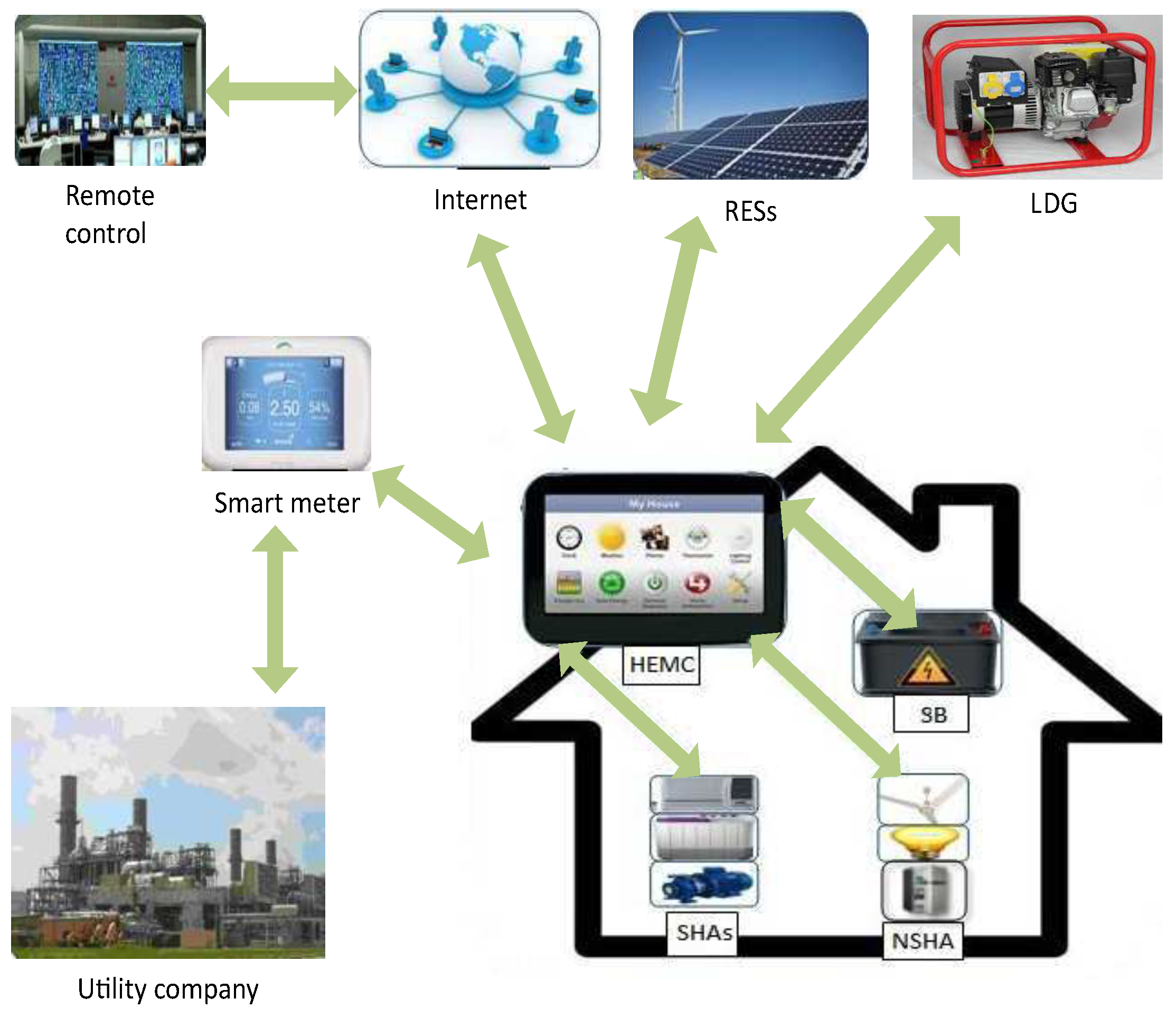
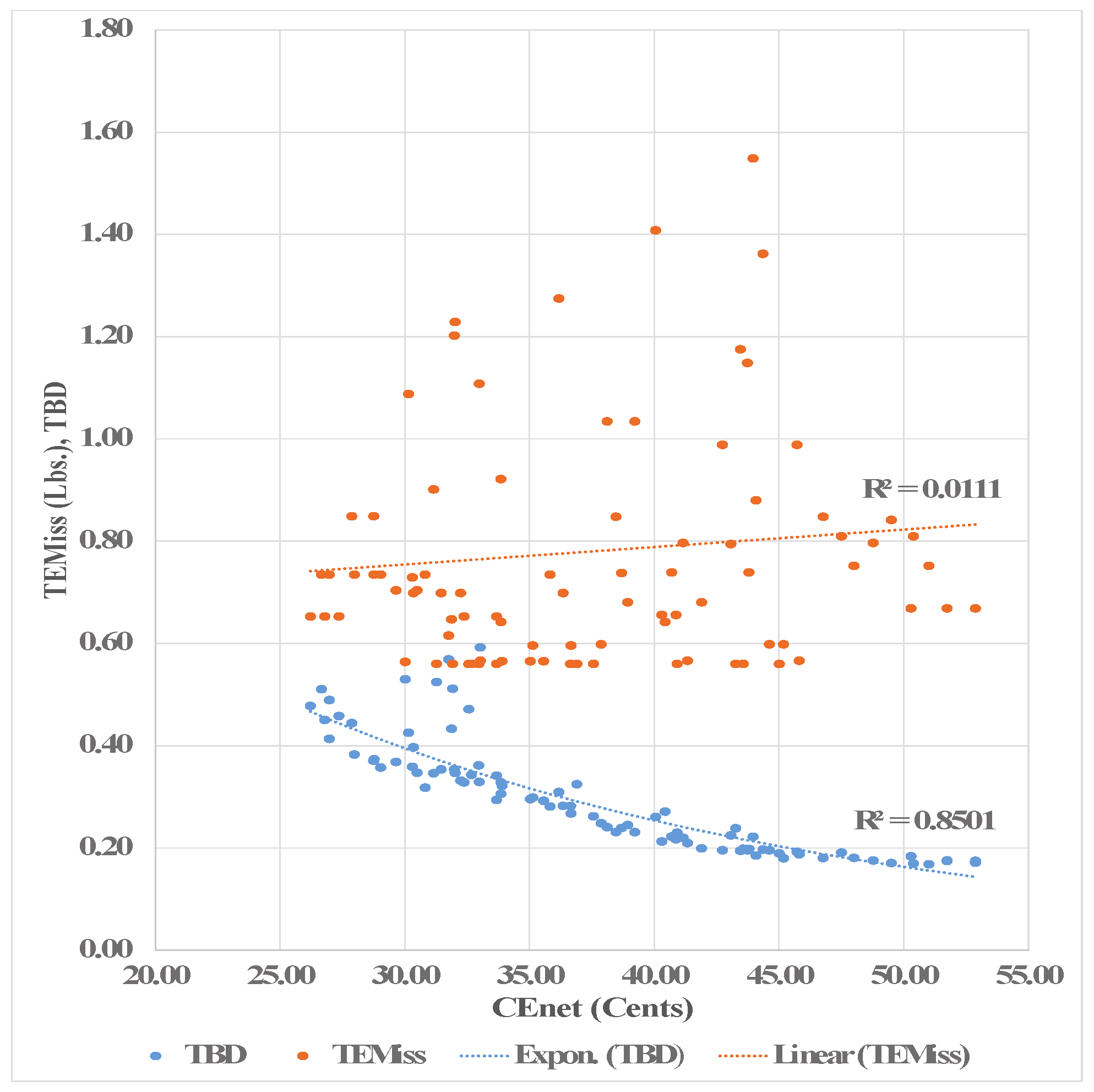
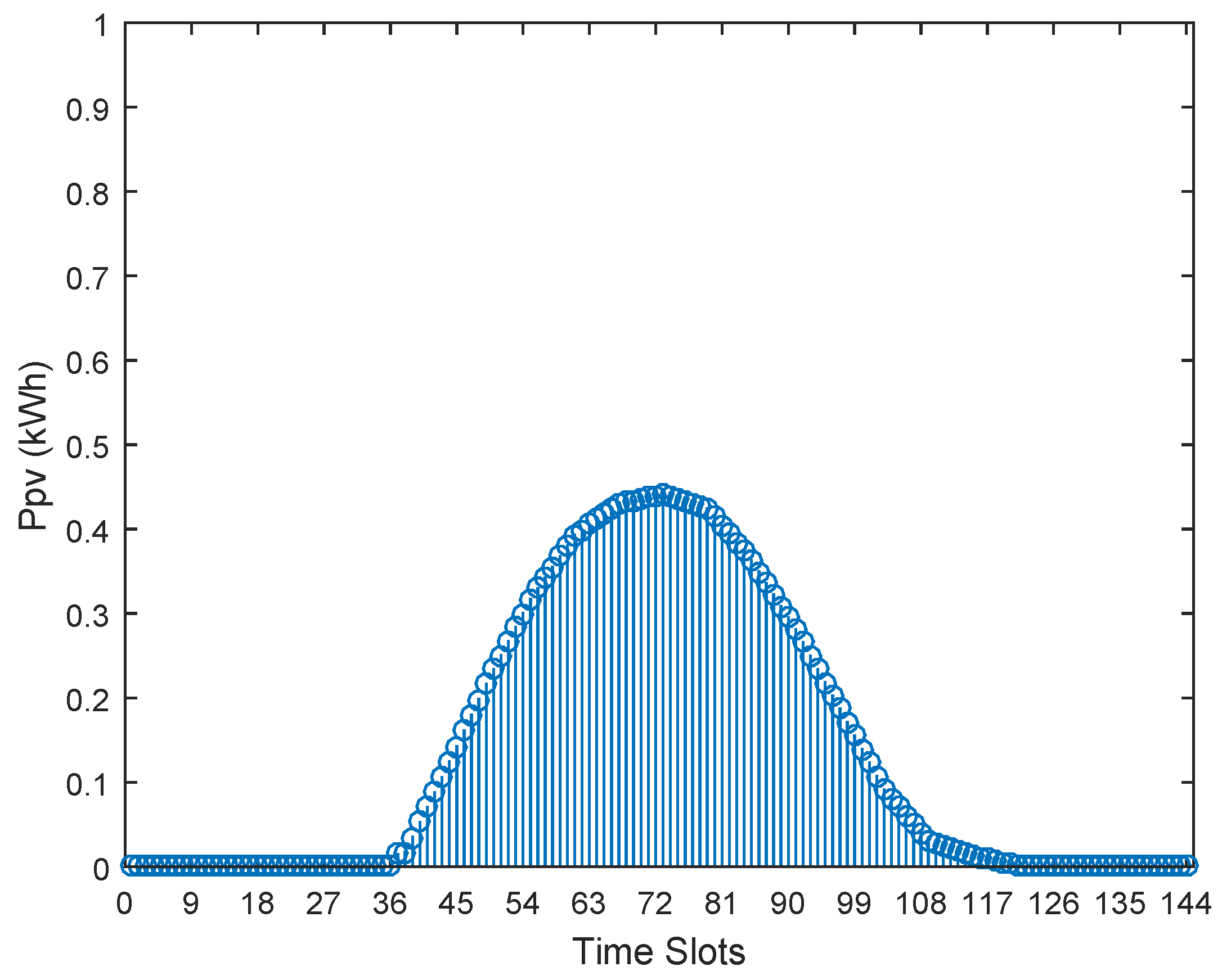
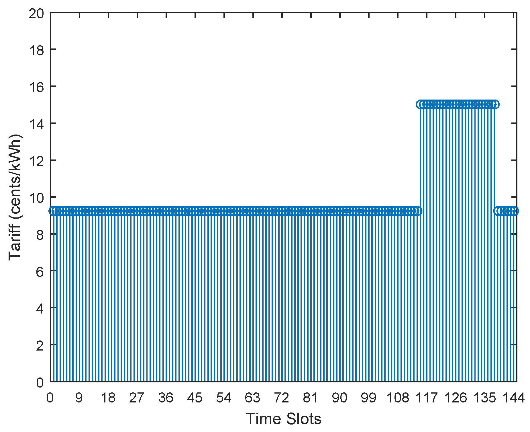
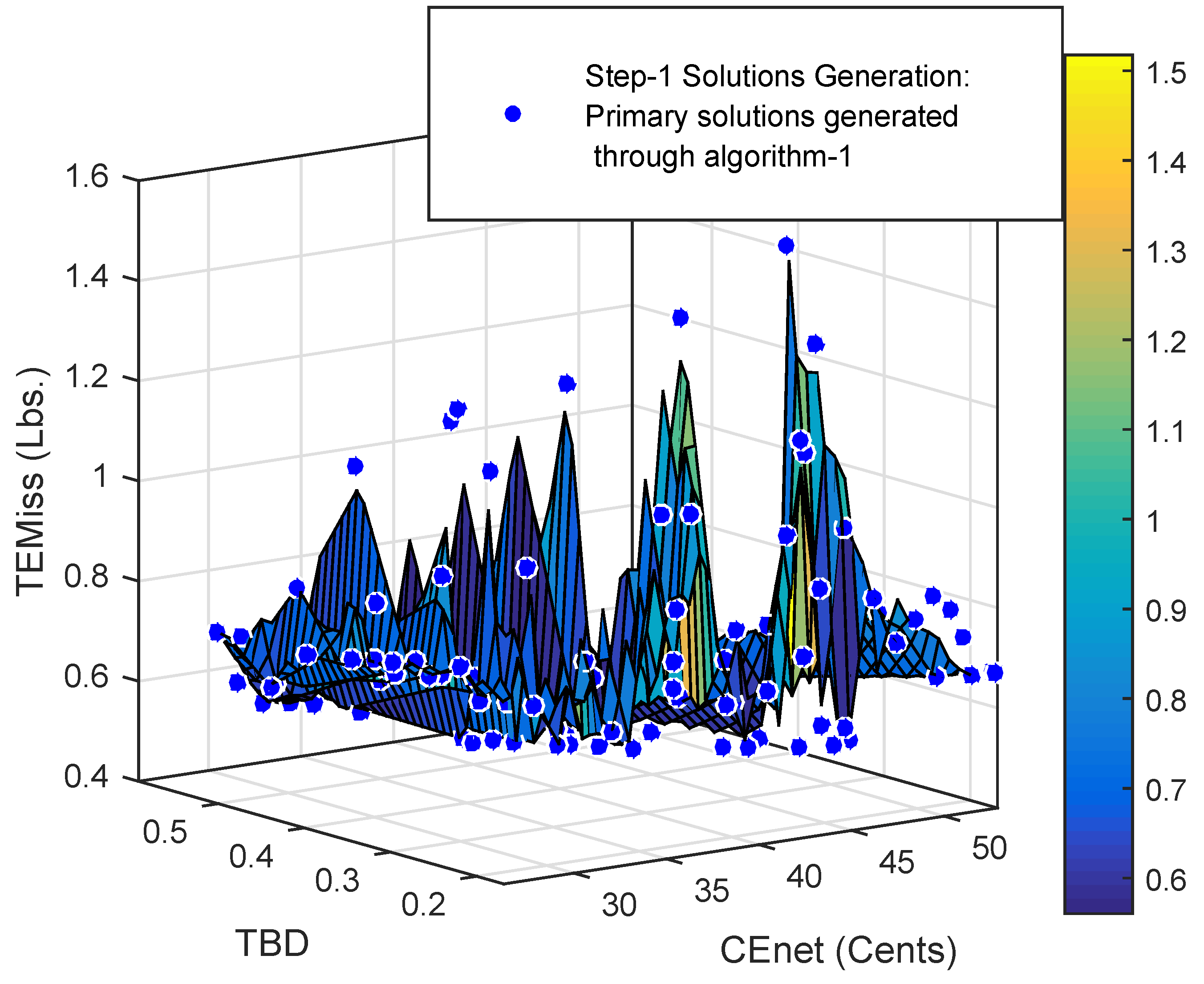
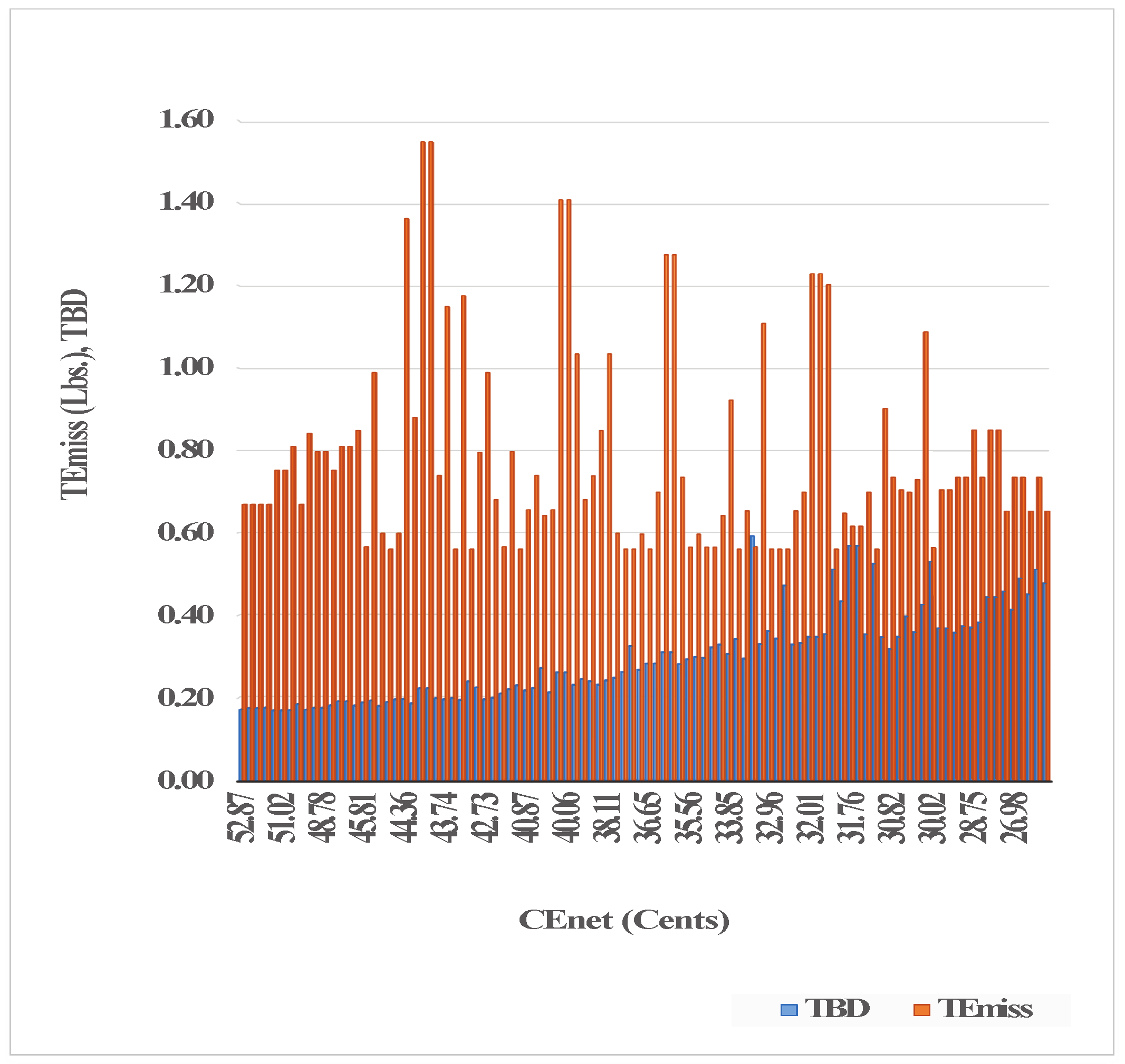
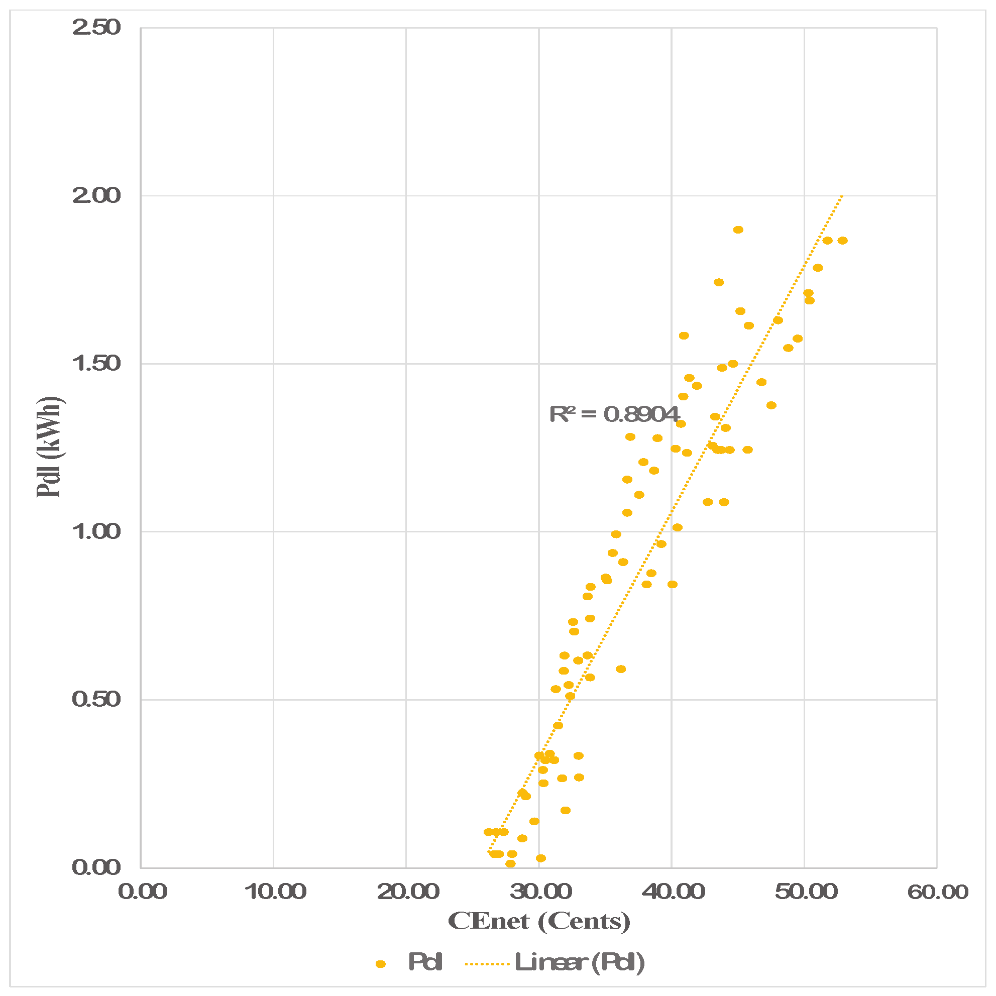
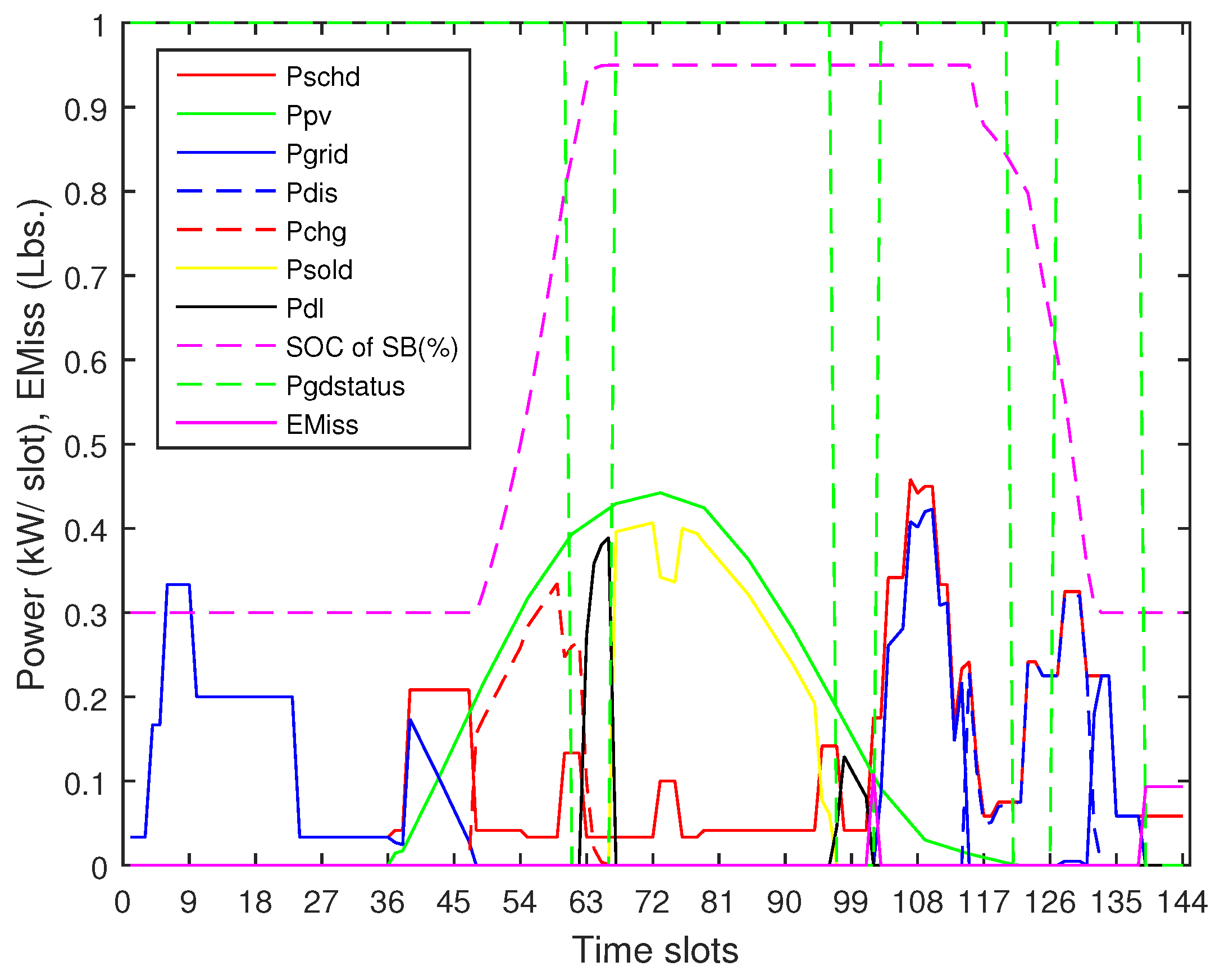
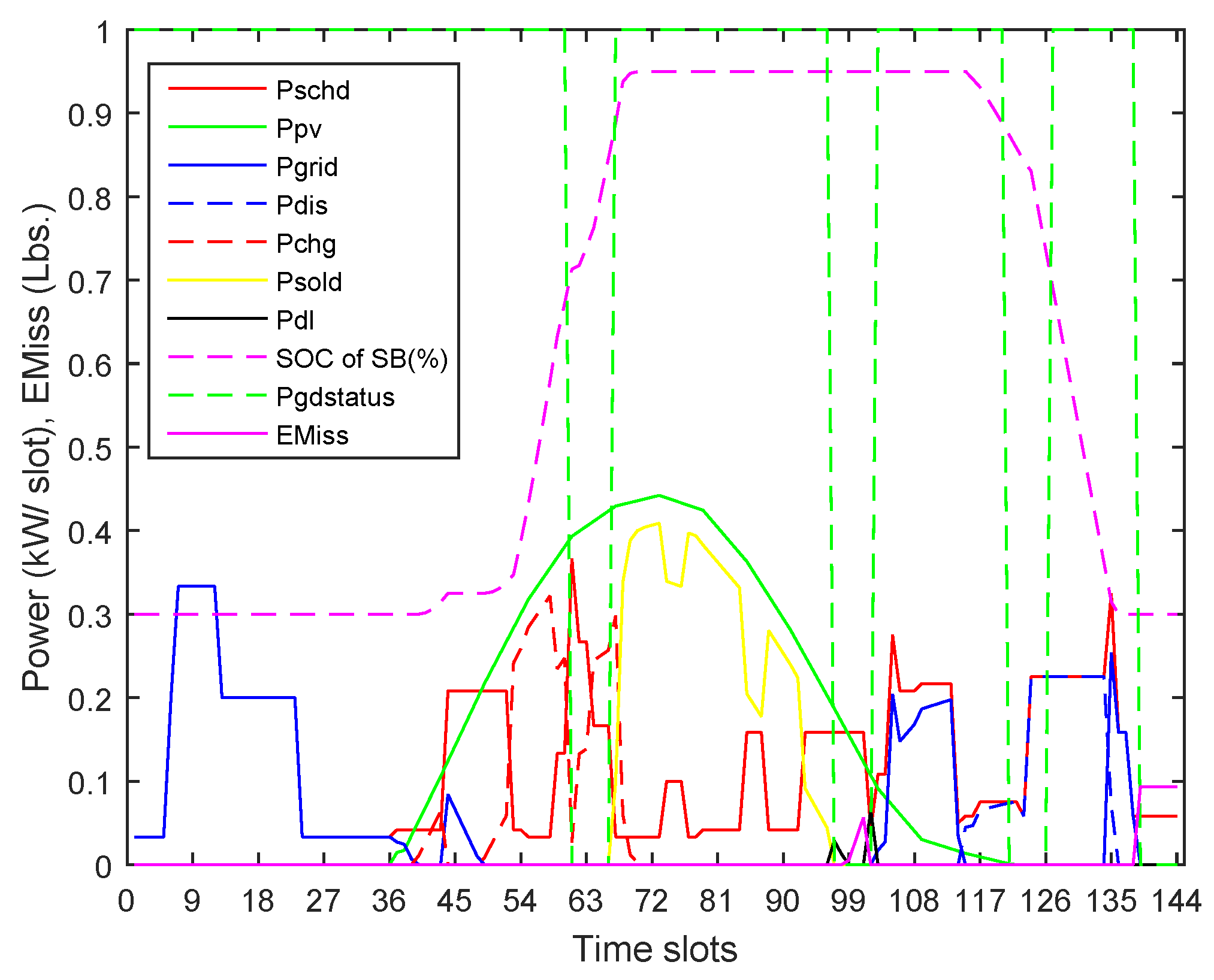

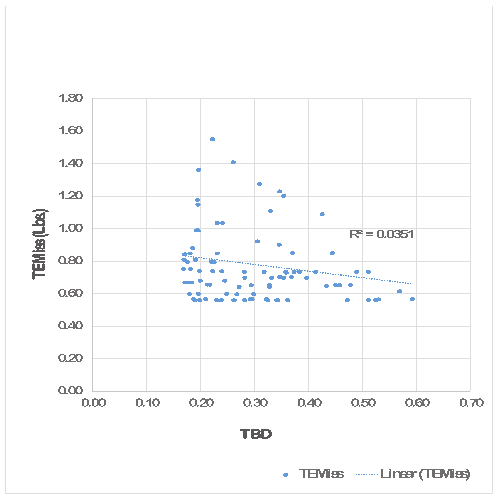
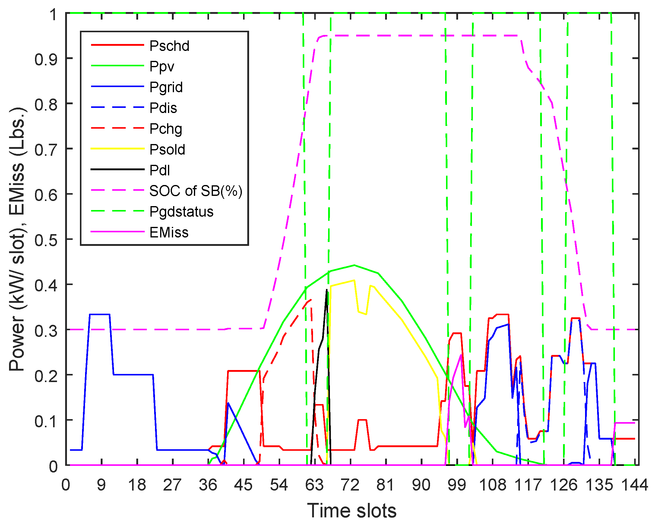

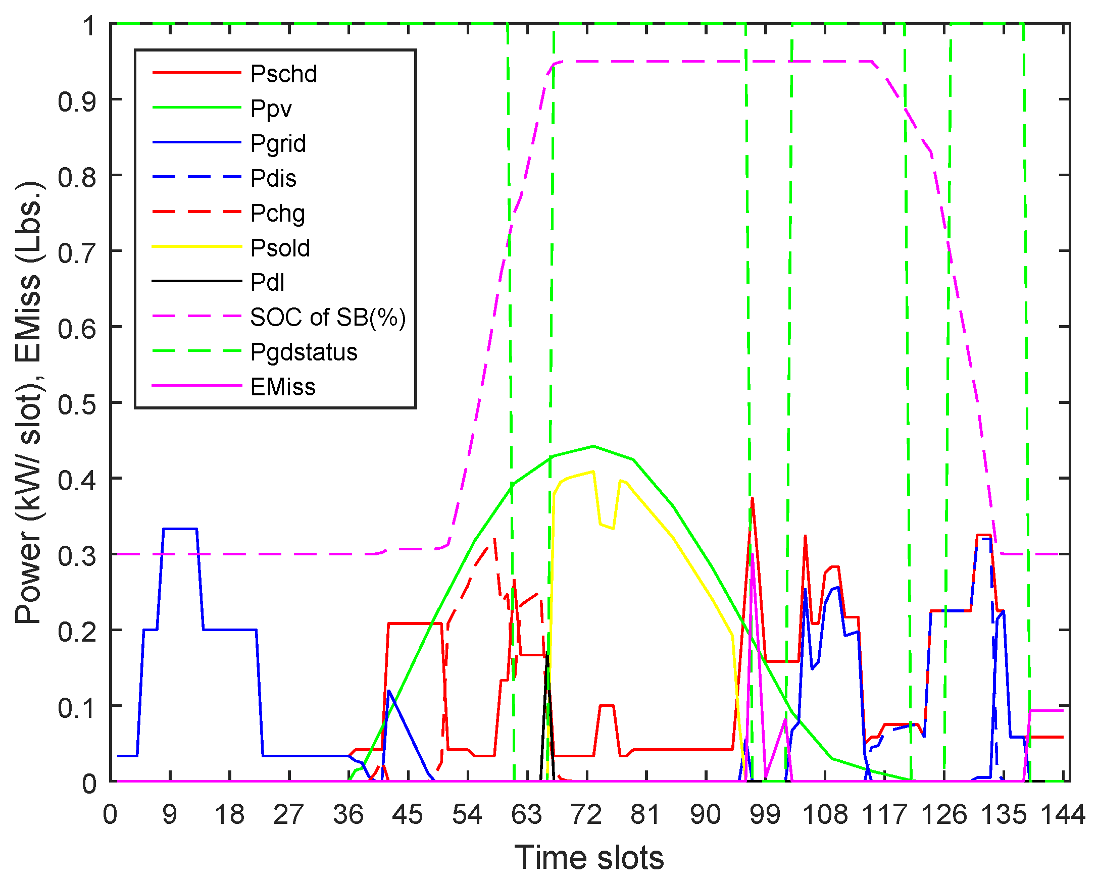

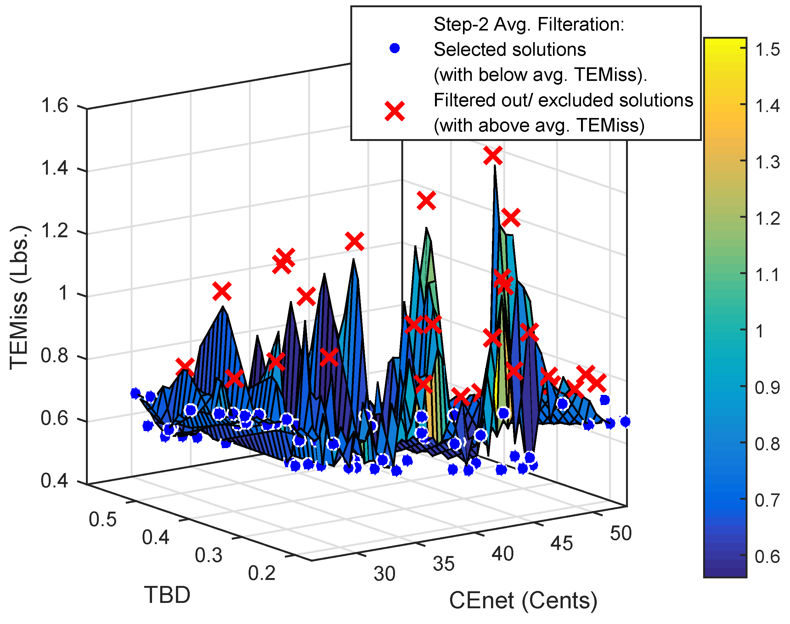
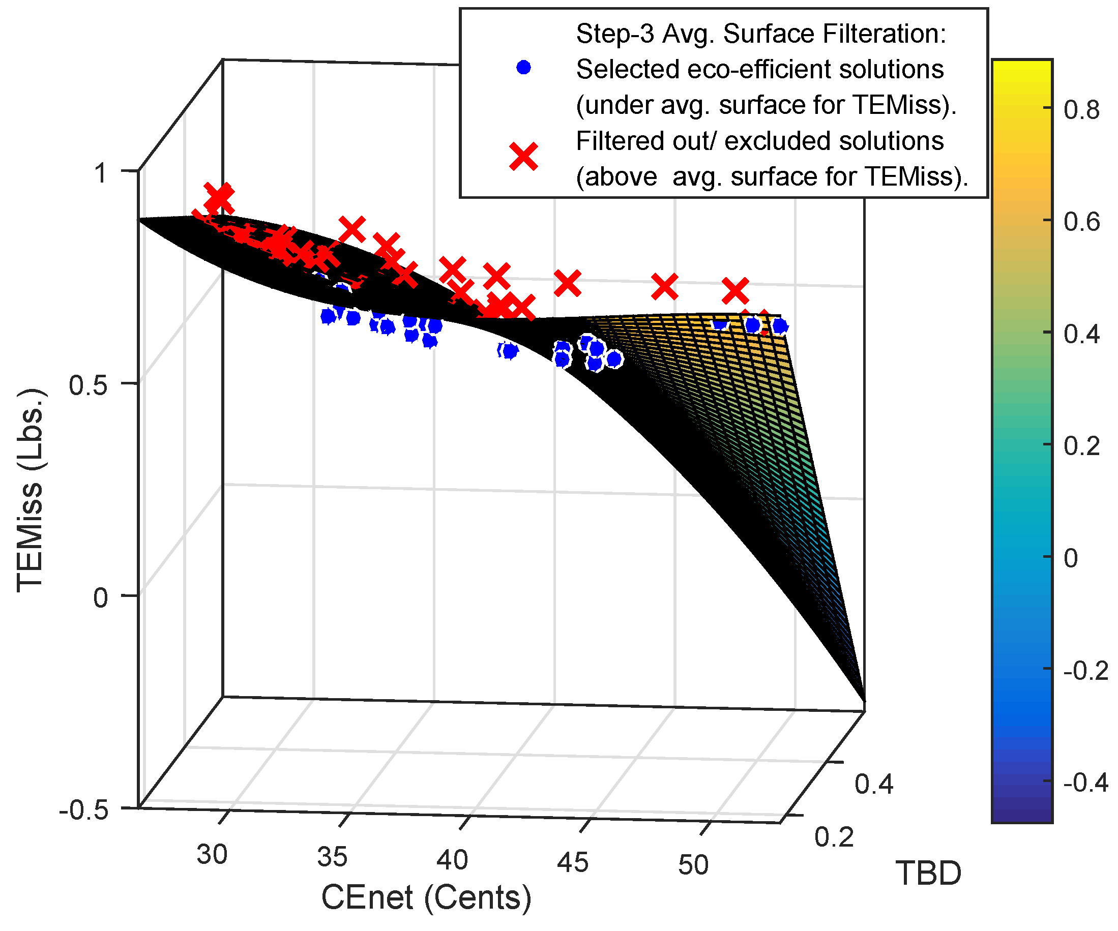
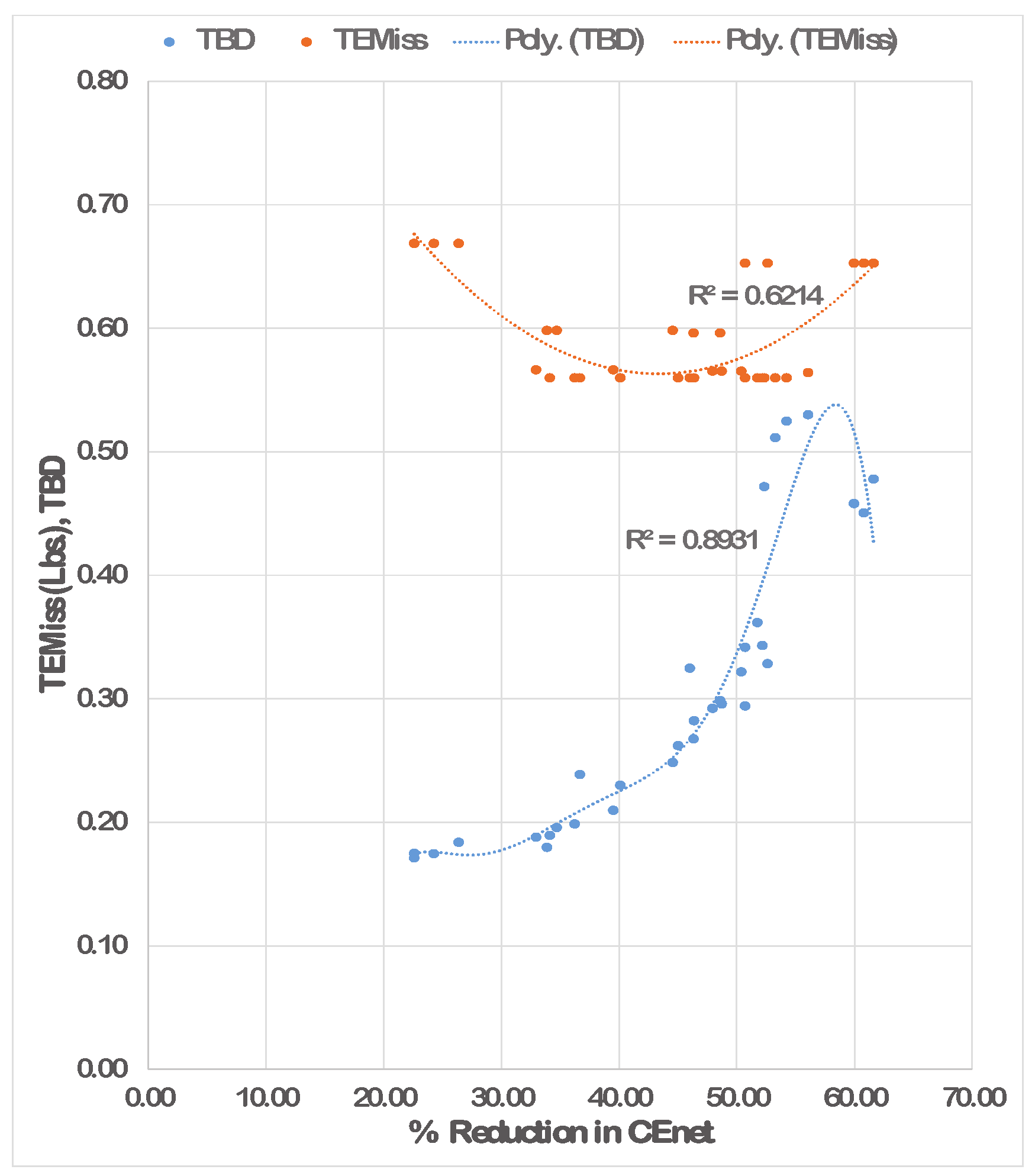
