Optimizing Biodiesel Production from Waste Cooking Oil Using Genetic Algorithm-Based Support Vector Machines

Abstract

The ever increasing fuel demands and the limitations of oil reserves have motivated research of renewable and sustainable energy resources to replace, even partially, fossil fuels, which are having a serious environmental impact on global warming and climate change, excessive greenhouse emissions and deforestation. For this reason, an alternative, renewable and biodegradable combustible like biodiesel is necessary. For this purpose, waste cooking oil is a potential replacement for vegetable oils in the production of biodiesel. Direct transesterification of vegetable oils was undertaken to synthesize the biodiesel. Several variables controlled the process. The alkaline catalyst that is used, typically sodium hydroxide (NaOH) or potassium hydroxide (KOH), increases the solubility and speeds up the reaction. Therefore, the methodology that this study suggests for improving the biodiesel production is based on computing techniques for prediction and optimization of these process dimensions. The method builds and selects a group of regression models that predict several properties of biodiesel samples (viscosity turbidity, density, high heating value and yield) based on various attributes of the transesterification process (dosage of catalyst, molar ratio, mixing speed, mixing time, temperature, humidity and impurities). In order to develop it, a Box-Behnken type of Design of Experiment (DoE) was designed that considered the variables that were previously mentioned. Then, using this DoE, biodiesel production features were decided by conducting lab experiments to complete a dataset with real production properties. Subsequently, using this dataset, a group of regression models—linear regression and support vector machines (using linear kernel, polynomial kernel and radial basic function kernel)—were constructed to predict the studied properties of biodiesel and to obtain a better understanding of the process. Finally, several biodiesel optimization scenarios were reached through the application of genetic algorithms to the regression models obtained with greater precision. In this way, it was possible to identify the best combinations of variables, both independent and dependent. These scenarios were based mainly on a desire to improve the biodiesel yield by obtaining a higher heating value, while decreasing the viscosity, density and turbidity. These conditions were achieved when the dosage of catalyst was approximately 1 wt %.

1. Introduction

With the never ending increase in world fuel demand, biodiesel has emerged in recent decades as one of the main alternatives to petroleum diesel [1]. Biodiesel can be used in conventional diesel engines. Engine performance is comparable to that that provided by petroleum. No changes to fuel handling or the delivery systems are required. Diesel fuel is known as a substitute for, or an additive to, diesel fuel. Nevertheless, it is normally produced from fats and oils of plants and animals [2,3]. In addition, waste cooking oil is a potential sustainable alternative for vegetable oils, as it solves the disposal problem and reduces the cost of raw material [4,5]. A vast quantity of waste cooking oil is generated annually. The methods by which it is disposed of pose a problem, and may result in contamination of water in the environment. Thus, using waste cooking oil to produce biodiesel is an excellent way to use it economically, efficiently, and in an eco-friendly manner [6].

Biodiesel is produced from vegetable oils by direct transesterification. Triglycerides react with short-chain alcohols in the process. An alkaline catalyst, usually sodium hydroxide (NaOH) or potassium hydroxide (KOH) is used in the process to improve the solubility and hasten the reaction. (KOH) [7,8,9]; this increases the solubility and speed of the reaction.

The common method to produce biodiesel is by transesterification. In this method, according to stoichiometry, one mole of triglyceride and three moles of alcohol react in the presence of Sodium Hydroxide (NaOH) to produce a mixture of glycol and fatty acid alkali esters (biodiesel) [10,11] (Figure 1). This transesterification process is influenced by several variables that can be optimized. However, expensive and time-consuming laboratory tests are required to optimize those variables in an experimental fashion. The biodiesel yield is affected by such variables as process temperature, type and dosage of catalyst, agitation time and speed, water content and impurities [12,13,14]. Also, the type and quantity of products that are created during frying affect the biodiesel properties and transesterification reaction. For example, the methyl ester yield is affected by the water that is contained in waste cooking oil; this aids in the saponification reaction [15,16,17]. Pretreating the line prior to transesterification is necessary to remove the undesirable compounds that waste cooking oil contains.

Transesterification of waste cooking oil was involved in the present work. The process used NaOH as a base catalyst. Soft computing and machine learning formed the basis of the optimization process; these are useful in solving problems in engineering and optimization [18,19]. Biodiesel production is influenced by several parameters. Therefore, the determination of the optimum values of these parameters is crucial for biodiesel production performance and scaling up. Mathematical and statistical-based models can provide vital information for the understanding, analysis and prediction of transesterification processes and are required for the optimization of parameters of these processes to improve biodiesel properties. Modelling and optimizing biodiesel production processes will contribute to a greater understanding of the transesterification process features like yield and production rate [20].

A successful optimization study for biodiesel manufacturing process could assist manufacturers in the future development of mass production facilities. Traditionally, modelling and optimizing biodiesel have been carried out using Design of Experiments (DoE) [21] and optimization techniques [22,23,24,25]. These approaches have been used extensively and their concepts and limitations are well known. For example, the factorial DoE has been shown to be unappealing, since it is time consuming, resource demanding and requires intensive work when the numbers of input factors are increased [26].

To date, most of the methods used in studies to optimize biodiesel production process conditions are based on Response Surface Methodology (RSM) and Artificial Neural Networks (ANN). However, regression models that have been based on Support Vector Machines (SVM) have also been implanted in recent years. They have been used for the study of the study biodiesel production process conditions and alcoholysis reactions [27]. Following this approach, some researchers modeled and optimized various factors that affect the transesterification process by using regression models that are based on data mining techniques. For example, the molar ratio, reaction temperature and amount of catalyst in biodiesel production were examined in Moradi, et al. [28] as operational conditions with the biodiesel yield estimated with the use of ANN. Fernandez et al. [29] used Genetic Algorithm (GA) and ANN to optimize biodiesel production process parameters. Both works used experimental data as the basis for modelling and optimizing. Corral et al. [23] employed RSM to optimize the biodiesel from waste cooking oil. Mumtaz et al. [24] used RSM to optimize biodiesel that was produced from rice bran and sunflower oil. RSM was used by Mansourpoor and Shariati [25] to optimize biodiesel from sunflower oil. Yuan et al. [21] examined the production of biodiesel from waste rapeseed oil that had a high level of free fatty acids for use as feedstock for biodiesel production. They optimize with RSM the conditions necessary for maximum conversion to biodiesel. They also sought to understand the importance of factors that are relevant to biodiesel production and their interaction.

In addition, many studies have proposed machine learning model approaches, such as ANN or SVM, as alternative methods to solve complex and ill-defined problems [30]. ANN has become popular due to its usefulness in prediction capability, even with small databases. This methodology could be employed in simulators to control and optimize processes. For example, Moradi et al. [28] used ANN to obtain the optimal combination of inputs or process variables in biodiesel yield. Yuste and Dorado developed an ANN model to simulate biodiesel production by the transesterification of used frying olive oil [18]. In addition to proposing the use of ANN for predicting aspects of biodiesel production, various studies have presented ANN combined with an optimization technique for different optimization purposes. For example, Rajendra et al. [29] used hybrid ANN-GA to optimize biodiesel production. In this case, the input parameters for the ANN to generalize the pretreatment process were catalyst concentration, methanol to oil molar ratio, the initial acid value of vegetable oil and reaction time. The output parameter was the final acid value of biodiesel. Betiku and Taiwo [31] used RSM and ANN to optimize bioethanol production using breadfruit as a potential substrate. Mathematical models were also employed in forecasting the bioethanol yield. More recently, Betiku et al. [2] used ANN, combined with GA and RSM, to model and optimize the process parameters of biodiesel production from the Shea tree (Vitellaria paradoxa).

However, although extensively used, both ANN and GA have deficiencies and other techniques can improve the results. Thus, more advances in the hybridization of prediction and optimization algorithms are still required to optimize the transesterification reaction of biodiesel. In one study, Kusumu et al. [27] investigated the variables that affect the acid-catalyzed transesterification process of Ceiba Pentandra oil, using the SVM approach to optimize five aspects of transesterification (catalyst weight, the molar ratio of methanol to oil, reaction temperature, agitation speed, and reaction time) in order to achieve a high yield, and reduce production costs.

The literature contains numerous studies concerning the production of biodiesel using waste cooking oil. However, there are few studies concerning the use of SVM models to model mathematically transesterification process conditions and subsequent optimization using GA. For this reason, the present work examines the effectiveness of using regression techniques that are based on SVM to find and identify the best combination of transesterification process characteristics when waste cooking is used for various biodiesel production optimization scenarios. In this work, process temperature, mixing time, mixing speed, impurities and humidity of waste cooking oil and dosage of catalyst, were considered to be input features. Density, viscosity, turbidity, high heating value, and yield were considered to be outputs features. (Figure 1).

Based on the dataset obtained from the proposed biodiesel production process, SVM regression techniques were applied with different kernels to model the final biodiesel properties features that were selected. Also, a comparison of ordinary Linear Regression (LR) and the previous nonlinear technique was made to determine the influence on non-linearity. Training of these regression models used the data that were obtained by following the DoE that was proposed and used repeated cross-validation [32,33]. Next, the proposed models were tested to determine their degree of generalization. The additional data that were selected at random complete the range of possibilities.

2. Materials and Methods

2.1. Materials

Waste domestic cooking oils were collected from local restaurants to provide raw material for the production of biodiesel by transesterification using NaOH as the catalyst. The synthesis used the following methanol 98% (GR for analysis, Merck, Darmstadt, Germany) and NaOH (GR for analysis, Merck, Darmstadt, Germany) as reagents.

2.2. Design of Experiments and Design Matrix

A DoE is an experimentation method that is structured and systematized and in which all factors vary simultaneously throughout a set of experimental runs. This enables the determination of the relationship between factors that affect dependent responses of the process. DoE [34] is used to minimize the number of experiments required and to obtain sufficient detail to support a hypothesis. It is generally hypothesized that there are a number of variables that decide the value of responses (outputs) that have a differentiable function. These include independent and controllable variables (inputs or design factors) and uncontrollable variables (noise factors). The method that is proposed for development of the DoE entails constructing a design matrix (factor and levels) and measuring experimentally the responses [35]. The input features in this study, and the experimentally selected optimization factors that were used were the following: the quantity of the NaOH catalyst (C), the methanol/oil molar ratio (M), the temperature of the reaction (T), the humidity (H), the stirring speed (S), time (t), and impurities (I). The outputs that were examined were: turbidity (Turb), yield (η), viscosity (µ), density (ρ), and high heating value (HHV). On the basis of the features that were selected, the DoE (

Table 1. Factors and levels applicable to the Box–Behnken DoE.

Inputs	Notation	Magnitude	Levels
			−1	0	+1
Ratio oil	M		6/1	7.5/1	9/1
Catalyst	C	wt %	1	1.5	2
Time	t	Min	20	30	40
Speed	S	Rpm	500	750	1000
Temp	T	°C	20	30	40
Humidity	H	wt %	0	1.5	3
Impurity	I	wt %	0	1.5	3

) was undertaken with a Box–Behnken design [36]. The latter consists of a fractional, three-level design that requires fewer experiments than a full three-level design. The reduction in the number of experiments saves time and expense. In addition, it lessens the difficultly in preparing the initial samples for each experiment.

The DoE that is defined in Table 1 indicates that a design matrix was generated with 56 experiments and their corresponding factors and levels (

Table 2. Design matrix for transesterification process.

Sample	Inputs
	Molar Ratio	Catalyst (wt %)	Time (min)	Speed (rpm)	Temp (°C)	Humidity (wt %)	Impurity (wt %)
25	6	1	30	500	30	1.5	1.5
29	6	1	30	1000	30	1.5	1.5
27	6	2	30	500	30	1.5	1.5
31	6	2	30	1000	30	1.5	1.5
41	6	1.5	20	750	20	1.5	1.5
45	6	1.5	20	750	40	1.5	1.5
9	6	1.5	30	750	30	0	0
13	6	1.5	30	750	30	0	3
11	6	1.5	30	750	30	3	0
15	6	1.5	30	750	30	3	3
43	6	1.5	40	750	20	1.5	1.5
47	6	1.5	40	750	40	1.5	1.5
26	9	1	30	500	30	1.5	1.5
30	9	1	30	1000	30	1.5	1.5
28	9	2	30	500	30	1.5	1.5
32	9	2	30	1000	30	1.5	1.5
42	9	1.5	20	750	20	1.5	1.5
46	9	1.5	20	750	40	1.5	1.5
10	9	1.5	30	750	30	0	0
14	9	1.5	30	750	30	0	3
12	9	1.5	30	750	30	3	0
16	9	1.5	30	750	30	3	3
44	9	1.5	40	750	20	1.5	1.5
48	9	1.5	40	750	40	1.5	1.5
49	7.5	1	20	750	30	0	1.5
53	7.5	1	20	750	30	3	1.5
17	7.5	1	30	750	20	1.5	0
21	7.5	1	30	750	20	1.5	3
19	7.5	1	30	750	40	1.5	0
23	7.5	1	30	750	40	1.5	3
51	7.5	1	40	750	30	0	1.5
55	7.5	1	40	750	30	3	1.5
50	7.5	2	20	750	30	0	1.5
54	7.5	2	20	750	30	3	1.5
18	7.5	2	30	750	20	1.5	0
22	7.5	2	30	750	20	1.5	3
20	7.5	2	30	750	40	1.5	0
24	7.5	2	30	750	40	1.5	3
52	7.5	2	40	750	30	0	1.5
56	7.5	2	40	750	30	3	1.5
33	7.5	1.5	20	500	30	1.5	0
37	7.5	1.5	20	500	30	1.5	3
35	7.5	1.5	20	1000	30	1.5	0
39	7.5	1.5	20	1000	30	1.5	3
1	7.5	1.5	30	500	20	0	1.5
5	7.5	1.5	30	500	20	3	1.5
3	7.5	1.5	30	500	40	0	1.5
7	7.5	1.5	30	500	40	3	1.5
2	7.5	1.5	30	1000	20	0	1.5
6	7.5	1.5	30	1000	20	3	1.5
4	7.5	1.5	30	1000	40	0	1.5
8	7.5	1.5	30	1000	40	3	1.5
34	7.5	1.5	40	500	30	1.5	0
38	7.5	1.5	40	500	30	1.5	3
36	7.5	1.5	40	1000	30	1.5	0
40	7.5	1.5	40	1000	30	1.5	3

). The variable levels that appear in Table 1 address the intervals that commonly appear in the literature in regards to biodiesel production [37,38,39,40,41].

2.3. Experimental Procedure

To remove insoluble impurities, the waste cooking oils that were collected were filtered. Then, they were heated to 100 °C to remove moisture. Experiments on a laboratory scale setup were conducted. The oil was heated to the necessary temperature by a water bath. A magnetic hot plate stirrer that had a temperature controller was used. A constant stirring speed was maintained during each experiment. Then, NaOH and methanol were added. When the reaction had reached the predetermined time, heating and stirring were ended. The biodiesel that was produced was transferred into glass containers and later analyzed to determine the ρ, µ, Turb, HHV and η.

The biodiesel yield was determined by Equation (1) [42].

$$Yied=\frac{weightofproduct\left(g\right)}{weightofrawoil\left(g\right)}\times 100\%$$

(1)

In addition, the following variables were measured in the final biodiesel product: Turbidity by a 2100Q Turbidimeter (HACH, Loveland, CO, USA) and kinematic viscosity by a Cannon–Fenske viscometers (Cannon Instrument Co., State College, PA, USA) at 40 °C per the standard American Society of Testing Materials (ASTM) D445 method [43]. Density was established by a pycnometer following ASTM D941 [44]. The biodiesel HHV was determined by a PARR 1351 bomb calorimeter following the ASTM D240 standard method [45].

2.4. Support Vector Machines

SVM is one of the numerous nonlinear regression techniques. Studied intensively, it is applied for its use as a universal approximation [46,47,48]. A kernel-based algorithm is the basis of this method. SVM has sparse solutions. Its predictions for new inputs depend on the kernel function evaluation at a subcategory of occurrences during a training stage. The objective of this method is to find a function to minimize the final error in Equation (2).

$$y\left(x\right)=w^T·\varphi \left(x\right)+b$$

(2)

where y(x) is the predicted value, w is the vector with parameters that define the model, b is the value of the bias and ϕ(x) fixes the feature-space transformation. In this method, the error function that appears in the simple linear regression (Equation (3)) is replaced by an $ϵ$ insensitive error function (Equation (4)). The latter assigns a zero to values when $ϵ$ exceeds the difference between the target and the predicted value. If the difference is not less than $ϵ$, the error function maintains its value. (The foregoing appears to be a contradiction.) In order to minimize Equation (5), a cost (C) is also assigned to the difference between the target and predicted values.

$$\frac{1}{2}{\displaystyle {\displaystyle \sum }_{n=1}^N}{\left[y_n-t_n\right]}^2+\frac{\lambda }{2}{\Vert w\Vert }^2$$

(3)

$$E_{ϵ}\left(y\left(x\right)-t\right)=\{\begin{array}{cc}0,& if \left|y\left(x\right)-t\right|<ϵ\\ \left|y\left(x\right)-t\right|-ϵ,& otherwise\end{array}$$

(4)

$$C{\displaystyle {\displaystyle \sum }_{n=1}^N}{E}_{ϵ}\left(y\left(x_n\right)-t_n\right)+\frac{1}{2}{\Vert w\Vert }^2$$

(5)

where y(x) is the value that Equation (2) predicts, t is the searched target function, ϵ is the margin where the function does not penalize, and C is the penalty. The process is optimized, but the initial function (Equation (2)) increases in complexity (Equation (6)).

$$y\left(x\right)={\displaystyle {\displaystyle \sum }_{n=1}^N}\left({\alpha }_i-{\alpha }_i{}^{\ast }\right)\langle x_i·x\rangle +b$$

(6)

where α is one solution for the optimization problem that Lagrangian Theory makes possible. The data is transformed by the function to a higher dimensional feature space. This increases the accuracy of the nonlinear problem. Thus, the final function resembles Equation (7).

$$y\left(x\right)={\displaystyle {\displaystyle \sum }_{n=1}^N}\left({\alpha }_i-{\alpha }_i{}^{\ast }\right)k\left(x_i, x\right)+b$$

(7)

This case uses functions of three kernels. They are linear (Equation (8)), polynomial (Equation (9)) and Gaussian Radial Basis Function (RBF) (Equation (10)).

$$k\left(x_i, x\right)=x_i{}^{T}x$$

(8)

$$k\left(x_i, x\right)=\langle x_i·x\rangle {}^d$$

(9)

$$k\left(x_i, x\right)=e^{-\frac{\Vert x_i-x\Vert {}^2}{2{\sigma }^2}}$$

(10)

To program the methodology that was proposed, generate the design matrix and develop the regression models, R statistical software was selected [20].

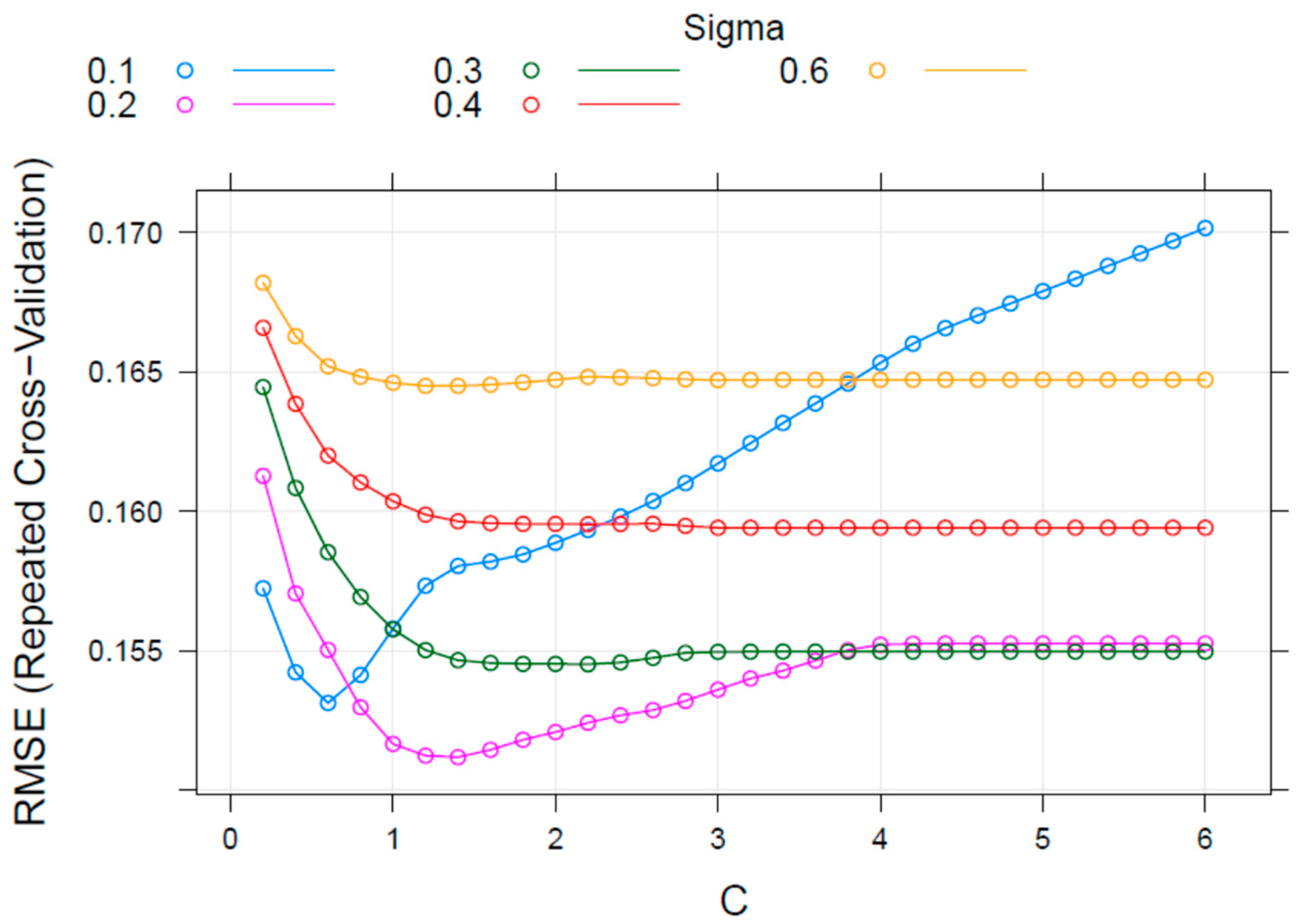
To undertake this part of the method, the SVM models were trained by using 50 times repeated 10fold cross-validation. Their calculation times were not long. This made possible the use of the entire training dataset that came from the DoE, and was formed by 56 entries to create the models. However, it was necessary to first divide the initial database into 10 subsets, using nine subsets to build the model and using the tenth subset to calculate the error. Other errors were obtained when the procedure was repeated an additional 50 times. Finally, the arithmetic mean of all errors of the process was calculated. In addition, the various algorithms were trained, significant parameters for each algorithm were tuned, and their values that produced the best predictive performance were identified. The accuracy of the predictions were judged by means of the Root Mean Square Error (RMSE) and the correlation of real and predicted values.

Finally, after the most accurate models were built, selected and trained, they were tested in the laboratory in nine experiments and with new samples, to determine their real degree of generalization.

3. Genetic Algorithms for Optimization of Biodiesel Production Features

Regression models that had the best generalization capacity were selected to identify the best combinations of transesterification attributes that would yield desirable biodiesel production properties. The intention was to study and optimize nine different scenarios in biodiesel production from waste cooking oil. These were: maximizing η, minimizing Turb, minimizing ρ and µ, maximizing the HHV, minimizing C, minimizing S, minimizing t and minimizing M. The search for the best combination used GA-based evolutionary optimization techniques. Using these techniques for the optimization of industrial processes and devices [49,50,51,52,53,54] has been proven previously in the literature. GA conducts optimization with a population of several individuals in a way that resembles the behavior of biological process. The resulting solution approximates in general the global minimum of all possibilities [55]. The optimization using GA involves the six following steps, (see Figure 2), [56,57].

(1)

Coding/decoding: The information from feature values for each individual is changed to binary codes that join to form chromosomes, and vice versa. Values that are out of the range proposed by DoE is replaced.

(2)

Population initialization: The initial population is generated by a random set of individuals.

(3)

Evaluation: The responses of models are evaluated by a fitness function to determinate the individuals that will be part of the next generation.

(4)

Selection: Sorting of individuals uses the criterion that the fitness function provides. The top 25% of individuals are selected for the next generation.

(5)

Crossover: Portions of two parents of the current generation have been combined to form a new offspring. These portions have been selected on the basis of two positions and two longitudes. The majority (60%) of the new population consists of new offspring who were created by crossovers from selected parents and h the crossovers consisting of a change in a random number of bits of chromosomes of, alternatively, two randomly selected best individuals.

(6)

Mutation: Several individuals were selected from the 25% who had been chosen and the 60% who had been, were created by crossovers. This was done on the basis of a uniform probability and a random element of the chromosome that was flipped to create a new individual. Mutation is responsible for 15% of the new population.

The optimization process that provides in each scenario the best combination of transesterification attributes was the following: First, 1000 individuals transesterification parameters (M, C, T, S, t, H, I) or combinations thereof were randomly generated corresponding to the range that appears in Table 1. These first individuals or combinations formed the initial generation, generation 0. Based on these individuals, the variables that define biodiesel properties were predicted by the regression models that had the best generalization capacity in each case (SVM or LR models). Based on this prediction, an error obtained from a defined fitness function (J₁) permitted the selection of the individuals for the subsequent generations. In this case, the fitness function that was developed considered the maximization or minimization of the studied features, and the weights of the different proposed scenarios (Equation (11)).

$$\begin{gathered} J_1={\omega }_1·P_{\eta }{}^{max}+{\omega }_2·P_{HHV}{}^{max}+{\omega }_3·P_{Turb}{}^{min}+{\omega }_4·P_{\rho }{}^{min}+{\omega }_5·P_{\mu }{}^{min}+ \\ {\omega }_6·P_M{}^{min}+{\omega }_7·P_C{}^{min}+{\omega }_8·P_S{}^{min}+{\omega }_9·P_t{}^{min} \end{gathered}$$

(11)

where ${\omega }_i$ are the weights that are applied to each component in the fitness function J₁, and $P_j{}^{max,min}$ defines the objective sought for each of the features.

These weights ${\omega }_i$ were so defined that the above-mentioned optimization scenarios would be achieved.

Table 3. Different proposed scenarios with weights of each component of the fitness function.

Scenario	${\mathit{\omega }}_1$	${\mathit{\omega }}_2$	${\mathit{\omega }}_3$	${\mathit{\omega }}_4$	${\mathit{\omega }}_5$	${\mathit{\omega }}_6$	${\mathit{\omega }}_7$	${\mathit{\omega }}_8$	${\mathit{\omega }}_9$
1	1	1	1	1	1	0	0	0	0
2	1	0.3	0.3	0.3	0.3	0	0	0	0
3	0.3	1	0.3	0.3	0.3	0	0	0	0
4	0.3	0.3	1	0.3	0.3	0	0	0	0
5	0.3	0.3	0.3	1	1	0	0	0	0
6	1	1	1	1	1	0	1	0	0
7	1	1	1	1	1	0	0	1	0
8	1	1	1	1	1	0	0	0	1
9	1	1	1	1	1	1	0	0	0

shows the weights ${\omega }_i$ of each variable that are part of the fitness function J₁ to optimize the biodiesel production process for the nine different optimization scenarios.

After selecting 25% of the best individuals (i.e., 250) according to the fitness function (J₁) and the optimization scenarios that were selected, the crossover process was undertaken. It was first necessary for two selected parents to provide two complete chromosomes. Each chromosome was then coded in binary code. Then, a random number of crossings (1, 2, 3, or 4) was selected. Also, a number was randomly selected for each crossing to define for each crossing the initial bit’s position. The longitude of the number of bits in the chromosome’s crossing part was selected similarly. This information was used in selecting some of the first parent’s bits. The second parent donated the remaining bits to create a new chromosome and generation. Positions 1 and 2 appear in Figure 2. Figure 2 also shows the lengths (longitude 1) and (longitude 2) that were used to cross two individuals from generation “0”. Positions 1 and 2 were equal to “10” and “47” respectively. Longitudes 1 and 2 were equal to “9” and “10” respectively. (Values of all positions and longitudes are in bits). Finally, the binary code of new chromosomes was decoded in order to generate new individuals. The latter were formed by parameters that required adjustment to complete 60% of the new population (i.e., generation 1), namely 600 individuals. The remaining individuals (i.e., 15% or 150 individuals) were generated randomly to complete the new generation (i.e., generation 0).

4. Results

4.1 Experimental Results

Table 4. Experimental results based on the Box–Behnken DoE.

Sample	Outputs
	η	Turb (NTU)	ρ (g/mL)	µ (mm2/s)	HHV (MJ/kg)
25	93	0.65	0.83	7.03	42.70
29	93	1.05	0.85	5.15	41.83
27	40	1.78	0.822	5.65	42.06
31	9.5	58.5	0.83	5.05	41.78
41	29	8.48	0.84	5.40	41.94
45	29	0.21	0.85	5.93	42.19
9	87	86	0.83	6.00	42.22
13	76	1	0.86	5.40	41.94
11	75	1.89	0.85	8.05	43.17
15	77	1.18	0.83	5.39	41.94
43	31	2.44	0.85	4.67	41.61
47	57	2.94	0.79	7.40	42.87
26	88	6	0.83	9.83	43.99
30	55	3.52	0.80	6.07	42.26
28	50	3.81	0.79	9.24	43.72
32	23	1.66	0.79	6.38	42.40
42	59	1.09	0.81	6.16	42.30
46	91	2.45	0.83	7.97	43.13
10	83	6.29	0.82	5.67	42.07
14	90	1.42	0.80	5.65	42.06
12	90	1.01	0.82	7.81	43.06
16	71	10.14	0.85	10.15	44.14
44	85	0.67	0.84	6.15	42.29
48	82	1.01	0.81	6.17	42.30
49	93	1.47	0.80	8.96	43.59
53	89	1.62	0.82	8.20	43.24
17	92	1.06	0.81	6.47	42.44
21	95	0.69	0.82	9.40	43.79
19	91	1.53	0.83	9.43	43.81
23	86	1.61	0.81	7.24	42.80
51	94	0.22	0.84	6.13	42.28
55	89	0.42	0.83	11.99	44.99
50	63	0.34	0.82	0	39.45
54	87	0.36	0.81	4.48	41.52
18	45.5	53	0.82	5.97	42.21
22	23	1.09	0.82	5.32	41.91
20	24.6	0.64	0.80	6.07	42.25
24	22	18.03	0.81	4.67	41.61
52	66	0.31	0.81	4.08	41.33
56	90	1.01	0.84	5.77	42.12
33	93	1.18	0.82	5.65	42.06
37	83	1.34	0.84	8.22	43.25
35	100	0.56	0.81	6.10	42.27
39	93	0.72	0.73	6.36	42.39
1	98	0.48	0.84	3.78	41.20
5	75	1.85	0.79	11.98	44.99
3	86	2	0.81	4.82	41.68
7	86	1.59	0.77	7.15	42.75
2	83	2.71	0.79	12.14	45.06
6	82	0.9	0.82	8.16	43.22
4	88	0.63	0.83	6.03	42.23
8	95	0.94	0.81	6.35	42.38
34	78	0.74	0.81	5.83	42.14
38	77	7.42	0.82	8.59	43.42
36	93	0.78	0.83	5.54	42.01
40	85	1.96	0.82	7.81	43.06

shows the results obtained experimentally for the attributes of the transesterification process (ρ, µ, Turb, HHV, η) according to the Box–Behnken DoE design matrix (Table 2).

4.2. Analysis of the Uncertainty

The analysis of variance (ANOVA) was examined to evaluate the uncertainty in the experimental measurements due to the proposed DoE. The five properties of the biodiesel that were studied experimentally were compared to the seven transesterification process attributes to identify any relationships (

Table 5. Results of the analysis of the variance of the five output features.

	η		Turb		ρ		µ		HHV
	p-Value		p-Value		p-Value		p-Value		p-Value
Molar Ratio	0.09459	.	0.08468	.	0.03046	*	0.07618	.	0.07549	.
Catalyst	4.91 × 10−6	***	0.10095		0.31188		0.00050	***	0.00049	***
Time	0.85788		0.99890		0.31188		0.45523		0.45600
Speed	0.63687		0.53505		0.57979		0.45992		0.45890
Temp	0.69014		0.57371		0.35746		0.47761		0.47506
Humidity	0.99206		0.27337		0.92636		0.00411	**	0.00406	**
Impurity	0.46221		0.14076		0.71178		0.53145		0.53015

Significant codes according to p-value: ‘***’ 0.001, ‘**’ 0.01, ‘*’ 0.05, ‘.’ 0.1.

).

The p-values that were obtained had low values for two features, C and M. This indicates that the apparent relationships were statistically significant. Therefore, a p-value of less than 0.1 was considered to denote low uncertainty. Consequently, the model had no predictive usefulness and could be rejected. In this case, C satisfies this condition for each of µ, HHV, and η.

4.3. Regresion Models Based on Data Mining Tecniques

After selecting the features of the final data set, the next steps were to train, test and validate prediction models. The construction of regression models that predict aspects of a biodiesel production process borrowed from machine learning techniques that use SVM technique. In addition, LR was used to be able to compare linear and nonlinear techniques. The method in this case was to conduct 56 experiments according to the proposed DoE. The resulting data were normalized to between 0 and 1. The models were trained by using these 56 instances by 50 times repeated 10fold cross-validation. The RMSE and the real and predicted values correlation were obtained during training to permit the models’ accuracy to be compared. Meanwhile, each algorithm’s most important parameters were tuned to improve the prediction capabilities. For example, Figure 3 gives the RMSE for output feature ‘µ’ that is training an SVM that has an RBF kernel when parameters, such as cost and σ vary. The most accurate model in this case had a cost equal to 1.4 and an σ equal to 0.2.

Nine new experiments were conducted for the purpose of testing the models with data that had not been used previously during training (

Table 6. Test matrix for transesterification process.

Sample	Inputs
	Molar Ratio	Catalyst (wt %)	Time (min)	Speed (rpm)	T (°C)	Humidity (wt %)	Impurity (wt %)
t-1	8.33	1.3	20	990	36.5	2.17	0.55
t-2	8.77	1.5	40	805	26	2.07	1.84
t-3	8.4	1.3	21	912	36	2.3	0.17
t-4	8.34	1.2	22	1000	32	0.4	3
t-5	7.67	1	24	840	32	0	1.12
t-6	7.88	1.2	20	989	34.2	0.95	0.2
t-7	8.13	1	27	717	30	0	3
t-8	8.43	1.38	20	1000	37.5	2.67	0.78
t-9	6	1	27	500	29	0	0

and

Table 7. Results of the experiments performed in the testing stage.

Sample	Outputs
	η	Turb (NTU)	ρ (g/mL)	µ (mm2/s)	HHV (MJ/kg)
t-1	78	0.28	0.77	4.34	41.46
t-2	79	0.27	0.77	4.69	41.62
t-3	20	31.8	0.75	4.93	41.73
t-4	67	0.17	0.79	4.79	41.66
t-5	38	0.59	0.73	4.78	41.66
t-6	32	0.14	0.78	4.66	41.61
t-7	69	0.63	0.76	7.02	42.7
t-8	55	0.15	0.74	4.83	41.69
t-9	84	1.75	0.78	6.09	42.27

). These new data were selected randomly and sought to cover all possibilities of the problem from previous DoE and, also, to avoid overtraining the models. The training and testing stages’ results appear in

Table 8. Results obtained during the training and testing stages for η.

η
	Training (Cross Validation)		Testing
	RMSE (%)	Correlation	RMSE (%)	Correlation
SVM (Linear kernel)	23.64	34.56	25.76	71.94
SVM (Polinomial kernel)	23.59	34.56	25.83	71.79
SVM (RBF kernel)	22.71	83.03	25.41	51.53
LR	23.49	38.73	21.38	69.56

,

Table 9. Results obtained during training and testing stage for Turb.

Turb
	Training (Cross Validation)		Testing
	RMSE (%)	Correlation	RMSE (%)	Correlation
SVM (Linear kernel)	11.56	1.71	10.43	56.96
SVM (Polinomial kernel)	11.64	1.64	10.43	57.15
SVM (RBF kernel)	11.56	35.53	10.58	0.01
LR	15.75	17.35	12.72	0.01

,

Table 10. Results obtained during the training and testing stages for ρ.

ρ
	Training (Cross Validation)		Testing
	RMSE (%)	Correlation	RMSE (%)	Correlation
SVM (Linear kernel)	15.61	13.73	45.45	2.62
SVM (Polinomial kernel)	15.64	13.02	44.91	4.77
SVM (RBF kernel)	15.50	36.10	44.91	4.77
LR	16.81	14.86	44.57	0.91

,

Table 11. Results obtained during the training and testing stages for µ.

µ
	Training (Cross Validation)		Testing
	RMSE (%)	Correlation	RMSE (%)	Correlation
SVM (Linear kernel)	15.14	31.01	14.72	7.69
SVM (Polinomial kernel)	14.07	33.43	15.49	5.82
SVM (RBF kernel)	15.18	86.05	16.64	18.35
LR	14.96	37.11	18.47	9.44

and

Table 12. Results obtained during the training and testing stages for HHV.

HHV
	Training (Cross Validation)		Testing
	RMSE (%)	Correlation	RMSE (%)	Correlation
SVM (Linear kernel)	15.22	31.06	14.67	7.31
SVM (Polinomial kernel)	14.03	33.30	15.44	5.35
SVM (RBF kernel)	15.13	88.55	16.96	17.90
LR	14.88	37.17	18.44	9.18

(selected models are in are in bold letters).

A lower RMSE in training and testing usually implied a higher correlation. As a result, these conditions determined the model selection process. Nevertheless, the experts in some cases selected a model based on results obtained, although also considering other criteria. For example, in the case of HHV and µ, the models that were selected did not have fewer errors. However, some had outliers (Figure 4) that, when removed, improved the predictions of the selected models. This caused their selection.

4.4. Optimization of Biodiesel Production Process Based on Genetic Algorithms

Once the models were selected on the basis of their accuracy and relevance to the problem, GA was applied to optimize the process. In this case, the regression models that had the best generalization capacity (SVM with polynomial kernel for Turb and SVM with RBF kernel for η, ρ, µ and HHV) were used to search for the values of the features that define biodiesel production in the hope of finding some fixed biodiesel properties.

Results of this search are shown in

Table 13. Optimization scenarios: Comparison of feature combination for the optimization of the biodiesel process. Pre: predicted values; Real: experimental values.

	Optimization Scenarios
	1st Scenario		2nd Scenario		3rd Scenario		4th Scenario		5th Scenario		6th Scenario		7th Scenario		8th Scenario		9th Scenario
	Pre	Real	Pre	Real	Pre	Real	Pre	Real	Pre	Real	Pre	Real	Pre	Real	Pre	Real	Pre	Real
Molar ratio	8.33	8.33	8.40	8.40	7.88	7.88	8.34	8.34	7.67	7.67	8.13	8.13	8.32	8.32	8.43	8.43	6.00	6.00
Catalyst (wt %)	1.31	1.31	1.27	1.27	1.18	1.18	1.21	1.21	1.06	1.06	1.00	1.00	1.09	1.09	1.38	1.38	1.00	1.00
Time (min)	20.02	20.02	20.86	20.86	20.00	20.00	22.03	22.03	24.04	24.04	26.94	26.94	26.80	26.80	20.00	20.00	26.79	26.79
Speed (rpm)	991.90	991.90	911.53	911.53	988.98	988.98	999.99	999.99	840.00	840.00	716.99	716.99	500.00	500.00	998.98	998.98	500.00	500.00
T (°C)	36.30	36.30	35.96	35.96	34.22	34.22	31.99	31.99	31.72	31.72	30.04	30.04	33.47	33.47	37.60	37.60	28.75	28.75
Humidity (wt %)	2.16	2.16	2.31	2.31	0.95	0.95	0.41	0.41	0.00	0.00	0.00	0.00	0.003	0.003	2.69	2.69	0.00	0.00
Impurity (wt %)	0.54	0.54	0.17	0.17	0.19	0.19	2.99	2.99	1.11	1.11	2.93	2.93	2.22	2.22	0.78	0.78	0.00	0.00
η	100	94.00	100	96.00	100	92.00	94.66	93.00	98.30	93.00	99.99	87.00	100	93.00	99.99	91.00	98.77	87.00
Turb	2.15	1.76	2.18	1.97	1.90	1.78	1.98	1.87	1.80	1.93	1.95	1.97	2.01	1.89	2.26	2.37	1.81	1.78
ρ	0.81	0.79	0.81	0.76	0.81	0.83	0.81	0.81	0.82	0.82	0.81	0.76	0.81	0.84	0.81	0.81	0.82	0.83
µ	6.91	6.09	7.30	7.23	7.12	7.01	6.89	6.97	7.87	7.89	7.74	7.65	7.40	7.32	6.83	6.88	6.40	6.41
HHV	42.64	42.57	42.82	42.73	42.79	42.59	42.67	42.47	43.21	43.16	43.06	42.67	42.87	42.56	42.59	42.19	42.41	42.23

, in which each scenario is indicated by two columns. The first column provides the predicted value of the transesterification process features obtained according to the methodology, after fixing biodiesel properties. The second column provides the experimentally obtained values of biodiesel properties as methodology validation, using the same values that were obtained in the predicted case for the features that control the transesterification process.

For the nine scenarios that were defined by prefixed aim values of the features η, Turb, ρ, µ and HHV (Table 3), objective functions were performed. These objective functions manage the search of the needed values of the features M, C, T, S, t, H and I to produce biodiesel with the final searched prefixed values of biodiesel properties. The search for a suitable combination of values to control the transesterification process to reach the goal biodiesel properties involved applying GA-based evolutionary optimization techniques. This technique enables one to determine the values that are necessary to define the transesterification process and to produce biodiesel with final specific properties. After the values were determined for these nine scenarios, the results obtained with mathematical models were validated with new real values obtained from the laboratory. Experimental samples of biodiesel production were produced that were based on the values of the attributes that defines the transesterification process. Subsequently, the biodiesel properties were measured. In order to validate the method, the relative errors of all scenarios and all properties were calculated. The mean of this error was 4.14%. This indicates that the method can achieve accurate results when the transesterification process is optimized.

For example, in the third scenario, the aim values were the following: η = 100, Turb = 1.9, ρ = 0.81, µ = 7.12 and HHV = 44.79. In order to produce biodiesel with these properties, it was necessary to fix the values for the parameters that define the transesterification process. The following values were adopted for this purpose: M = 7.88, C = 1.18, T = 20, S = 989, t = 34.22, H = 0.95 and I = 0.19. Later, an experiment was conducted to validate the method. In this experiment, the last values were used in the laboratory to produce biodiesel. Then, the biodiesel properties were measured to validate the method. The values in this case were: η = 92, Turb = 1.78, ρ = 0.83, µ = 7.01 and HHV = 42.59, with a relative error between the real values and the predicted values of 3.97%.

5. Conclusions

An alternative and useful combustible biodiesel can be derived from vegetable and waste oils. It is compatible with diesel engines as a substitute fuel or when blended with diesel. Thus, the knowledge of the process to produce biodiesel from waste cooking oil by transesterification using NaOH as the catalyst is highly significant. This paper presents a group of regression models based on SVM techniques to predict several biodiesel properties or (viscosity, density, turbidity, HHV and yield) from attributes of the transesterification process (dosage of catalyst, molar ratio, humidity and impurities, mixing speed, temperature, mixing time). Firstly, the experimental data was obtained according to a Box–Behnken DoE to study the effects of the process features on the production of biodiesel. Subsequently, several regression models were constructed using this experimental dataset. This was done to predict the biodiesel properties that were being studied and to obtain greater understanding of the process. The biodiesel property that was best predicted was turbidity (Turb), which presented an RMSE test of 10.43%, whereas the property that presented the greatest error was density (ρ) whose RMSE was 44.91%. The SVM models with Polynomial kernel and with RBF kernel were the regression models that were selected to model the stated biodiesel properties. Finally, evolutionary optimization techniques that are based on GA were used to search for optimum values in nine prefixed scenarios. This optimization showed how to control the transesterification process to manufacture biodiesel that has specific properties. From the results, it is noted that some of the attributes of the transesterification process show a more greatly reduced range than for any of the nine scenarios studied. Thus, for example, the range of values obtained for molar ratio was 6.0 to 8.4; for dosage of catalyst it was 1.00 to 1.38 wt %; and for time it was 20.00 to 26.94 min. In contrast, some of the attributes had a fairly wide range of values that almost encompass the range proposed in the initial DoE. For example, the range of values obtained for the mixing speed was from 500.00 to 999.99 rpm; for the temperature it was 28.75 to 37.5 °C; for the humidity it was 0 to 2.31 wt %; and for impurities it was 0 to 2.99 wt %. Also, the entire process was validated. The final error of 4.14% showed that the methodology was accurate and that the predicted values were very similar to the experimental data.

References

1. Lopes, M.V.; Barradas Filho, A.O.; Barros, A.K.; Viegas, I.M.A.; Silva, L.C.O.; Marques, E.P.; Marques, A.L.B. Attesting compliance of biodiesel quality using composition data and classification methods. Neural Comput. Appl. 2017, 1–13. [Google Scholar] [CrossRef]
2. Betiku, E.; Okunsolawo, S.S.; Ajala, S.O.; Odedele, O.S. Performance evaluation of artificial neural network coupled with generic algorithm and response surface methodology in modeling and optimization of biodiesel production process parameters from shea tree (Vitellaria paradoxa) nut butter. Renew. Energy 2015, 76, 408–417. [Google Scholar] [CrossRef]
3. Lautenbach, S.; Volk, M.; Strauch, M.; Whittaker, G.; Seppelt, R. Optimization-based trade-off analysis of biodiesel crop production for managing an agricultural catchment. Environ. Model. Softw. 2013, 48, 98–112. [Google Scholar] [CrossRef]
4. Yan, J.; Zheng, X.; Li, S.A. Novel and robust recombinant Pichia pastoris yeast whole cell biocatalyst with intracellular over expression of a Thermomyces lanuginosus lipase: Preparation, characterization and application in biodiesel production. Bioresour. Technol. 2014, 151, 43–48. [Google Scholar] [CrossRef] [PubMed]
5. Phan, A.N.; Phan, T.M. Biodiesel production from waste cooking oils. Fuel 2008, 87, 3490–3496. [Google Scholar] [CrossRef]
6. Hossain, M.N.; Siddik Bhuyan, M.S.U.; Alam, A.H.M.A.; Seo, Y.C. Biodiesel from hydrolyzed waste cooking oil using a S-ZrO2/SBA-15 super acid catalyst under sub-critical conditions. Energies 2018, 11, 299. [Google Scholar] [CrossRef]
7. Anwar, M.; Rasul, M.; Ashwath, N.; Rahman, M. Optimisation of second-generation biodiesel production from Australian native stone fruit oil using response surface method. Energies 2018, 11, 2566. [Google Scholar] [CrossRef]
8. Hsiao, M.C.; Hou, S.S.; Kuo, J.Y.; Hsieh, P.H. Optimized conversion of waste cooking oil to biodiesel using calcium methoxide as catalyst under homogenizer system conditions. Energies 2018, 11, 2622. [Google Scholar] [CrossRef]
9. Nguyen Thi, T.X.; Bazile, J.P.; Bessières, D. Density measurements of waste cooking oil biodiesel and diesel blends over extended pressure and temperature ranges. Energies 2018, 11, 1212. [Google Scholar] [CrossRef]
10. Borges, M.E.; Díaz, L. Recent developments on heterogeneous catalysts for biodiesel production by oil esterification and transesterification reactions: A review. Renew. Sustain. Energy Rev. 2012, 16, 2839–2849. [Google Scholar] [CrossRef]
11. Singh, A.K.; Fernando, S.D.; Hernandez, R. Base catalyzed fast transesterification of soybean oil using ultrasonication. Energy Fuels 2007, 21, 11–61. [Google Scholar] [CrossRef]
12. Serio, M.D.; Ledda, M.; Cozzolino, M.; Minutillo, G.; Tesser, R.; Santacesaria, E. Transesterification of soybean oil to biodiesel by using heterogeneous basic catalysts. Ind. Eng. Chem. Res. 2006, 45, 3009–30014. [Google Scholar] [CrossRef]
13. Yaakob, Z.; Mohammad, M.; Alherbawi, M.; Alam, Z.; Sopian, K. Overview of the production of biodiesel from Waste cooking oil. Renew. Sustain. Energy Rev. 2013, 18, 184–193. [Google Scholar] [CrossRef]
14. Hsiao, M.C.; Kuo, J.Y.; Hsieh, P.H.; Hou, S.S. Improving biodiesel conversions from blends of high-and low-acid-value waste cooking oils using sodium methoxide as a catalyst based on a high speed homogenizer. Energies 2018, 11, 2298. [Google Scholar] [CrossRef]
15. Kulkarni, M.G.; Dalai, A.K. Waste cooking oil an economical source for biodiesel: A review. Ind. Eng. Chem. Res. 2006, 45, 2901–2913. [Google Scholar] [CrossRef]
16. Ghadge, S.V.; Raheman, H. Process optimization for biodiesel production from mahua (Madhuca indica) oil using response surface methodology. Bioresour. Technol. 2006, 97, 379–384. [Google Scholar] [CrossRef] [PubMed]
17. Enweremadu, C.C.; Barawa, M.M. Technical aspects of production and analysis of biodiesel from used cooking oil—A review. Renew. Sustain. Energy Rev. 2009, 13, 2205–2224. [Google Scholar] [CrossRef]
18. Yuste, A.J.; Dorado, M.P. A neural network approach to simulate biodiesel production from waste olive oil. Energy Fuels 2006, 20, 399–402. [Google Scholar] [CrossRef]
19. Yin, F.; Li, W.; Yao, C. Optimization for biodiesel production technology based on genetic algorithm–neural network. Ind. Eng. Chem. 2008, 8, 42–47. [Google Scholar]
20. Kuhn, M. Desirability: Desirabiliy Function Optimization and Ranking. R Package Version. Available online: http://CRAN.R-project.org/package=desirability (accessed on 30 October 2018).
21. Yuan, X.; Liu, J.; Zeng, G.; Shi, J.; Tong, J.; Huang, G. Optimization of conversion of waste rapeseed oil with high FFA to biodiesel using response surface methodology. Renew. Energy 2008, 33, 1678–1684. [Google Scholar] [CrossRef]
22. Sewsynker-Sukai, Y.; Faloye, F.; Kana, E.B.G. Artificial neural networks: An efficient tool for modelling and optimization of biofuel production (a mini review). Biotechnol. Biotechnol. Equip. 2017, 2, 221–235. [Google Scholar] [CrossRef]
23. Corral Bobadilla, M.; Lostado Lorza, R.; Escribano García, R.; Somovilla Gómez, F.; Vergara González, E.P. An improvement in biodiesel production from waste cooking oil by applying thought multi-response surface methodology using desirability functions. Energies 2017, 10, 130. [Google Scholar] [CrossRef]
24. Mumtaz, M.W.; Adnan, A.; Anwar, F.; Mukhtar, H.; Raza, M.A.; Ahmad, F. Response surface methodology: An emphatic tool for optimized biodiesel production using rice bran and sunflower oils. Energies 2012, 5, 3307–3328. [Google Scholar] [CrossRef]
25. Mansourpoor, M.; Shariati, A. Optimization of biodiesel production from sunflower oil using response surface methodology. J. Chem. Eng. Process. Technol. 2012, 3. [Google Scholar] [CrossRef]
26. Bouaid, A.; Martinez, M.; Aracil, J. A comparative study of the production of ethyl esters from vegetable oils as a biodiesel fuel optimization by factorial design. J. Chem. Eng. 2007, 134, 93–99. [Google Scholar] [CrossRef]
27. Kusumo, F.; Silitonga, A.S.; Masjuki, H.H.; Ong, H.C.; Siswantoro, J.; Mahlia, T.M.I. Optimization of transesterification process for Ceiba pentandra oil: A comparative study between kernel-based extreme learning machine and artificial neural networks. Energy 2017, 134, 24–34. [Google Scholar] [CrossRef] [Green Version]
28. Moradi, G.R.; Dehghani, S.; Khosravian, F.; Arjmandzadeh, A. The optimized operational conditions for biodiesel production from soybean oil and application of artificial neural networks for estimation of the biodiesel yield. Renew. Energy 2013, 50, 915–920. [Google Scholar] [CrossRef]
29. Rajendra, M.; Jena, P.C.; Raheman, H. Prediction of optimized pretreatment process parameters for biodiesel production using ANN and GA. Fuel 2009, 88, 868–875. [Google Scholar] [CrossRef]
30. Wang, J.L.; Wan, W. Optimization of fermentative hydrogen production process using genetic algorithm based on neural network and response surface methodology. Int. J. Hydrog. Energy 2009, 34, 255–261. [Google Scholar] [CrossRef]
31. Betiku, E.; Taiwo, A.E. Modeling and optimization of bioethanol production from breadfruit starch hydrolyzate vis-à-vis response surface methodology and artificial neural network. Renew. Energy 2015, 74, 87–94. [Google Scholar] [CrossRef]
32. Fernandez, R.; Okariz, A.; Ibarretxe, J.; Iturrondobeitia, M.; Guraya, T. Use of decision tree models based on evolutionary algorithms for the morphological classification of reinforcing nanoparticle aggregates. Comput. Mater. Sci. 2014, 92, 102–113. [Google Scholar] [CrossRef]
33. Fernandez, R.; Martinez de Pisón, F.J.; Pernía, A.V.; Lostado, R. Predictive modelling in grape berry weight during maturation process: Comparison of data mining, statistical and artificial intelligence techniques. Span. J. Agric. Res. 2011, 9, 1156–1167. [Google Scholar] [CrossRef]
34. Fisher, R.A. The Design of Experiments; Oliver And Boyd: Edinburgh, UK, 1937. [Google Scholar]
35. Box, G.E.; Behnken, D.W. Some new three level designs for the study of quantitative variables. Technometrics 1960, 2, 455–475. [Google Scholar] [CrossRef]
36. Montgomery, D.C. Design and Analysis of Experiments; John Wiley & Sons: New York, NY, USA, 2008. [Google Scholar]
37. Atapour, M.; Kariminia, H.R.; Moslehabadi, P.M. Optimization of biodiesel production by alkali-catalyzed transesterification of used frying oil. Process Saf. Environ. Prot. 2014, 92, 179–185. [Google Scholar] [CrossRef]
38. Farag, H.; El-Maghraby, A.; Taha, N.A. Optimization of factors affecting esterification of mixed oil with high percentage of free fatty acid. Fuel Process. Technol. 2011, 92, 507–510. [Google Scholar] [CrossRef]
39. Silva, G.F.; Camargo, F.L.; Ferreira, A.L. Application of response surface methodology for optimization of biodiesel production by transesterification of soybean oil with ethanol. Fuel Process. Technol. 2011, 92, 407–413. [Google Scholar] [CrossRef]
40. Hamze, H.; Akia, M.; Yazdani, F. Optimization of biodiesel production from the waste cooking oil using response surface methodology. Process Saf. Environ. Prot. 2015, 94, 1–10. [Google Scholar] [CrossRef]
41. R Development Core Team. R Language and Environment for Statistical Computing; R Foundation for Statistical Computing: Vienna, Austria, 2011; ISBN 3-900051-07-0. Available online: https://www.r-project.org/ (accessed on 25 July 2016).
42. Leung, D.Y.C.; Guo, Y. Transesterification of neat and used frying oil: Optimization for biodiesel production. Fuel Process. Technol. 2006, 87, 883–890. [Google Scholar] [CrossRef]
43. ASTM D445. Standard Test Method for Kinematic Viscosity of Transparent and Opaque Liquids. Available online: http://www.astm.org/Standards/D445 (accessed on 25 March 2016).
44. ASTM D941. Standard Test Method for Density and Relative Density of Liquids by Lipkin Bicapillary Pycnometer. Available online: http://www.astm.org/Standards/D941 (accessed on 25 March 2016).
45. ASTM D240. Standard Test Method for Heat of Combustion of Liquid Hydrocarbon Fuels by Bomb Calorimeter Standard Test Method for Gross Calorific Value of Coal and Coke by the Adiabatic Bomb Calorimeter. Available online: http://www.astm.org/Standards/D2015 (accessed on 12 April 2016).
46. Vapnik, V.; Golowich, S.E.; Smola, A. Support vector method for function approximation, regression estimation, and signal processing. Adv. Neurol. 1997, 9, 281–287. [Google Scholar]
47. Clarke, S.M.; Griebsch, J.H.; Simpson, T.W. Analysis of support vector regression for approximation of complex engineering analyses. J. Mech. Des. 2005, 127, 1077–1087. [Google Scholar] [CrossRef]
48. Bishop, C.M. Pattern Recognition and Machine Learning; Springer: New York, NY, USA, 2006. [Google Scholar]
49. Martinez de Pison, F.J.; Lostado, R.; Pernia, A.; Fernandez, R. Optimizing tension levelling process by means of genetic algorithms and finite element method. Ironmak. Steelmak. 2011, 38, 45–52. [Google Scholar] [CrossRef]
50. Lostado, R.; Martínez, R.; Mac Donald, B.; Villanueva, P.M. Combining soft computing techniques and the finite element method to design and optimize complex welded products. Integr. Comput. Aided Eng. 2015, 22, 153–170. [Google Scholar] [CrossRef]
51. Lostado, R.; Roldán, P.V.; Martínez, R.F.; Mac Donald, B.J. Design and optimization of an electromagnetic servo braking system combining finite element analysis and weight-based multi-objective genetic algorithms. J. Mech. Sci. Technol. 2015, 30, 3591–3605. [Google Scholar] [CrossRef]
52. Lostado, R.; Corral, M.; Martínez Calvo, M.A.; Villanueva Roldán, P.M. Residual stresses with time-independent cyclic plasticity in finite element analysis of welded joints. Metals 2017, 7, 136. [Google Scholar] [CrossRef]
53. Lostado, R.; Escribano, R.; Fernandez, R.; Illera, M.; Mac Donald, B.J. Using the finite element method and data mining techniques as an alternative method to determine the maximum load capacity in tapered roller bearings. J. Appl. Log. 2017, 24, 4–14. [Google Scholar] [CrossRef]
54. Lostado, R.; Escribano, R.; Fernandez, R.; Martínez, M.A. Using genetic algorithms with multi-objective optimization to adjust finite element models of welded joints. Metals 2018, 8, 230. [Google Scholar] [CrossRef]
55. Michalewicz, Z. Genetic Algorithms + Data Structures = Evolution Programs; Springer Science & Business Media: Berlin, Germany, 1994. [Google Scholar]
56. Fonseca, C.M.; Fleming, P.J. Genetic Algorithms for Multiobjective Optimization: Formulation Discussion and Generalization. In Proceedings of the 5th International Conference on Genetic Algorithms, San Francisco, CA, USA, 15 July 1993. [Google Scholar]
57. Zelinka, I.; Davendra, D.D.; Senkerík, R.; Pluhácek, M. Investigation on evolutionary predictive control of chemical reactor. J. Appl. Log. 2014, 13, 156–166. [Google Scholar] [CrossRef]
Figure 1. Properties and attributes of the transesterification process in Biodiesel production.
Energies 11 02995 g001
Figure 2. Script development in R language to implement the optimization based on GA and details of the crossovers and mutations of the individuals.
Energies 11 02995 g002
Figure 3. Results of the training period (50 times repeated 10 fold cross-validation) using SVM with a RBF kernel to predict the feature ‘µ’. Values of the most accurate configuration: Cost = 1.4 and sigma = 0.2.
Energies 11 02995 g003
Figure 4. Correlation of real and predicted values of HHV during the training stage in two cases: (a) LR and (b) SVM (RBF kernel).
Energies 11 02995 g004