Article

A Real-Time Pricing Scheme for Energy Management in Integrated Energy Systems: A Stackelberg Game Approach

1
School of Electrical Engineering, Beijing Jiaotong University, Beijing 100044, China
2
Electric Power Research Institute of China, Haidian District, Beijing 100085, China
*
Authors to whom correspondence should be addressed.
Energies 2018, 11(10), 2858; https://doi.org/10.3390/en11102858
Submission received: 13 September 2018 / Revised: 15 October 2018 / Accepted: 16 October 2018 / Published: 22 October 2018
(This article belongs to the Special Issue Smart Management Energy Systems in Industry 4.0)

Abstract

:
This paper proposes a real-time pricing scheme for the demand response management between one energy provider and multiple energy hub operators. A promising energy trading scenario has been designed for the near future integrated energy system. The Stackelberg game approach was employed to capture the interactions between the energy provider (leader) and energy consumers (follower). A distributed algorithm was proposed to derive the Stackelberg equilibrium, then, the best strategies for the energy provider and each energy hub operator were explored in order to maximize their benefits. Simulation results showed that the proposed method can balance the energy supply and demand, improve the payoffs for all players, as well as smooth the aggregated load profiles of all energy consumers.

1. Introduction

Conventional energy infrastructures such as electricity, natural gas, and heat networks, are mostly planned and operated independently. However, with the developments of on-site generation technologies, energy storage, combined heating and power (CHP) technologies, and demand side management, as well as information and communication technologies, modern power systems are becoming smart integrated energy systems [1,2]. The integrated energy system can be described as an energy hub where multi energy carriers can be converted, stored and distributed to meet various the energy demands of end users [3]. Given this environment, innovative business models arise and the conventional power provider evolves into an integrated energy service provider, which is able to supply electric power, natural gas, heat, cooling, etc. to energy consumers, including energy hubs [4].
Traditionally, utility companies increase the power supply level to maintain a balance of electricity supply and demand when the load demand is high. With the help of advanced metering and bi-directional communication infrastructures, the demand response (DR) is a promising method to reshape the load profiles and balance the electricity supply and demand [5,6,7,8]. However, in the context of smart integrated energy systems, the energy demands of consumers becomes diversified. For example, energy hubs need to purchase electricity and natural gas from the integrated energy provider (IEP) simultaneously. The IEP can develop optimal electricity and natural gas price strategies to balance the supply and demand, as well as take advantage of the synergies between power and natural gas. This is called an integrated demand response, in which energy customers not only can shift their loads but also switch the energy types they consume [9].
However, energy pricing schemes are still an open issue for integrated energy providers. Most of the existing research focuses on the electricity pricing mechanism and power demand response. For example, in [10], a Stackelberg game method is used to describe the power demand response and electricity trading between one power provider and multiple consumers. In [11], the demand side management in a smart grid is formulated as two non-cooperative games to investigate the interactions between electricity providers and customers. A game-theoretic approach to optimize the time-of-use electricity pricing is proposed in [12]. Furthermore, an efficient power pricing method is proposed in [13] which can prevent users’ cheating. An autonomous and distributed demand side energy management system among electricity users based on game theory is presented in [14]. In [15], a Stackelberg game between utilities and end users to maximize their own payoffs is proposed in the smart grid. In [16], a real-time pricing-based management strategy in a smart grid is proposed with a hierarchical game method. A new real-time power pricing algorithm to minimize the peak-to-average ratio (PAR) in aggregate load demand is proposed in [17]. In [18], the demand side management of multiple electricity providers and multiple electricity consumers in future smart grids is discussed based on non-cooperative game. Additionally, a flexible management strategy of wind power heating is proposed in [19] to facilitate the consumption of curtailed wind based on game theory. In [20], two energy strategies are proposed to maximize the social welfare of generators and energy consumers in the smart grid based on a Stackelberg game.
Since integrated energy systems have both better environmental and economic benefits, extensive research has focused on these systems along with the concept of the energy hub, and have mainly included energy management [21,22,23], optimal energy flow [24,25], optimal configuration and planning [26,27]. Furthermore, there are several studies which discuss demand response programs for integrated energy systems with multi energy hubs. In [28], an autonomous demand response program is discussed in the smart energy hub framework, and the interactions between smart energy hubs are formulated as a non-cooperation game. In [29], the interactions among smart energy hubs are also formulated as a non-cooperation game, and the potential game method is employed to optimize the strategies for each energy hub. In [30], the strategic operation of the energy hubs in a competitive electricity market is investigated, time of use and dynamic power pricing schemes are compared, and an efficient algorithm for the energy management of energy hubs is proposed. Also, in [11], a demand side management game among a group of smart energy hubs is proposed. However, these studies are mainly focused on the interactions between energy hubs, most of which are formulated as non-cooperative games. The interactions between energy providers and energy hubs are far from fully investigated.
In this paper, a multi energy pricing scheme is proposed to describe the interactions between an integrated energy provider and multiple integrated energy consumers. The main contributions are summarized as follows.
  • A multi energy trading framework including one integrated energy provider and multiple integrated energy consumers, is proposed.
  • A price-based energy management strategy is proposed to manage the electricity and gas trading between the integrated energy provider and smart energy hub operators.
  • A Stackelberg game is proposed to capture the interactions between the integrated energy provider (leader) and smart energy hub operators (followers).
  • A distributed algorithm between the integrated energy provider and energy hubs is proposed to derive the Stackelberg equilibrium, through which the optimal strategies for each player can be determined and the balance of energy supply and demand can be kept.
The rest of this paper is organized as follows. Section 2 presents the model of a smart energy hub. In Section 3, the system model is modeled in detail including the formulation of the Stackelberg game and the distributed interactive algorithm is introduced. In Section 4, an illustrative example is examined to analyze the proposed method. Conclusions are drawn in Section 5.

2. Smart Energy Hubs

An energy hub is a unit where different energy resources can be converted, conditioned and stored. By integrating modern communication, information and control technologies, the energy hub evolves into a smart energy hub (SEH) [11]. Bi-directional communication infrastructure, smart energy meters and a smart energy management system (SEMS) are embedded in the SEH. The SEMS is employed to exchange real time data with the energy provider and energy consumers via the bi-directional communication infrastructure. Furthermore, the SEMS is responsible for collecting information about electricity and natural gas prices, the device status, the power and heating loads. Based on these data, the SEMS makes optimal decisions and sends control signals to coordinate the operation of the whole system [9].
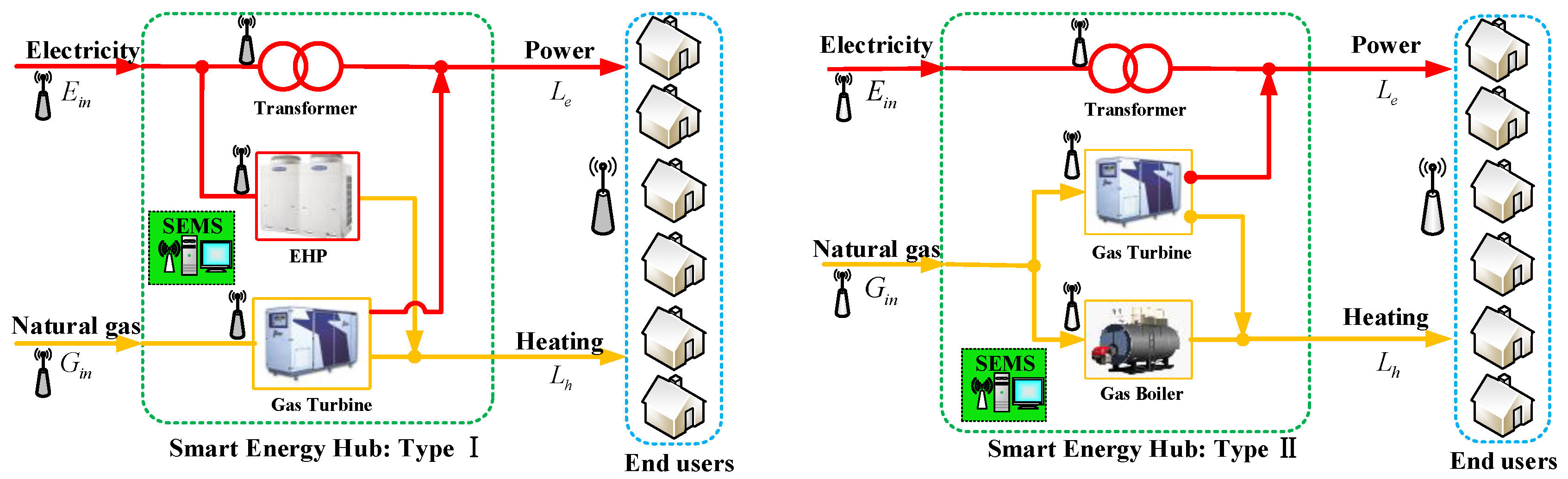
Figure 1 illustrates the architecture of two typical types of smart energy hub. The type I SEH is composed of a gas turbine, electric heat pump, and transformer. The type II SEH is comprised of a gas turbine, gas boiler and transformer. The input ports of the two types of SEH are connected to the electricity and natural gas grids. The output ports can simultaneously provide power and heating energy services to end users. Coupled with power and gas networks and integrating various energy converters, the SEH can consume electricity or natural gas flexibly to satisfy the diversified energy demands of end consumers.
From the perspective of integrated energy suppliers, the energy hubs are immediate electricity and natural gas consumers. When the electricity tariff is high, the energy hubs tend to consume more natural gas, and vice versa. Thus, the electricity load demand from the electricity utility can be reduced in peak periods and increased in valley hours by optimizing the multiple input energy carriers. For the end energy consumers, they are fed by the output energy of energy hubs immediately. Thus, their thermal demands can be provided by the energy hubs instead of their air conditioners. Also, their hot water and heating loads can be supplied by the energy hubs without working their water heaters and heat pumps. Equivalently, the electricity demands are effectively reduced. Thus, from the viewpoint of end energy users, their power and heating demands can be satisfied without changing their electricity consumption behaviors and violating their comfort levels. Of course, the conventional demand response programs (e.g., energy shifting) still work. Thus, in an integrated demand response (IDR) program, energy consumers cannot only shift or curtail their energy consumption, but can also switch the consumed energy type. By taking advantages of complementarities of multi-energy carriers, the IDR becomes more flexible, economic and potential.
Take the input power of each energy converter as variables, then energy flows of the type I SEH can be described by (1) and (2), and the type II SHE can be formulated as (3) and (4).
[ L n , t e L n , t h ] = [ η n T 0 η n G T , e 0 C O P n E H P η n G T , h ] [ E n , t T E n , t E H P G n , t G T ]  
{ E n , t i n = E n , t T + E n , t E H P , G n , t i n = G n , t G T 0 E n , t i n E n i n ¯ , 0 G n , t i n G n i n ¯ 0 E n , t T E n T ¯ , 0 E n , t E H P E n E H P ¯ 0 G n , t G T G n G T ¯  
[ L n , t e L n , t h ] = [ η n T η n G T , e 0 0 η n G T , h η n G B ] [ E n , t T G n , t G T G n , t G B ]  
{ E n , t i n = E n , t T , G n , t i n = G n , t G T + G n , t G B 0 E n , t i n E n i n ¯ , 0 G n , t i n G n i n ¯ 0 E n , t T E n T ¯ , 0 G n , t G T G n G T ¯ 0 G n , t G B G n G B ¯  
A part of the power and heating loads of end users is flexible, thus, it can be shifted or adjusted according to demand response signals. In this paper, the energy shifting of power and heating loads are considered and can be expressed as follows [31].
{ ( 1 R x ) L n , x 0 , t L n , x d r , t ( 1 + R x ) L n , x 0 , t t = 0 T L n , x d r , t = t = 0 T L n , x 0 , t  
where x { e , h } is the index of load type, e and h denote electricity and heating load, respectively, R x denotes the load shifting ratio; the first term of Equation (5) denotes that the load shift should keep within its limits, the second term of Equation (5) denotes the sum of load demands that are not changed after the demand response, L n , x d r , t and L n , x 0 , t are the load x after and before demand response, respectively.

3. The System Model

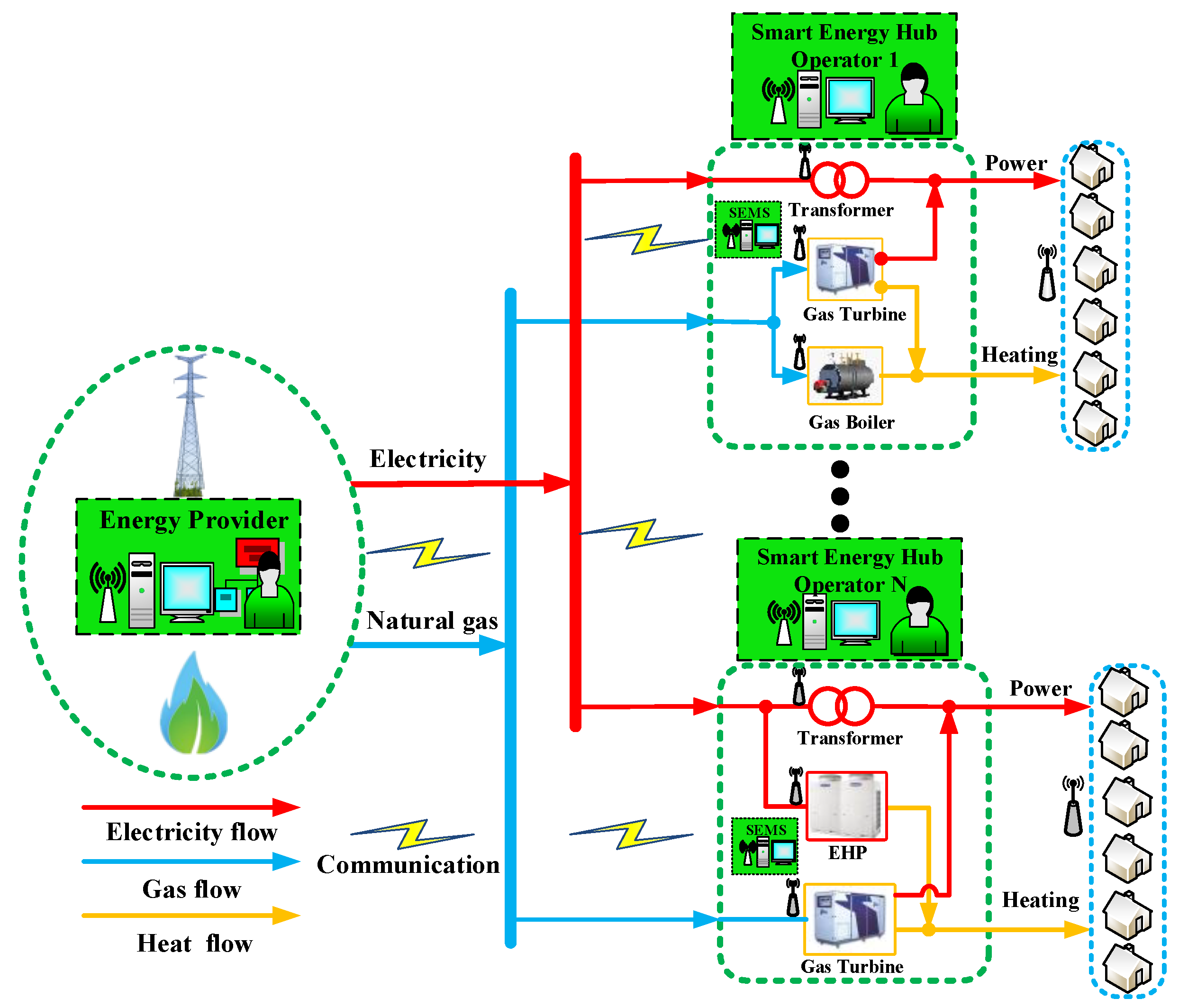
Figure 2 illustrates a smart integrated energy system consisting of one integrated energy provider and N smart energy hub operators (SEHO). The energy provider might be an energy retailer or an alliance of electricity and natural gas utility companies. The energy provider purchases electricity and natural gas from the wholesale market and sells them to the smart energy hub operators in a retail market. Each smart energy hub is equipped with two-way communication infrastructure, smart energy meters and smart energy management system. Bi-directional communication is available between the energy provider and a cluster of SEHOs through a local area network (LAN).
In general, the SEHO is responsible for the normal operation of the SEH and the energy consumption management of end users. One of the most important tasks for the SEHOs is to accurately forecast the power and heating aggregate load demands. Once information has been received, such as the aggregate load demand, the electricity and natural gas prices broadcasted by the energy supplier, then the SEHOs will decide the amount of purchased electricity and natural gas from the energy provider, and coordinate the operation of energy conversion devices to meet the load demands of end users and maximize their revenues.
An integrated demand response program is implemented in this integrated energy system, the real-time electricity and natural gas prices are broadcast to all the SEHOs by the IEP to encourage them to optimize energy consumptions. In the following sections, a more detailed interaction model between one energy provider and a cluster of smart energy hubs will be introduced.

3.1. Integrated Energy Provider Model

The integrated energy provider is assumed to be an alliance of ab electricity utility company and a natural gas utility company. It can supply the electricity and natural gas to energy hubs simultaneously. In general, the energy supply cost is a monotonically increasing function of the amount of supplied energy. Without losing generality, a quadratic function is taken to formulate the energy cost at time slot t [9,10].
C t ( g t ) = a t X ( g t ) 2 + b t X g t + c t X , a t X > 0  
where a t X , b t X and c t X are cost coefficients, which can be predetermined by the energy provider. The g t is the total electricity E t t o or the total natural gas G t t o supplied by the energy provider at time slot t . It is obvious that the energy cost function is strictly convex.
In the IDR program, the real-time electricity price p e , t and the real-time gas price p g , t are determined by the difference in supply and demand, which are broadcast to the smart energy hub operators by the energy provider to encourage them to adjust their energy consumption behaviors.
The payoff U E P t o ( E t t o , G t t o ) of energy provider during a day time can be defined as a function of E t t o and G t t o :
U E P t o ( E t t o , G t t o ) = E t t o p e , t + G t t o p g , t C t ( E t t o ) C t ( G t t o )  
where E t t o p e , t and G t t o p g , t are the profits from selling electricity and natural gas to the energy hub operators at time slot t , respectively. C t ( E t t o ) and C t ( G t t o ) are the electricity supply cost and natural gas supply cost at time slot t , respectively.
Once the real-time energy prices p e , t and p g , t are determined, the energy provider aims to supply the smart energy hub operators a certain amount of electricity and natural gas to maximize his profits. The optimal strategy profiles of the energy provider can be obtained by solving the following optimization problem ((8)–(9)):
( E t t o , G t t o ) * = arg max ( U E P t o ( E t t o , G t t o ) )  
s . t . { n N E n , t i n E t t o E t , max t o n N G n , t i n G t t o G t , max t o  
The constraint (9) guarantees that the electricity and gas supplied by the energy provider can meet the demands of all the energy hub operators. N = [ 1 , , n , , N ] denotes the set of smart energy hub operators. The energy pricing mechanism based on the supply and demand will be discussed in detail in Section 3.3.

3.2. The Smart Energy Hub Operator Model

The utility function of each smart energy hub operator n can be expressed as:
U n ( E n , t i n , G n , t i n ) = ω n , t ( E n , t i n ) E n , t i n p e , t ω n , t ( G n , t i n ) G n , t i n p g , t  
where E n , t i n p e , t and G n , t i n p g , t are the payments of operator n for consuming electricity E n , t i n and natural gas G n , t i n at time t , respectively. ω n , t ( E n , t i n ) and ω n , t ( G n , t i n ) denote the benefits for the satisfaction of energy consumption. Without losing generality, a quadratic function can describe the benefits gained by consuming electricity or natural gas [9,10].
ω n , t ( X n , t i n ) = α n , t X X n , t i n β n X 2 ( X n , t i n ) 2 α n , t X > 0 β n X > 0  
where X n , t i n can be E n , t i n or G n , t i n . Besides, α n , t X is a consumer preference parameter characterizing customer types, which may vary with different consumers and time slots. It can be seen that the consumer with a greater α n , t X prefers to consume more X n , t i n to improve the satisfaction level of energy consumption, and β n X is a predetermined constant.
Each smart energy hub operator optimizes their energy consumption strategies E n , t i n and G n , t i n to maximize their utility and meet the end-use energy demands, which can be obtained by solving the following optimization problems.
{ ( E n , t i n , G n , t i n ) * = arg max [ U n ( E n , t i n , G n , t i n ) ] s . t . ( 1 ) ,   ( 2 ) ,   ( 5 )   o r   ( 3 ) ,   ( 4 ) ,   ( 5 )  

3.3. The Energy Pricing Mechanism: Stackelberg Game Approach

With the further expansion of business, the traditional utility company has become an integrated energy provider, which can provide multi energy resources such as electricity, natural gas, fresh water, etc. to energy consumers. As illustrated in Figure 2, the energy provider simultaneously provides electricity and natural gas to N smart energy hub operators. Meanwhile, the energy provider is the electricity and natural gas price setter. Through setting the electricity and gas prices, the energy provider aims to balance the supply and demand as well as maximize their profits. When the energy prices are broadcast to the SEHOs, the SEHOs will optimize their energy consumption and determine the electricity and natural gas demands to maximize their energy consumption satisfaction. In contrast, the constraint (9) shows that the adjusted energy demands of SEHOs will affect the amount of electricity and gas supplies of the energy provider. In other words, the energy provider can use the energy price as a weapon to induce the smart energy hub operators to participate in the IDR programs as well as keep the energy supply and demand balance.
The interactions between the IEP and SEHOs can be described with the Stackelberg game, where the IEP acts as the leader, and the SEHOs are the followers. A classic game has three elements, the players, the strategy sets and the utility or payoff functions. The one-leader, and N-followers Stackelberg game G S captures the interactions between the IEP and SEHOs and can be formally identified as follows.
G S = { E P N ; Ω E P , Ω n N ; U E P t o , U n }  
• Players E P N :
The energy provider (EP) acts as the leader and the SEHOs in set N = [ 1 , , N ] are followers in response to the strategies of the energy provider.
• Strategy sets Ω E P and Ω n N :
Ω E P = { ( E t t o , G t t o ) | n N E n , t i n E t t o E t , max t o , n N G n , t i n G t t o G t , max t o } denotes the feasible strategy set of the energy provider referring to (9), from which the energy provider determines their energy supply strategy ( E t t o , G t t o ) , namely, the daily electricity and natural gas supply vectors. Each SEHO will select their strategies ( E n , t i n , G n , t i n ) from the feasible strategy set Ω n = { ( E n , t i n , G n , t i n ) | s . t . ( 1 ) , ( 2 ) , ( 5 ) o r ( 3 ) , ( 4 ) , ( 5 ) } , which is defined by constraints (1), (2), (5) or (3), (4), (5).
• Utility or payoff functions U E P t o and U n :
The payoff function U E P t o of IEP denotes the profits gained by selecting the strategy ( E t t o , G t t o ) , and the utility function U n describes the revenue of selecting the strategy ( E n , t i n , G n , t i n ) for each SEHO. It is obvious that the objectives of the IEP and each SEHO are to maximize their benefits (7) and (10), respectively, through adjusting their strategies.
Definition 1.
Let ϕ denote the strategy vector of the energy supplier and ρ denote the strategy vector of all the smart energy hub operators. If the following conditions are satisfied, the strategy vector ( ϕ , ρ ) will be the Stackelberg equilibrium (SE) of the proposed G S game [10].
U e p t o ( ϕ , ρ ) U e p t o ( ϕ , ρ ) , ϕ Ω E P  
U n ( ϕ , ρ ) U n ( ϕ , ρ n , ρ n ) , ρ n Ω n , n N  
where ρ n denotes the equilibrium strategies of all energy hub operators except energy hub operator n. At the SE, no one will benefit by deviating from his strategies.
Theorem 1.
For the proposed Stackelberg game G S , an unique Stackelberg equilibrium exists between the energy provider and smart energy hub operators if the following conditions are satisfied [10,15].
(1) The strategy set of each player is nonempty, convex, and compact.
(2) Each smart energy hub operator has an unique optimal best-response strategy once informed of the strategies of energy provider.
(3) The game leader energy provider will admit a unique optimal strategy profile, once given the best strategies for all the smart energy hub operators.
The proof progressions of this theorem are given in Appendix A.

3.4. Distributed DR Algorithm and Implementation

To protect the privacy of the integrated energy consumers and reduce the communication pressure [32], a distributed algorithm is developed to determine the strategy profiles of each SEHO and the IEP in the Stackelberg equilibrium (SE). 
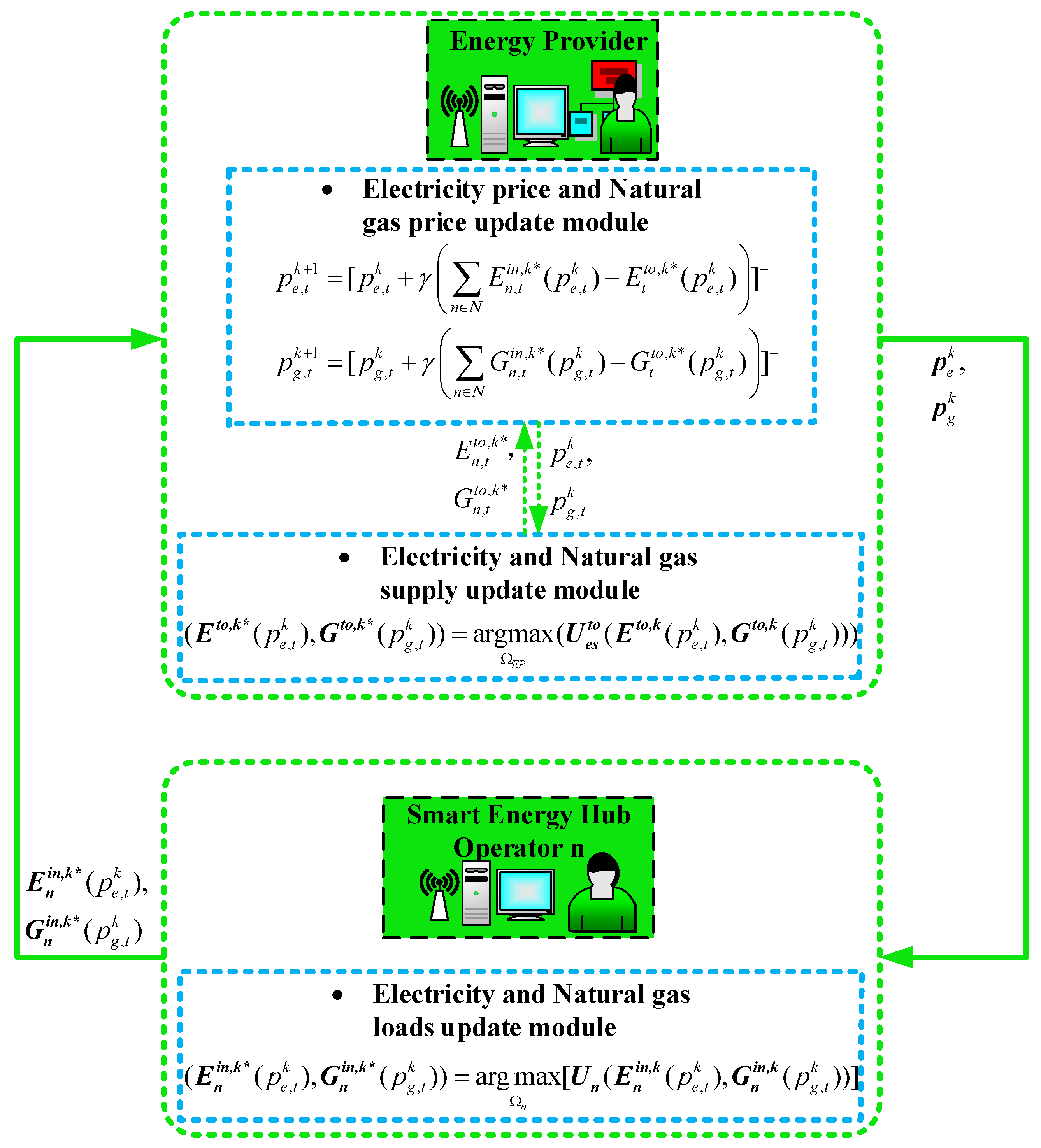
Figure 3 illustrates the interactions between the IEP and the SEHOs when the IDR programs are implemented in the integrated energy system based on the real-time electricity and natural gas prices. Let k denote the iteration number. Let p e , t k and p g , t k denote the electricity price and natural gas price in iteration k at time slot t, respectively. The energy price update module embedded in the smart energy management system of the energy provider is responsible for updating the electricity and gas prices by the following formulas, respectively.
{ p e , t k + 1 = [ p e , t k + γ ( n N E n , t i n * ( p e , t k ) E t t o * ( p e , t k ) ) ] + p g , t k + 1 = [ p g , t k + γ ( n N G n , t i n * ( p g , t k ) G t t o * ( p g , t k ) ) ] +  
where [ ] + is the projection onto the feasible space defined by constraints (1)–(12), γ is the step size, and [[] has proved that there is an upper bound on the step size, a small enough step size can guarantee the convergence, in this paper γ = 10 4 , which is selected by trial and error [33]. More information about the method to choose can be found in [9].
Actually, the energy price update module acts in the coordinator role between the energy provider and smart energy hub operators. As shown in Figure 3, in each iteration at time slot t, the energy price update module of the energy provider updates the prices p e , t k , p g , t k according to the strategies of the energy provider and all the smart energy hub operators, and then broadcasts them to each smart energy hub operator and the energy supply update module. When the prices are received, each smart energy hub operator will update their energy consumption strategies E n i n , * ( p e , t k ) and G n i n , * ( p g , t k ) , and send them back to the energy provider for updating the energy supply strategies E t o , * ( p e , t k ) and G t o , * ( p g , t k ) .
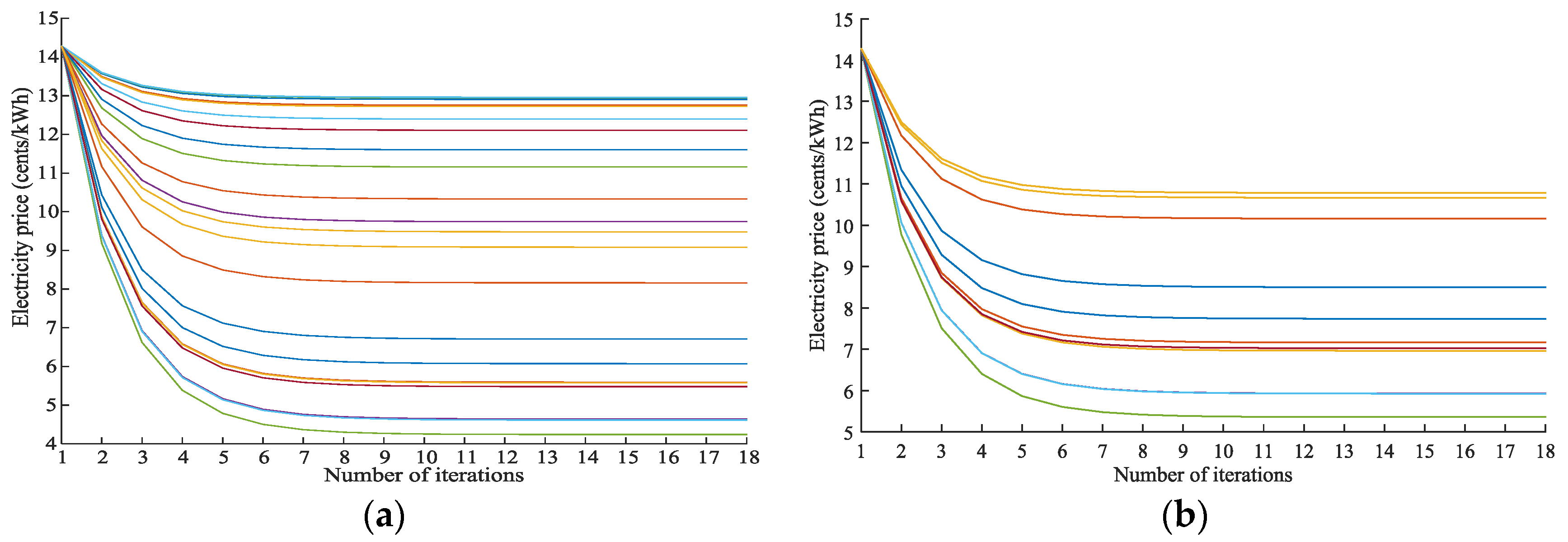
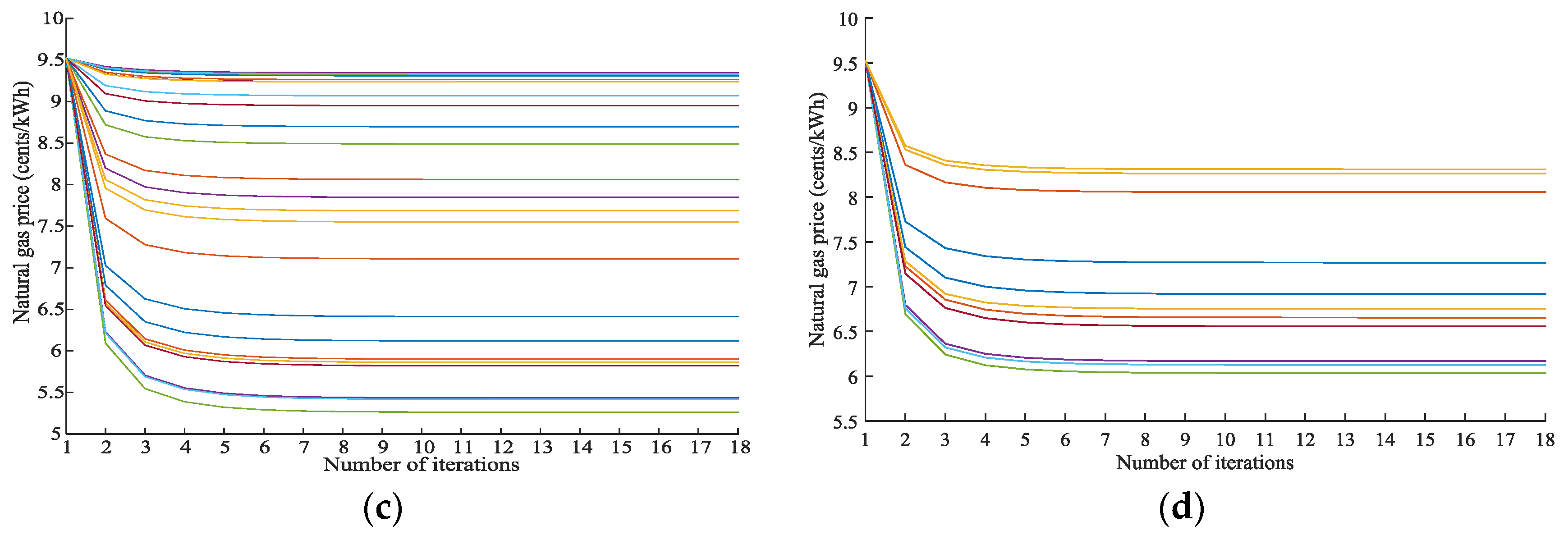
The distributed algorithm is summarized in Algorithm 1. The first line is the initialization. δ denotes the iteration precision, p e 0 and p g 0 are the initial electricity and gas prices, respectively. The loop in lines 2–9 describe the interactions between the energy provider and the smart energy hub operators at each time slot t. In line 5, each smart energy hub receives the electricity price p e , t k and gas price p g , t k broadcasted by the energy provider. In line 6, each smart energy hub updates its optimal energy demands E n i n , * ( p e , t k ) and G n i n , * ( p g , t k ) according to (12), and sends them back to the energy provider while line 8 shows that the energy provider will update its optimal energy supply E t o , * ( p e , t k ) and G t o , * ( p g , t k ) by solving (8)–(9). Once the energy supply and energy demand strategies have been received, the energy price update module of the energy provider will update the electricity price p e , t k and natural gas price p g , t k . In line 10, the iteration number k is updated and the stopping criterion for the algorithm is given in line 11. It is obvious that when the energy supply equals the energy demand, the energy prices will converge. That is to say, the algorithm guarantees the balance of energy supply and demand. Also, at each time slot, the real-time energy prices, the optimal energy supply and consumption strategies will be determined.
Algorithm 1: An iterative algorithm executed by the EP and SEHOs
1: Initialization: k = 0 ,   δ = 10 5 ,   p e 0 ,   p g 0 .
2: While t = T T
3: Repeat
4: For each SEHO n
5: Receive the new electricity price p e ,   t k and gas price p g ,   t k broadcasted by energy provider.
6: Update the electricity consumption value E n ,   t i n , k * and gas consumption value G n ,   t i n , k * according to (12), and send them back to the energy provider.
7: End for
8: Update the amount of electricity supply E t t o , k * and the natural gas supply G t t o , k * amount by solving (8)–(9).
9: Update the electricity price p e , t k and natural gas price p g , t k according to (16).
10: k= k+1.
11: Until max ( | p e , t k + 1 p e , t k | , | p g , t k + 1 p g , t k | ) < δ .
12: End while.

4. Case Studies

4.1. Basic Parameters

In this section, a smart integrated energy system consisting of one integrated energy provider and four smart energy hubs are taken as an example to evaluate the performance of the proposed integrated demand response program. The first two smart energy hubs are assumed as type II, and the last two smart energy hubs are assumed as type I. Each smart energy hub is managed by one smart energy hub operator and is responsible for satisfying the power and heating demands of one residential community which accommodates about 500 persons. The simulation time cycle is divided into T = 24 time slots which represents 24 h of a day. Assume the hourly aggregate power loads L n , e , t and heating loads L n , h , t of each smart energy hub obey the normal distribution,   L n , e , t ~ N ( μ e , t ,   δ e 2 )   ,   L n , h , t ~ N ( μ h , t ,   δ h 2 )   [34]. The hourly aggregate power loads and heating loads of all the smart energy hubs are generated randomly from the normal distribution. The hourly mean parameters μ e , t and μ h , t are given in Figure 4. The standard deviation parameters for aggregate power loads and heating loads are 40 kW and 30 kW, respectively. The parameters of the two types of smart energy hubs are given in Table 1 and all the parameters are chosen randomly from their corresponding intervals.
The coefficients α n , t E for the type I and type II smart energy hubs were chosen randomly from [4,5] and [2.5, 3.5], respectively. The coefficients α n , t G for the type I and type II smart energy hubs were chosen randomly from [3,4] and [4.5, 5.5], respectively. Two cases were considered, the energy shifting of aggregate power and heating loads of end users was not considered in case 1, but were considered in case 2. β n E and β n G for all the SEHs are 0.0025 and 0.002, respectively. a t E = 1 × 10 4 , a t G = 0.6 × 10 4 , b t E = b t G = 0 , c t E = c t G = 0 , δ = 1 × 10 4 , R x = 0.2 . The other parameters of the two types of energy hubs are given in Table 2.

4.2. Simulation Results and Discussions

4.2.1. Real-Time Energy Prices and Load Profiles

Figure 5 illustrates the power and gas prices before and after demand response. Figure 6 shows the aggregated electricity and natural gas loads provided by the energy provider before and after DR (Equation (5)), respectively. It can be seen that the energy prices vary with real time, proportional to the aggregated energy demands during that hour.
Figure 7 and Figure 8 show the purchased power and the purchased gas for each SEH, respectively. Also, the power and gas demand for each SEH are shifted from peak hours to off-peak hours. This is because, before the implementation of the demand response, the energy prices during peak hours are high; when the demand response is employed, all the four energy hub operators will change their energy demands, some peak loads are shifted to off-peak hours. As a result, the energy demands reduce during peak hours and increase during off-peak hours. The energy prices also vary with the total energy demands.
Besides, Figure 9 illustrates the hourly energy supply and demand of the whole integrated energy system before and after the demand response. It is clear that the supply and demand stays balanced at each time slot. This is because the pricing method in (16) can guarantee the supply and demand balance. The results demonstrate the effectiveness of this pricing method, and the integrated demand response also performs well in peak-load shifting.

4.2.2. Comparisons of the Peak-to-Average Ratio (PAR)

The energy provider can benefit from reducing the peak-to-average ratio (PAR) of the aggregated load demands. The PAR of electricity and natural gas provided by the energy provider can be expressed as:
PAR E = max E t t o t T E t t o / T , PAR G = max G t t o t T G t t o / T  
Table 3 gives the PAR of loads before and after the demand response. If all of the energy hubs do not implement the demand response programs, the PAR for the electricity and natural gas loads of the energy provider is 1.370 and 1.214, respectively. If the demand response programs are applied to their end users, the PAR for the electricity loads of the energy provider is reduced to 1.143, about 16.57% less, and the PAR for the natural gas loads of the energy provider is reduced to 1.077, about 11.29% less. Thus, the profiles of electricity and natural gas loads become smooth, which demonstrates that the integrated demand response has an advantage in smoothing the load profiles.

4.2.3. The Convergence of the Demand Response Algorithm

Figure 10 shows the convergence processes of the electricity and gas prices without or with demand response of the end users. In each iteration, the IEP adjusts its energy supply strategies according to the energy consumption strategies of SEHOs, while the SEHOs adjust their energy consumption based on the real-time prices. According to (16), the interactions will stop when the supply and demand balance is satisfied. It can be seen from the results that the demand response algorithm converges very fast. The energy prices converge within 10 iterations.
Figure 11 shows the convergence processes of the payoffs of energy hubs and the cost of the energy provider. The payoffs and cost all converge within 10 iterations. Besides, the payoffs of all energy hubs will increase by considering the demand response and the cost of the energy provider will decrease by considering the demand response. Specifically, the payoffs of EH1, EH2, EH3 and EH4 before implementing the demand response are $74,307.52, $50,946.09, $67,747.64 and $55,291.27 respectively. When consider the demand response, the payoffs increase to $78,812.14, $55,352.93, $72,796.12 and $60,554.23, respectively. Additionally, the operation costs of the energy provider decrease from $48,150.61 to $46,005.76 by considering demand response. Thus, both the energy hub operators and energy providers can benefit from the integrated demand response. As discussed above, the pricing mechanism has a good convergence performance.
Figure 12 illustrates the deviations in energy prices (defined in line 11 of Algorithm 1) between two iterations at time slot 13, the deviation meets the iteration precision at the 10th iteration. When the iteration precision is satisfied, the energy prices are convergent, and the energy supply and demand is balanced. The game reaches equilibrium, neither the energy provider nor the energy operators will change their strategies. The deviations in energy prices for other time slots show the similar patterns.

5. Conclusions

In this paper, a real-time pricing scheme for energy management between one integrated energy provider and multiple energy hub operators was proposed. The interaction between the energy provider (leader) and energy consumers (follower) was formulated as a 1-leader and N-follower game. An interactive algorithm was proposed to derive the Stackelberg equilibrium, through which the best strategies of for energy provider and each energy hub operator are determined to maximize their own benefits. Moreover, the existence and uniqueness of the Stackelberg equilibrium have been proved.
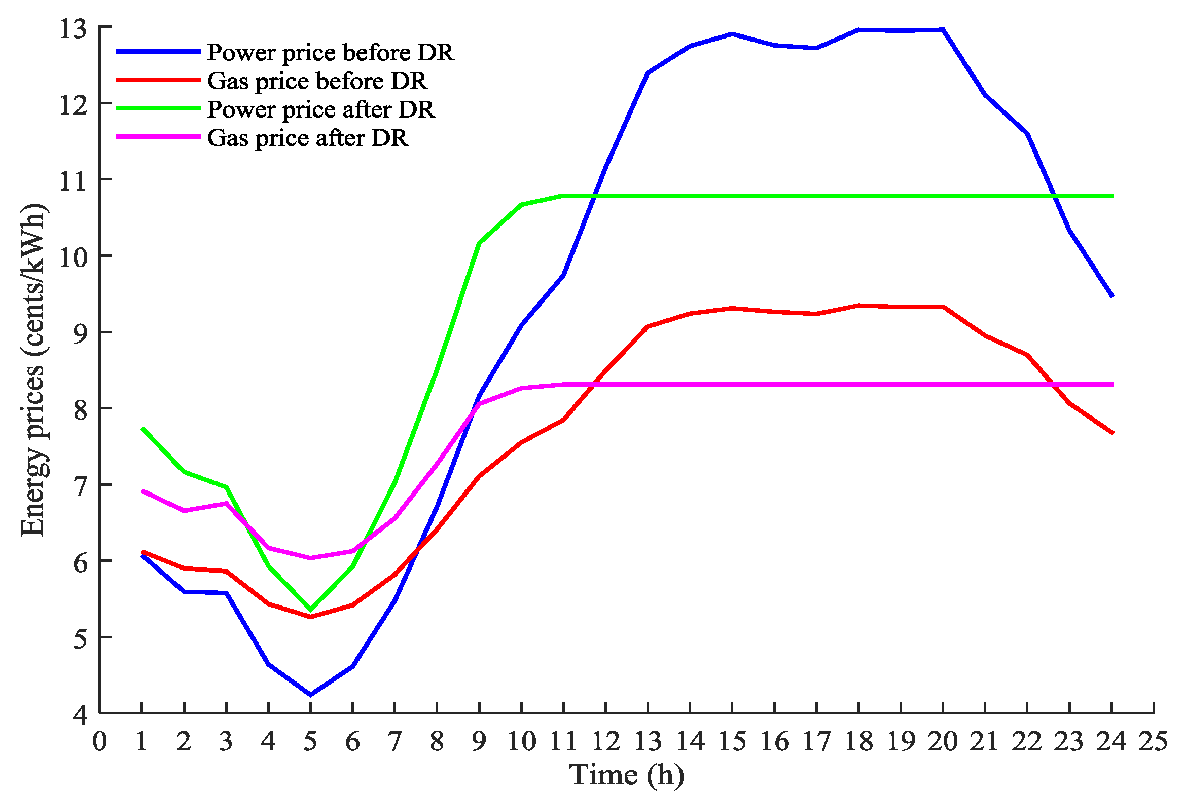
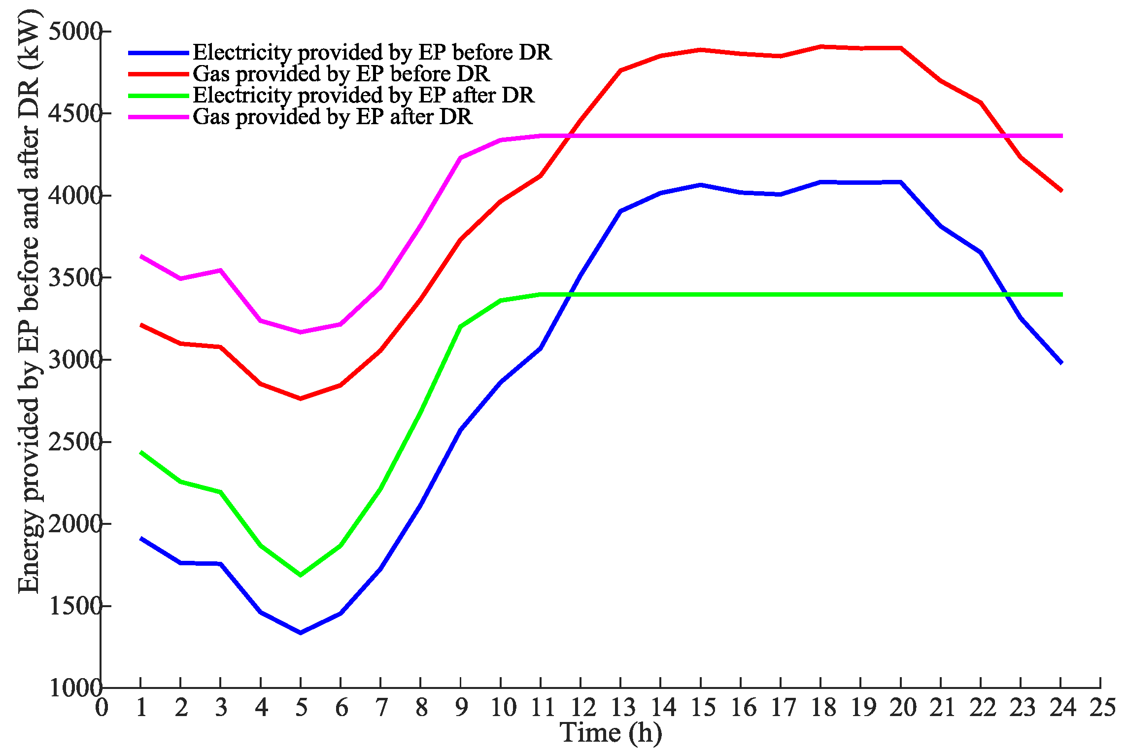
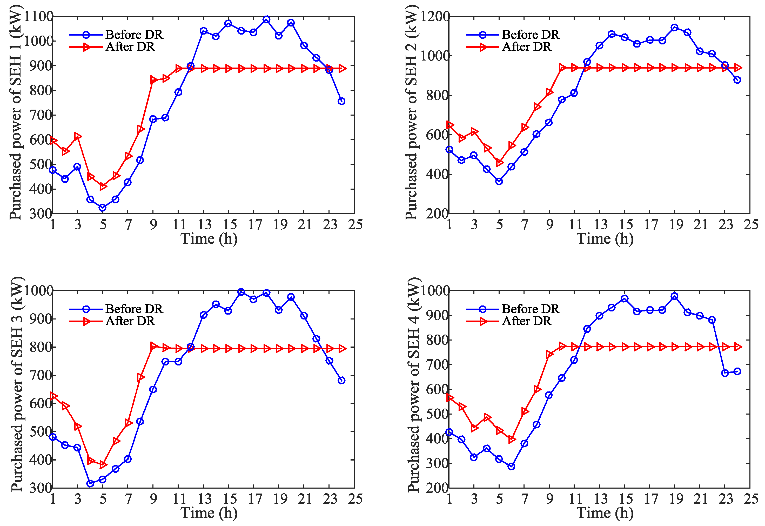
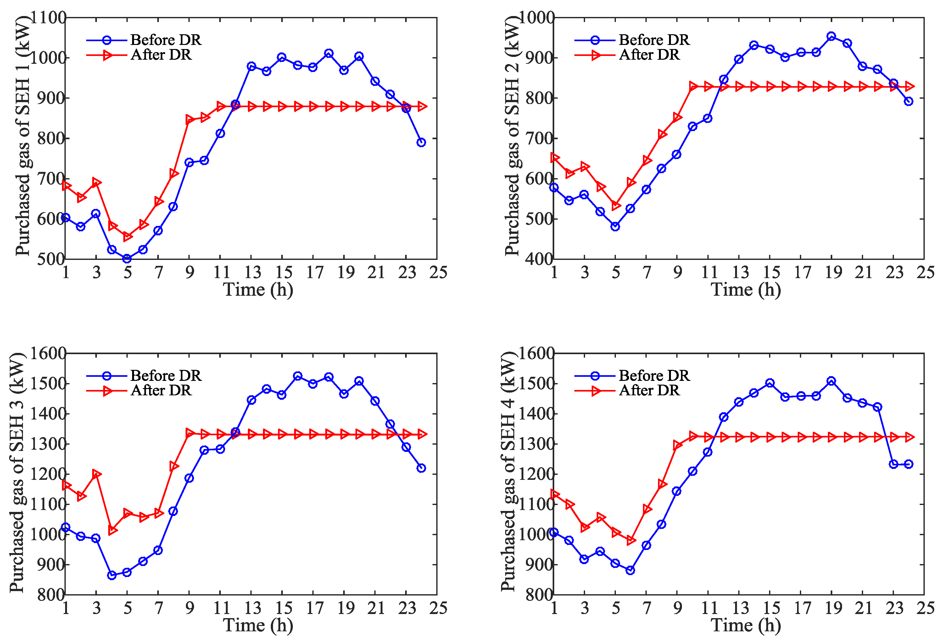
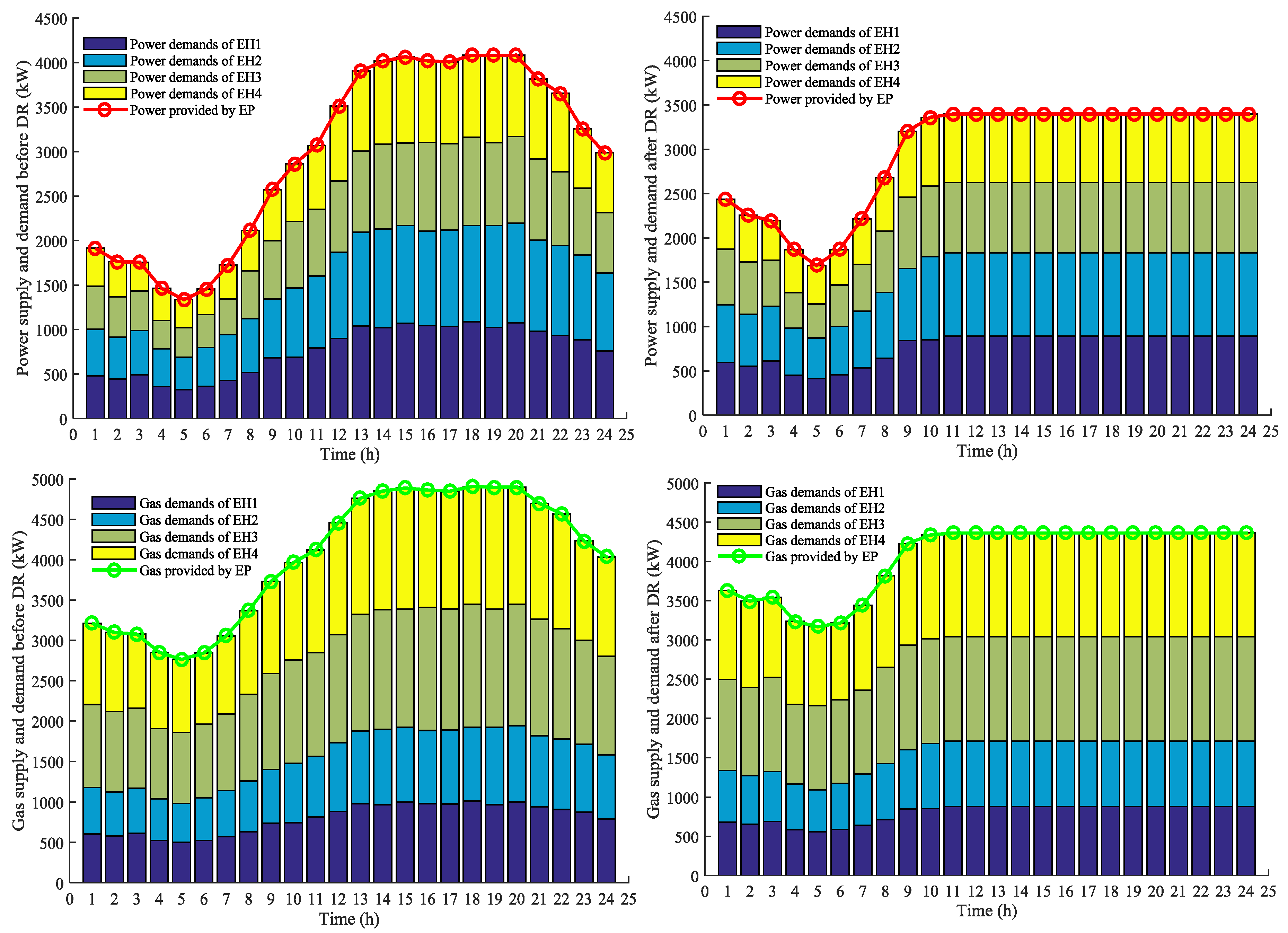
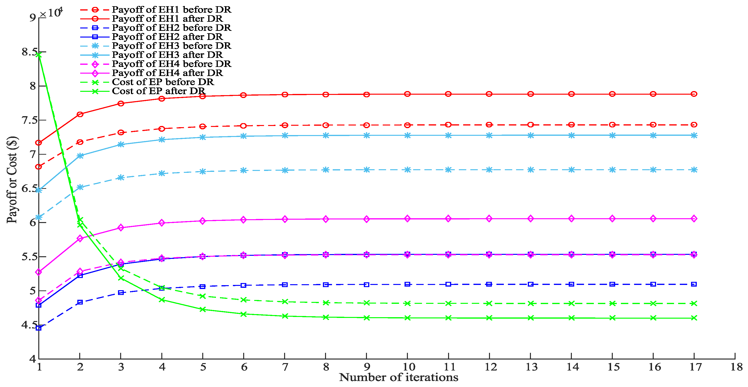
Numerical results showed that the proposed demand response method based on the Stackelberg game can describe the interactions between the IEP and SEHOs and balance the energy supply and demand. Besides, this method can also improve the payoffs for players, as well as smooth the aggregated load profiles for all energy consumers. Furthermore, the pricing method has a good convergence performance and the error was no more than 10 5 .
Renewable energy and energy storage devices were not considered in this paper, which could be considered as an extension of the current work. Also, more specific models of power or heating loads could be considered and discussed in future work.

Author Contributions

T.M. performed the experiments, carried out the theoretical analysis and wrote the paper. J.W. determined the direction of the research and revised the paper and provided important comments on the paper’s structure. L.H. corrected the language and format of the paper. The last two authors (H.Y. and D.L.) are partners in the article’s project.

Funding

This research was funded by the Fundamental Research Funds for the Central Universities [No. E17JB00160], a scholarship from the China Scholarship Council (No. 201707090044) and a technology project of State Grid [No. YDB17201700249].

Conflicts of Interest

The authors declare no conflicts of interest.

Nomenclature

SEHOSmart energy hub operator
EPEnergy provider
SEHSmart energy hub
SEMSSmart energy management system
DRDemand response
TTransformer
EHPElectric heat pump
GTGas turbine
GBGas boiler
n Index of SEH
t Index of time slot
x Index of load type
e / h Electricity/heating load
X { E , G } Index of electricity or gas
T T The set of time slots
a t X / b t X /   c t X Cost coefficients of EP
a n , t X / β n X Preference parameter of SEHO
E n , t i n / G n , t i n Electricity/gas purchased by SEH n
E n , t T / E n , t E H P Power consumed by T/EHP
G n , t G T / G n , t G B Gas consumed by GT, GB
L n , t e / L n , t h power/heating load
η n T / η n G B Efficiency of T/GB
η n G T , e / η n G T , h Electrical/heating efficiency of GT
C O P n E H P Coefficient of performance of EHP
p e , t / p g , t Real time power/gas price
R x Load shifting ratio
L n , x d r , t / L n , x 0 , t Load x after/before DR
E t t o / G t t o Total electricity/natural gas supplied by EP
E t , m a x t o / G t , m a x t o Maximum electricity/natural gas supplied by EP
γ Step size

Appendix A

Proof of Theorem 1:
Proof 1.
The sets Ω n and Ω E P defined in (1)–(5) and (9) are linear equality (i.e., constraints (1), (3), (5)) and convex constraints (i.e., constraints (2), (4), (5) and (9)). These sets are obviously defined as nonempty, convex and compact [35].
Proof 2.
Once the strategies of the energy provider are received, the best response functions can be directly obtained through taking the first order partial derivative of U n ( E n i n , G n i n ) with respect to E n , t i n and G n , t i n , respectively.
U n E n , t i n = a n , t E β n , t E E n , t i n p e , t  
U n G n , t i n = a n , t G β n , t G G n , t i n p g , t  
The second order partial derivative of U n ( E n i n , G n i n ) can be calculated as follows.
2 U n E n , t i n 2 = β n , t E  
2 U n G n , t i n 2 = β n , t G  
2 U n E n , t i n G n , t i n = 0 , 2 U n G n , t i n E n , t i n = 0  
The Hessian matrix:
H ( U n ) = [ 2 U n E n , t i n 2 2 U n E n , t i n G n , t i n 2 U n G n , t i n E n , t i n 2 U n G n , t i n 2 ]  
Since β n , t E > 0 , β n , t G > 0 , then the value of (A3) and (A4) are always negative; therefore, all the diagonal elements of H ( U n ) are negative; all the off-diagonal elements are zeros, thus all the principal minors become negative, and then the hessian matrix is negative definite. Therefore, the payoff function U n ( E n i n , G n i n ) is strictly concave in Ω E P . Thus, each smart energy hub operator will have a unique optimal best-response strategy once the strategies of the energy supplier is announced.
Proof 3.
Once the optimal strategies of all the smart energy hub operator have been determined, the Ω n is convex. Because the energy cost function C t ( g t ) is strictly convex, so if given the energy prices p e , t and p g , t , the utility function U e s t o ( E t o , G t o ) in (7) is strictly concave. Therefore, the optimization problem described by (8) and (9) is a convex optimization problem and it has a unique solution [9,35]. Thus, the game leader energy supplier will disclose a unique optimal strategy when given the best strategies of all the energy hub operators.

References

  1. Lund, H.; Østergaard, P.A.; Connolly, D.; Mathiesen, B.V. Smart energy and smart energy systems. Energy 2017, 137, 556–565. [Google Scholar] [CrossRef]
  2. Tronchin, L.; Manfren, M.; Nastasi, B. Energy efficiency, demand side management and energy storage technologies—A critical analysis of possible paths of integration in the built environment. Renew. Sustain. Energy Rev. 2018, 95, 341–353. [Google Scholar] [CrossRef]
  3. Geidl, M.; Koeppel, G.; Favre-perrod, P.; Klöckl, B.; Andersson, G.; Fröhlich, K. The Energy Hub—A Powerful Concept for Future Energy Systems. In Proceedings of the Third Annual Carnegie Mellon Conference on the Electricity Industry, Pittsburgh, PA, USA, 13–14 March 2007. [Google Scholar]
  4. Dong, J.; Xue, G.; Li, X. Value Evaluation of Integrated Energy Services Based on Balanced Scorecard. In Proceedings of the 2016 International Conference on Humanities and Social Science (HSS 2016), Guangzhou, China, 8–10 January 2016. [Google Scholar]
  5. Samarakoon, K.; Ekanayake, J.; Jenkins, N. Reporting available demand response. IEEE Trans. Smart Grid 2013, 4, 1842–1851. [Google Scholar] [CrossRef]
  6. Kies, A.; Schyska, B.U.; von Bremen, L. The Demand Side Management Potential to Balance a Highly Renewable European Power System. Energies 2016, 9, 955. [Google Scholar] [CrossRef]
  7. Jabir, H.J.; Teh, J.; Ishak, D.; Abunima, H. Impact of Demand-Side Management on the Reliability of Generation Systems. Energies 2018, 11, 2155. [Google Scholar] [CrossRef]
  8. Arteconi, A.; Polonara, F. Assessing the Demand Side Management Potential and the Energy Flexibility of Heat Pumps in Buildings. Energies 2018, 11, 1846. [Google Scholar] [CrossRef]
  9. Bahrami, S.; Sheikhi, A. From Demand Response in Smart Grid Toward Integrated Demand Response in Smart Energy Hub. IEEE Trans. Smart Grid 2016, 7, 650–658. [Google Scholar] [CrossRef]
  10. Yu, M.; Hong, S.H. Supply-demand balancing for power management in smart grid: A Stackelberg game approach. Appl. Energy 2016, 164, 702–710. [Google Scholar] [CrossRef]
  11. Sheikhi, A.; Rayati, M.; Bahrami, S.; Ranjbar, A.M. Demand side management in a group of Smart Energy Hubs as price anticipators; The game theoretical approach. In Proceedings of the 2015 IEEE Power and Energy Society Innovative Smart Grid Technologies Conference, Washington, DC, USA, 18–20 February 2015. [Google Scholar]
  12. Yang, P.; Tang, G.; Nehorai, A. A game-theoretic approach for optimal time-of-use electricity pricing. IEEE Trans. Power Syst. 2013, 28, 884–892. [Google Scholar] [CrossRef]
  13. Ma, J.; Deng, J.; Song, L.; Han, Z. Incentive Mechanism for Demand Side Management in Smart Grid Using Auction. IEEE Trans. Smart Grid 2014, 5, 1379–1388. [Google Scholar] [CrossRef]
  14. Mohsenian-Rad, A.H.; Wong, V.W.S.; Jatskevich, J.; Schober, R.; Leon-Garcia, A. Autonomous demand-side management based on game-theoretic energy consumption scheduling for the future smart grid. IEEE Trans. Smart Grid 2010, 1, 320–331. [Google Scholar] [CrossRef]
  15. Maharjan, S.; Zhu, Q.; Zhang, Y.; Gjessing, S.; Basar, T. Dependable Demand Response Management in the Smart Grid: A Stackelberg Game Approach. IEEE Trans. Smart Grid. 2013, 4, 120–132. [Google Scholar] [CrossRef]
  16. Yang, J.; Zhang, G.; Ma, K. Real-time pricing-based scheduling strategy in smart grids: A hierarchical game approach. J. Appl. Math. 2014, 2014. [Google Scholar] [CrossRef]
  17. Samadi, P.; Mohsenian-Rad, H.; Wong, V.W.S.; Schober, R. Real-Time Pricing for Demand Response Based on Stochastic Approximation. IEEE Trans. Smart Grid 2014, 5, 789–798. [Google Scholar] [CrossRef]
  18. Jalali, M.M.; Kazemi, A. Demand side management in a smart grid with multiple electricity suppliers. Energy 2015, 81, 766–776. [Google Scholar] [CrossRef]
  19. Han, X.; Wang, F.; Tian, C.; Xue, K.; Zhang, J. Economic evaluation of actively consuming wind power for an integrated energy system based on game theory. Energies 2018, 11, 1476. [Google Scholar] [CrossRef]
  20. Hwang, Y.M.; Sim, I.; Sun, Y.G.; Lee, H.-J.; Kim, J.Y. Game-Theory Modeling for Social Welfare Maximization in Smart Grids. Energies 2018, 11, 2315. [Google Scholar] [CrossRef]
  21. Wang, Y.; Huang, Y.; Wang, Y.; Yu, H.; Li, R.; Song, S. Energy Management for Smart Multi-Energy Complementary Micro-Grid in the Presence of Demand Response. Energies 2018, 11, 974. [Google Scholar] [CrossRef]
  22. Liu, X.; Wang, S.; Sun, J. Energy Management for Community Energy Network with CHP Based on Cooperative Game. Energies 2018, 11, 1066. [Google Scholar] [CrossRef]
  23. Yang, H.; Xiong, T.; Qiu, J.; Qiu, D.; Dong, Z.Y. Optimal operation of DES/CCHP based regional multi-energy prosumer with demand response. Appl. Energy 2016, 167, 353–365. [Google Scholar] [CrossRef]
  24. Geidl, M.; Andersson, G. Optimal power flow of multiple energy carriers. IEEE Trans. Power Syst. 2007, 22, 145–155. [Google Scholar] [CrossRef]
  25. Shao, C.; Wang, X.; Shahidehpour, M.; Wang, X.; Wang, B. An MILP-Based Optimal Power Flow in Multicarrier Energy Systems. IEEE Trans. Sustain. Energy 2017, 8, 239–248. [Google Scholar] [CrossRef]
  26. Mohsenzadeh, A.; Ardalan, S.; Haghifam, M.-R.; Pazouki, S. Optimal place, size, and operation of combined heat and power in multi carrier energy networks considering network reliability, power loss, and voltage profile. IET Gener. Transm. Distrib. 2016, 10, 1615–1621. [Google Scholar]
  27. Zhang, X.; Che, L.; Shahidehpour, M.; Alabdulwahab, A.S.; Abusorrah, A. Reliability-Based Optimal Planning of Electricity and Natural Gas Interconnections for Multiple Energy Hubs. IEEE Trans. Smart Grid 2017, 8, 1658–1667. [Google Scholar] [CrossRef]
  28. Sheikhi, A.; Bahrami, S.; Ranjbar, A.M. An autonomous demand response program for electricity and natural gas networks in smart energy hubs. Energy 2015, 89, 490–499. [Google Scholar] [CrossRef]
  29. Bahrami, S.; Toulabi, M.; Ranjbar, S.; Moeini-Aghtaie, M.; Ranjbar, A.M. A Decentralized Energy Management Framework for Energy Hubs in Dynamic Pricing Markets. IEEE Trans. Smart Grid 2017. [Google Scholar] [CrossRef]
  30. Sheikhi, A.; Rayati, M.; Bahrami, S.; Ranjbar, A.M. Integrated demand side management game in smart energy hubs. IEEE Trans. Smart Grid 2015, 6, 675–683. [Google Scholar] [CrossRef]
  31. Alipour, M.; Zare, K.; Abapour, M. MINLP Probabilistic Scheduling Model for Demand Response Programs Integrated Energy Hubs. IEEE Trans. Ind. Inform. 2017, 14, 79–88. [Google Scholar] [CrossRef]
  32. Li, N.; Chen, L.; Dahleh, M.A. Demand Response Using Linear Supply Function Bidding. IEEE Trans. Smart Grid 2015, 6, 1827–1838. [Google Scholar] [CrossRef]
  33. Ma, K.; Hu, G.; Spanos, C.J. Distributed energy consumption control via real-time pricing feedback in smart grid. IEEE Trans. Control Syst. Technol. 2014, 22, 1907–1914. [Google Scholar] [CrossRef]
  34. Kamyab, F.; Bahrami, S. Efficient operation of energy hubs in time-of-use and dynamic pricing electricity markets. Energy 2016, 106, 343–355. [Google Scholar] [CrossRef]
  35. Boyd, S.; Vandenberghe, L. Convex Optimization, 1st ed.; Cambridge University Press: New York, NY, USA, 2004. [Google Scholar]
Figure 1. Two typical types of smart energy hub.
Energies 11 02858 g001
Figure 2. The schematic diagram of a smart integrated energy system consisting of one energy provider and N smart energy hub operators.
Energies 11 02858 g002
Figure 3. Interactions between the energy provider and smart energy hubs.
Energies 11 02858 g003
Figure 4. Mean value of energy loads of each energy hub (EH).
Energies 11 02858 g004
Figure 5. Real time power and gas prices before and after the demand response (DR).
Energies 11 02858 g005
Figure 6. Real time energy supply by the energy provider (EP) before and after DR.
Energies 11 02858 g006
Figure 7. Hourly power demands of all EHs before and after DR.
Energies 11 02858 g007
Figure 8. Hourly gas demands of all EHs before and after DR.
Energies 11 02858 g008
Figure 9. Hourly energy supply and demand of the whole energy system.
Energies 11 02858 g009
Figure 10. The convergence processes of energy prices: (a) The convergence processes of electricity prices without DR; (b) The convergence processes of electricity prices with DR; (c) The convergence processes of gas prices without DR; (d) The convergence processes of gas prices with DR.
Energies 11 02858 g010aEnergies 11 02858 g010b
Figure 11. The convergence processes of payoffs of EHs and cost of EP.
Energies 11 02858 g011
Figure 12. The changes of iteration deviation.
Energies 11 02858 g012
Table 1. Parameters of smart energy hubs.
Smart EH Type η n , T η n , G T e η n , G T h C O P n , E H P η n , G B
Type I[0.95, 0.98]*[0.3, 0.38][0.4, 0.48][2.5, 3.5]
Type II[0.92, 0.96][0.28, 0.33][0.44, 0.5][0.85, 0.95]
1 [a, b]* represents that the parameter obeys the uniform distribution of the range [a, b].
Table 2. Parameters of the devices in the smart energy hubs.
Type I E n T ¯ E n E H P ¯ G n G T ¯
1500 kW500 kWh4000 kWh
Type II E n T ¯ G n i n ¯ G n G B ¯
2000 kW5000 kW1000 kW
Table 3. PAR of loads before and after DR.
ItemsBefore DRAfter DR
PAR of Electricity1.3701.143
PAR of Natural gas1.2141.077

