Optimization of Control Variables and Design of Management Strategy for Hybrid Hydraulic Vehicle

Abstract

The article deals with optimization of control variables and design of management strategy for a hybrid hydraulic vehicle in parallel configuration. Conventionally driven delivery truck with experimentally verified data from the previous research is taken as a starting base and benchmark for comparison of the benefits of hybridization. Optimization of control variables is carried out using dynamic programming (DP) algorithm to gain insight into optimum operation of the driveline and minimum possible fuel consumption for five different driving cycles. Two rule based management strategies are given and compared, one of which is improved and innovative, based on the knowledge gained from DP results. Hybrid driveline can reduce fuel consumption from 5% to 30% depending on the driving cycle. More dynamic cycles with lot of "stop-and-go" events score greater reduction. Innovative management strategy has achieved a similar distribution of internal combustion engine (ICE) operating points as DP optimization but this did not result in a consistent reduction of fuel consumption compared to basic management strategy for all cycles. That is explained by the state of charge (SoC) behaviour and reducing the potential for recovery of regenerative braking energy.

1. Introduction

The rigid legislation on emissions and consumption requirements has made hybrid vehicles more common. However, under hybrid vehicles we regularly imply hybrid electric vehicles (HEV) of different drivetrain configuration (series, parallel, series/parallel) and different content of the electric part (micro, mild, full, plug-in). But there is also a hybrid vehicle niche with hydraulics instead of electric drives and chemical batteries and these are hybrid hydraulic vehicles (HHV). Generally, they come in parallel or series drivetrain configuration and use the hydro-pneumatic accumulators as energy storage elements. The main characteristics of hydro-pneumatic accumulators are their high power density and low energy density, which is just the opposite of the chemical batteries from HEV. That characteristic determines the most common applications of HHV and these are commercial vehicles that operate mainly in stop-and-go regime, like for example shuttle busses, delivery trucks or vans, garbage trucks, tractors in port terminals and similar. Compared to the HEV counterpart the HHV can be more cost effective. The enhancement of performances is similar or even better, the hydraulic elements usually cost less, while the utilized elements are more accessible (“on-the-shelf”) and simpler for maintenance in regular workshops. Moreover, the parallel HHV configuration is simple and the adaptation or retrofitting of the classical driveline to the hybrid hydraulic option often can be made readily. Due to its simplicity and affordability the parallel configuration of HHV is probably the most effective way to consumption and pollution betterment for a certain class of commercial vehicles. The parallel HHV configuration consists of a hydraulic motor/pump unit, hydro-pneumatic accumulator and an internal combustion engine (ICE). A comprehensive overview of the commercial vehicle hybrid technology is given in Reference [1]. A review on the control of HEV is given in Reference [2], while the modelling and optimization of the vehicle propulsion systems from the same authors is given in Reference [3]. An innovative example of a city bus is given in Reference [4] where hydraulics is in synergy with electric drive.

The hybrid vehicle achieves better fuel consumption and pollution results through the regenerative braking, ICE downsizing and possibility of ICE operation in a more favourable region. Hybrid driveline management is a key factor regarding consumption and emissions improvements and that is a topic of this paper. The optimal operating mode of the HHV differs from the HEV because the characteristics of hydraulic and electric components are pretty different. Hence the design of a management strategy of HHV should have different approach than the management strategies developed for HEV drives [5]. However, the optimum mode of operation for a given driveline configuration and components is tested by optimizing control variables, what is the same as with HEV. Dynamic programming algorithm (DP) is most commonly used in this case and it results in globally optimal results [5,6]. There are generally two approaches to the design of management strategies of hybrid vehicle driveline: Rule based (RB) strategy (heuristic) or an optimization-based approach like ECMS (Equivalent Consumption Minimization Strategy) (e.g., [5,7,8,9]). Management strategies constitutes a challenging problem due to the complex structure of a HEV and the unknown or partially known driving cycles. To meet this problem, in Reference [10] a stochastic dynamic programming method is adopted. Other useful research on electric vehicles regenerative braking or field test performance verification is provided in References [11,12]. An overview of different optimization methods applied on the hybrid hydraulic vehicles is given in Reference [13], while the study of parallel HEV potential is presented in Reference [14].

Conventionally driven delivery truck with experimentally verified data from the previous research is taken as a starting base and benchmark for comparison of the benefits of application of hybrid hydraulic drive. A mathematical model of a conventional vehicle (CV) driven by ICE (Diesel engine) of 176 kW is given in Section 2 of this paper. CV model is given in details in Reference [15] and there is also validation in relation to the experimentally collected data. This model is extended here with hydraulic components that include a hydraulic motor/pump and a hydro-pneumatic accumulator in a parallel configuration.

Optimization of control variables is carried out using the DP algorithm to gain insight into optimum operation of the driveline and minimum possible fuel consumption for different driving cycles. That is given in Section 3. Minimum fuel consumption is used later to verify causal management strategies that do not use future knowledge of the cycle.

Finally, in Section 4 two rule based management strategies are given, one of which is improved and innovative, based on the knowledge gained from DP results.

In Section 5 model simulations over different driving cycles give insight into how much fuel consumption can be reduced compared to a conventional vehicle and how much causal management strategies can approach the optimum DP results.

In addition to optimizing the control variables, it would be important for HHV to optimize the driveline configuration and drive components size for the given vehicle and driving cycle in order to take full advantage of the hybridization. The size of the ICE, motor/pump unit, hydro-pneumatic accumulator, its pressure settings, choice of output transmission ratio are considered the most important parameters when sizing the driveline components. However, the sizing of components is out of the scope of this paper. The size of the hydraulic components is taken from the B.Sc. thesis [16], while the size and maps of the conventional driveline are taken from [15].

2. Mathematical Model of Delivery Truck Drivetrain

2.1. Mathematical Model of Conventional Vehicle Driveline

In this paper, the delivery truck MAN TGM 15.240 (load capacity approx. 8 tons) shown in Figure 1 is considered. The quasi-static model of the conventional driveline with the internal combustion engine is given in Figure 2. The driveline includes an automated manual transmission with 12 gear ratios (the gear ratios are given in

Table A1. List of delivery truck, hydraulics and optimization parameters (from [15,16]).

Symbol	Value	Description
Af	9.63 [m2]	Forehead area of vehicle
Cd	0.63 [-]	Drag coefficient
Dmin	−2.38 × 10−5 [m3]	Minimal volume of hydraulic motor/pump
Dmax	2.38 × 10−5 [m3]	Maximal volume of hydraulic motor/pump
g	9.81 [m/s2]	Gravity acceleration
h	10.33, 8.40, 6.49, 5.27, 4.18, 3.40, 2.47, 2.01, 1.55, 1.26, 1, 0.81	Gear ratios
io	3.7 [-]	Output reduction ratio
Kf	105 [-]	Penalization factor in criterion in (23)
Kg	106 [-]	Penalization factor in criterion in (19)
m	14.2 [kg]	Mass of gas in hydro-pneumatic accumulator
mv	7860 [kg]	Vehicle mass
pa	101,300 [Pa]	Ambient pressure
r	0.388 [m]	Effective radius of tire
R	296.8 [J/kg·K]	Specific gas constant
Ro	0.012 [-]	Rolling resistance factor
T	300 [K]	Gas temperature
Vmin	0.05 [m3]	Min. volume of gas in hydro-pneumatic acc.
Vmax	0.1 [m3]	Max. volume of gas in hydro-pneumatic acc.
ηf	0.96 [-]	Mechanical transmission efficiency
ηh-m	0.91 [-]	Hydraulic-mechanical efficiency
ηv	0.95 [-]	Volumetric efficiency
ρair	1.225 [kg/m3]	Air density
Af	9.63 [m2]	Forehead area of vehicle
Cd	0.63 [-]	Drag coefficient
Dmin	−2.38 × 10−5 [m3]	Minimal volume of hydraulic motor/pump
Dmax	2.38 × 10−5 [m3]	Maximal volume of hydraulic motor/pump
g	9.81 [m/s2]	Gravity acceleration
h	10.33, 8.40, 6.49, 5.27, 4.18, 3.40, 2.47, 2.01, 1.55, 1.26, 1, 0.81	Gear ratios
ih	2 [-]	Reduction ratio of joint between hydraulics and mechanical transmission
io	3.7 [-]	Output reduction ratio
Kf	105 [-]	Penalization factor in criterion in (23)
Kg	106 [-]	Penalization factor in criterion in (19)
m	14.2 [kg]	Mass of gas in hydro-pneumatic accumulator
mv	7860 [kg]	Vehicle mass
pa	101,300 [Pa]	Ambient pressure
r	0.388 [m]	Effective radius of tire
R	296.8 [J/kg·K]	Specific gas constant
Ro	0.012 [-]	Rolling resistance factor
T	300 [K]	Gas temperature
Vmin	0.05 [m3]	Min. volume of gas in hydro-pneumatic acc.
Vmax	0.1 [m3]	Max. volume of gas in hydro-pneumatic acc.
ηf	0.96 [-]	Mechanical transmission efficiency
ηh-m	0.91 [-]	Hydraulic-mechanical efficiency
ηv	0.95 [-]	Volumetric efficiency
ρair	1.225 [kg/m3]	Air density

in Appendix A).

Driver demand block from Figure 2 determines the required wheel moment τ_L and its rotational speed ω_L depending on speed v_v and mass m_v of the vehicle based on the following equations:

$${\tau }_L=r\left[m_v\left(\frac{d{v}_v}{dt}+g(\sin \alpha +R_o\cos \alpha )\right)+0.5{\rho }_{air}{C}_d{A}_f{v}_v{}^2\right]$$

(1)

$${\omega }_L=v_v/r$$

(2)

Then, ICE rotational speed ω_e is determined by the differential transmission ratio i_o, wheel rotational speed ω_L and the gear shift transmission ratio h. The transmission ratio h is determined in the Management strategy block in order to minimize fuel consumption and to meet limitations on maximum torque and rotational speed of ICE, differential transmission ratio i_o and wheel rotational speed ω_L. The gear shift transmission ratio h selection is described later in Section 4.2.

$${\omega }_e={\omega }_L{i}_{o}h$$

(3)

The engine torque τ_e is determined by the required wheel torque τ_L and transmission ratios i_o and h and taking into account the transmission efficiency η_f:

$${\tau }_e=\frac{{\tau }_L}{{\eta }_f{i}_{o}h}$$

(4)

The fuel flow dm_f/dt is calculated from the specific fuel consumption map shown in Figure 3 based on the following Equation:

$${\dot{m}}_f({\tau }_e,{\omega }_e)=\frac{{\tau }_e{\omega }_e{\overline{m}}_f({\tau }_e,{\omega }_e)}{1000·3600}[\mathrm{g}/\mathrm{s}]$$

(5)

The total fuel consumption (expressed in liters) is obtained by integrating the fuel flow as follows:

$$V_{f,tot}=\frac{1}{850}{{\displaystyle \int }}_{t=0}^{T_f}{\dot{m}}_f({\tau }_e,{\omega }_e)dt\hspace{1em}[\mathrm{L}]$$

(6)

where T_f denotes the total duration of the driving cycle. Integral is scaled by 850 due to the fuel density (≈850 g/dm³).

In Figure 3 the specific consumption map and the maximum torque curve is given for the particular Diesel ICE employed in the delivery truck MAN TGM 15.240. Note that the minimum rotational speed at which the engine can operate is slightly greater than 100 rad/s.

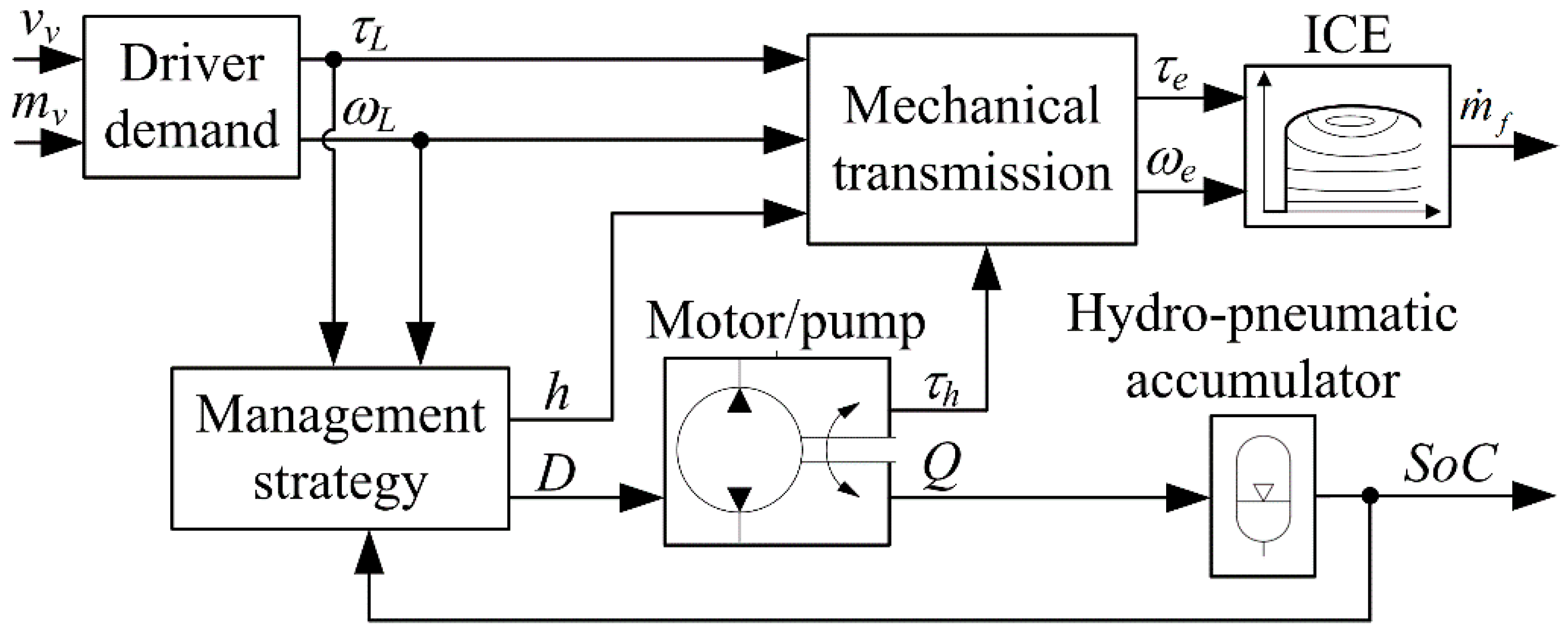
2.2. Mathematical Model of Parallel Hybrid Hydraulic Vehicle Driveline

The hybrid hydraulic vehicle (HHV) driveline mathematical model is obtained by adding a hydromotor/pump and a hydro-pneumatic accumulator to a conventional vehicle (CV) driveline model. The HHV parallel configuration is depicted in Figure 4. The hydro-pneumatic energy storage consists of a high-pressure accumulator (HPA) and a low pressure accumulator (LPA, could be atmospheric tank, as well). The hydraulic fluid (usually mineral oil) compresses gas (usually nitrogen) in accumulator and the compressed gas actually stores energy (like a spring). The hydraulic fluid goes from LPA to HPA (saving energy) when the hydraulic unit works as a pump (during braking) and in reverse direction, from HPA to LPA (wasting saved energy), when the hydraulic unit works as a motor (during acceleration). An explanation of the operation of the parallel HHV is illustrated for example in Reference [17].

The block diagram of the quasi-static mathematical model of parallel HHV is shown in Figure 5 and is obtained by expanding the model shown in Figure 2. In addition to the optimum transmission ratio h, the Management strategy block determines the volume of the motor/pump D, which is the control variable related to the hydraulic part of the driveline.

The volume of the motor/pump D determines its torque τ_h and related fluid flow Q in hydraulic circuit according to following terms:

$${\tau }_h=D\left(p-p_a\right),\hspace{1em}{D}_{\mathit{min}}\le D\le D_{\mathit{max}}$$

(7)

$$Q=\{\begin{array}{c}D·{\omega }_h·\frac{1}{{\eta }_v},\hspace{1em}D\ge 0\\ D·{\omega }_h·\frac{1}{{\eta }_v},\hspace{1em}D<0\end{array}$$

(8)

η_v means volumetric efficiency of hydraulic motor/pump and ω_h is its rotational speed. It depends on wheel rotational speed ω_L and reduction ratio i_h of a joint between hydraulics and mechanical transmission using following Equation:

$${\omega }_h={\omega }_L{i}_o{i}_h$$

(9)

p and p_a denote fluid pressure and ambient pressure, respectively. Fluid pressure and gas pressure in HPA are equal and the pressure in LPA is assumed here as the ambient pressure. Hence, the fluid pressure p can be determined by the ideal gas equation, which relates gas pressure (p), volume (V), mass (m) and temperature (T) through the gas constant (R).

$$pV=mRT$$

(10)

The isothermal behaviour of the gas change is assumed, so the gas temperature is set as constant (T = 300 K).

Gas volume V depends on the fluid flow Q as follows:

$$V=V_0+{{\displaystyle \int }}_{t=0}^{T_f}Qdt,\hspace{1em}{V}_{\mathit{min}}\le V\le V_{\mathit{max}}$$

(11)

State-of-charge (SoC) of the energy storage unit (hydro-pneumatic accumulator) then depends on the gas volume:

$$SoC=\frac{V_a-V}{V_a-V_{min}},SoC\in [0,1]$$

(12)

SoC is a measure of the fluid volume confined in the accumulator. SoC = 0 corresponds to the condition of a completely empty accumulator (i.e., the volume of gas is maximal, V = V_a) and SoC = 1 corresponds to the condition of a completely full accumulator (i.e., the volume of gas is minimal, V = V_min). SoC can be measured directly using the position sensor of the piston at the piston type accumulator. If this is impractical, or for bladder type accumulators, SoC can be estimated using the fluid pressure and gas temperature measurement as shown in the literature [18].

Power on the wheels supplied by the hydraulic motor is given by:

$$P_{h,wheel}=\{\begin{array}{c}{\tau }_h{\omega }_h{\eta }_{hm}{\eta }_f,\hspace{1em}{\tau }_h\ge 0\\ {\tau }_h{\omega }_h\frac{1}{{\eta }_{hm}{\eta }_f},\hspace{1em}{\tau }_h<0\end{array}$$

(13)

where η_hm denotes hydro-mechanical efficiency of the hydraulic motor/pump and lines, while η_f denotes mechanical transmission efficiency.

Numerical values of the driveline variables are given in Table A1 in Appendix A.

As it is already mentioned in Introduction, the proper size of the hydro-pneumatic accumulator is very important for the operation of HHV. Regarding sizing of the hydro-pneumatic accumulator, a comprehensive study is given in Reference [19] or in Reference [20]. A detailed modeling of hydro-pneumatic accumulator is given in Reference [21], where the thermal effects are included in the model, as well as more accurate Benedict-Webb-Rubin (BWR) gas equation. Mathematical modelling of a hydraulic accumulator with special emphasis on hydraulic hybrid applications is described in Reference [22].

The optimal sizing procedure and very accurate modeling of the hydraulic components are out of the scope of this paper. The size of the hydro-pneumatic accumulator here is obtained by the computer simulation of vehicle model for different driving cycles. The obtained maximal volume of the accumulator is V_a = 100 L (hence the minimum volume is V_min = 0.5 V_a, please see for example [19]).

3. Optimization of Control Variables

3.1. General Formulation of Optimization Problem

A discrete-time cost function, where minimum is required, is given by the following:

$$J={\displaystyle \sum }_{k=0}^{N_t-1}F(x_{k+1},u_k,k)$$

(14)

N_t is total number of discrete time intervals denoted by k. x_k = x(t_k) is state variables vector and u_k = u(t_k) is control variables vector in discrete time interval t_k = kΔT, k = 0, 1, …, N_t − 1.

Differential equations that describe the process dynamics transform into the difference Equations:

$$x_{k+1}=f(x_k,u_k,k),k=0,1,\dots ,N_t-1$$

(15)

Initial and final conditions of the state variables vector are:

$$x_0=x_i,\hspace{1em}{x}_{N_t}=x_f$$

(16)

Control variables vector is bounded to the following maximum and minimum values:

$$u_{\mathit{min}}\le u_k\le u_{\mathit{max}},\hspace{1em}k=0,1,\dots ,N_t-1$$

(17)

Function F(x_k+1, u_k, k) in (14) can include penalization of different constraints of state or control variables (“soft constraints”), as well.

3.2. Optimization of Control Variables of HHV

The state-of-charge (SoC) of the hydro-pneumatic accumulator is selected as the state variable x. The control variables vector is u = [τ_e h] and consists of two variables: ICE torque τ_e which gets continuous values from 0 to τ_e,max (from Figure 3) and the gear shift transmission ratio h which can get 12 gear ratios (the gear ratios are given in Table A1 in Appendix A).

The continuous-time state Equation (12) is rewritten to the discrete-time form (see Equation (15)), in order to make it appropriate for using within DP optimization form.

$$V(k+1)=V(k)+Q(k)\mathsf{\Delta }T,\hspace{1em}{V}_{min}\le V\le V_{\mathit{max}}$$

(18a)

$$SoC(k+1)=\underset{SoC(k)}{\underbrace{\frac{V_a-V(k)}{V_a-V_{min}}}}+\underset{\mathsf{\Delta }SoC(k)}{\underbrace{\frac{-Q(k)\mathsf{\Delta }T}{V_a-V_{min}}}},\hspace{1em}SoC\in [0,1]$$

(18b)

The indices k and k + 1 denote adjacent discrete time steps, while ∆T denotes sampling period (∆T = 1 s).

The function F from the general cost function in (14) now reads:

$$\begin{gathered} F(SoC(k+1),{\tau }_e(k),h(k),k)={\dot{m}}_f\left({\tau }_e(k),h(k)\right)·\mathsf{\Delta }T+K_g\{H^{-}(SoC(k+1)- \\ So{C}_{\mathit{min}})+H^{-}\left(So{C}_{\mathit{max}}-SoC(k+1)\right)\}+K_g\left\{H^{-}(D(k)-D_{\mathit{min}})+H^{-}\left(D_{\mathit{max}}-D(k)\right)\right\} \end{gathered}$$

(19)

In (19) dm_f/dt denotes fuel flow (in [g/s]). The summands that contain factors K_g penalize violations regarding state-of-charge and volume of the motor/pump. From the control variable h and vehicle speed (which is defined by the drive cycle), ICE rotational speed ω_e can be calculated from Equations (2) and (3). From ICE torque τ_e and transmission efficiency η_f the power of ICE transferred to the wheel is P_e,wheel = ω_e·τ_e·η_f. Thereafter from the required wheel power P_d and power of the ICE transferred to the wheel one can get the power share of the hydraulic motor P_h,wheel, so the power requirement is satisfied:

$$P_{h,wheel}=P_d-P_{e,wheel}$$

(20)

The required hydraulic motor torque τ_h can be calculated by inserting the power of the hydraulic motor P_h,wheel in the Equation (13), since the rotational speed of the hydraulic motor is determined by the wheel rotational speed ω_L (according to Equation (9)). From the hydraulic motor torque τ_h one can find its volume D using Equation (7) and then the fluid flow Q can be found from Equation (8). That is related to the SoC via Equations (11) and (12). If some of SoC or D constraint is violated, the inverted Heaviside function is activated and the penalization value K_g = 10⁶ is added to the fuel flow dm_f/dt. Note that the inverted Heaviside function is: H⁻(x) = 1 for x < 0 and H⁻(x) = 0 for x ≥ 0. Also note that penalization in Equation (19), related to D constraints can be activated only when required wheel power P_d > 0, since it is assumed that all required wheel power can be satisfied. The control variables that do not satisfy this condition are ignored as possible optimal solution. On the other hand, in the case of P_d < 0 and violation some of constraints SoC_min ≤ SoC ≤ SoC_max, D_min ≤ D ≤ D_max, then K_g in Equation (19) becomes zero and volume D is updated in order to avoid violations. That is introduced due to the case of breaking (P_d < 0), to avoid penalization when it is not possible to recover all power using regenerative breaking because of aforementioned constraints. The braking power that cannot be done by the regenerative braking is done by conventional, mechanical braking.

The optimization problem is solved using the algorithm of dynamic programming (DP), which for general nonlinear non-convex optimization problem with nonlinear constraints results with globally optimal solution [23]. The drawback of DP optimization is a great computational complexity that makes it difficult to apply it on the problems with large number of control or state variables. Still, here DP algorithm can be applied since there are only one state variable and two control variables. According to Equation (16), the final value of the state variable is set to be equal to the initial state on the beginning of the drive cycle: SoC_init = SoC_end.

DP optimization is implemented in two phases: Backward phase, or optimization and Forward phase, or reconstruction. In Backward phase for every discrete value of state variable SoC, in every discrete time period, the optimal (minimal) value of cumulative cost function is calculated recursively using Equation (14):

$$\begin{gathered} J_k\left(x_{N_t-k}\right)=\underset{u_{N_t-k}}{\mathit{min}}\{F\left(f\left(x_{N_t-k},u_{N_t-k},N_t-k\right),u_{N_t-k},N_t-k\right) \\ +J_{k-1}\left(f\left(x_{N_t-k},u_{N_t-k},N_t-k\right)\right)\} \end{gathered}$$

(21)

where f represents state equation relating state variable SoC and control variable D (Equations (7)–(12)). In Forward phase, starting from some initial state (here it is set SoC_init = 0.99), optimal trajectories of state variables and control variables are reconstructed in advance. In this way the minimal fuel consumption is obtained with respect to all constraints. In the case that state variable SoC get the values that does not correspond to discrete values that are calculated during the Backward phase, the linear interpolation of control variable τ_e is carried out during the Forward phase. Still, linear interpolation of it is carried out only if the adjacent optimal gear shift ratios h are equal (h₀ = h₁, where index 0 and 1 denotes that corresponding adjacent discrete values of SoC). However, linear interpolation is not carried out if the optimal gear shift ratios are not equal (h₀ ≠ h₁) since the gear shift ratios assume exactly assigned discrete values and cannot be interpolated. In that case, the optimal values of control variables are assigned according to the following rules:

$$h=\{\begin{array}{l}{h}_0,\\ h_1,\\ h_0,\\ h_1,\end{array}\hspace{1em}{\tau }_e=\{\begin{array}{l}{\tau }_{e0},\hspace{1em}SoC<0.5,\hspace{1em}{\omega }_{e0}·{\tau }_{e0}>{\omega }_{e1}·{\tau }_{e1}\\ {\tau }_{e1},\hspace{1em}SoC<0.5,\hspace{1em}{\omega }_{e1}·{\tau }_{e1}>{\omega }_{e0}·{\tau }_{e0}\\ {\tau }_{e0},\hspace{1em}SoC\ge 0.5,\hspace{1em}{\omega }_{e0}·{\tau }_{e0}<{\omega }_{e1}·{\tau }_{e1}\\ {\tau }_{e1},\hspace{1em}SoC\ge 0.5,\hspace{1em}{\omega }_{e1}·{\tau }_{e1}<{\omega }_{e0}·{\tau }_{e0}\end{array}$$

(22)

where ω_e0,1, τ_e0,1, h_0,1 corresponds to the rotational speed and optimal torque of the ICE and optimal gear shift ratios for the aforementioned adjacent discrete values of SoC that are denoted by index 0 and 1. Preference is given to the operating points that result with greater power (P = ω∙τ) if SoC < 0.5 or in the reverse case the preference is given to the operating points that results with less power if SoC > 0.5. Here is an alternative to select the optimal control variables associated with the discrete value of SoC that is closer to the real SoC obtained by applying the equations of the state (Equations (7)–(12)).

In order to achieve SoC sustainability, the SoC end value (SoC_end = SoC (N_t)) is sought to be met so that deviation from the target value of SoC_target is particularly penalized as follows:

$$J_f=K_f\left|SoC(N_t)-So{C}_{target}\right|$$

(23)

K_f represents the weight factor that is set to a large enough value (here is set to 10⁵) in order to strictly satisfy condition in Equation (22).

Since DP algorithm is a discrete optimization algorithm, it is necessary to execute discretization of the state variable and control variables. In addition, DP also assumes discrete time. Sampling time is, as already mentioned, ΔT = 1 s. SoC state variable is discretized in N_SoC = 101 values that are equidistantly distributed in the interval [0, 1]. The torque of ICE is discretized in N_τe = 100 values that are also equidistantly deployed in the interval [0, 900]. The second control variable, the gear shift ratio h, can only have 12 discrete values, so there is no need to discretize it additionally. See Appendix B for the pseudocode of implemented DP algorithm.

4. Management Strategy for HHV Drivetrain

In this chapter, an analysis of DP optimization results is initially deployed to establish the basis for the deduction of a causal management strategy for HHV real time control.

4.1. Analysis of Optimization Results

DP optimization of control variables is performed for five different certification driving cycles shown in Figure 6 (see NEDC, HFET, FTP-72, US06 and heavy-duty UDDS in Reference [24]). Since in this paper a specific vehicle is used, whose speed is limited to 90 km/h, these cycles are scaled to 90 km/h in case when their speed exceeds 90 km/h. DP algorithm is implemented in Matlab software environment (7.11.0.584 (R2010b) The MathWorks, Natick, MA, USA). The duration of optimizing the control variables for each of the driving cycles is as follows: NEDC 3.4 h, HWFET 3.7 h, UDDS 4.1 h, US 1.5 h and UDDS2 2.9 h (UDDS2 is heavy-duty UDDS cycle). Note that the running time would be significantly reduced if DP optimization is implemented in program language C.

Figure 7 shows the optimum operating points of ICE obtained by DP optimization for the driving cycles shown in Figure 6. It can be noticed that DP optimization "strives" to avoid area on ICE map under 300 Nm, where specific fuel consumption is beginning to increase rapidly. According to the results from Figure 7, the operating points are set either in τ_e = 0 Nm or in τ_e ≥ 300 Nm. This is achieved by using a hydraulic part of the driveline that covers the operating points which would otherwise result in ICE operating points in the area where the torque τ_e is between 0 and 300 Nm.

Furthermore, Figure 8 shows the optimum power of ICE and hydraulic motor obtained by DP optimization and scaled to the wheel for the driving cycles given in Figure 6. It can be seen that for the required power P_d approximately greater than 30–40 kW, the power almost exclusively comes from ICE, while the power below that is almost exclusively delivered by the hydraulic motor. In this range, according to DP results, it is sometimes optimal to raise ICE power beyond the required power, to the area where there is somewhat lower specific fuel consumption and thus to additionally fill the hydro-pneumatic accumulator (the hydraulic motor power is negative in that case—it works as a pump).

Figure 9 shows the dependence of the optimum power of the hydraulic motor supplied to the wheels P_h,wheel on the required power P_d and SoC for all driving cycles from Figure 6. It can be seen that the power of the hydraulic motor P_h,wheel depends largely on the required power P_d and is virtually independent on the SoC of the hydro-pneumatic accumulator. This suggests that a realistic management strategy should be designed almost exclusively depending on the required power.

4.2. Gear Ratio Selector

The gear ratio h is determined based on the current vehicle speed v_v and required wheel torque τ_L (see Figure 5). For each of 12 gear ratios, ICE rotational speed ω_e and torque τ_e are calculated (Equations (1)–(4)). The gear ratio satisfying the constraint ω_e,min ≤ ω_e ≤ ω_e,max (ω_e,min = 104.7 rad/s, ω_e,max = 230.4 rad/s) and for which the specific fuel consumption is minimal is selected as optimal. Specific fuel consumption is derived from the map shown in Figure 3 based on ICE rotational speed and torque.

It should be noted that for a really low vehicle speed (v_v < 4 km/h), the limit cannot be met for any gear ratio h. In this case, the optimal gear ratio is set to the highest value (10.33, or 1st gear ratio).

This gear shifting method is applied in this paper in the control of the conventional and hybrid vehicle, as well.

4.3. Basic Management Strategy

The capacity of the hydro-pneumatic accumulator is low compared to the electrochemical batteries used in hybrid electric vehicles (0.2 kWh in this case compared to for example a lithium-ion battery capacity of 16 kWh of a passenger car GM Chevrolet Volt [25]). On the other hand, the power density is significantly greater. Therefore the hybrid hydraulic vehicle is typically used for regenerative braking and for city driving characterized by a stop-and-go driving mode.

For these reasons, the basic realistic management strategy sets the power of a hydraulic motor in

$$P_{h,wheel}=P_d$$

(24)

so that it fully meets the wheel power requirements. In this case, ICE power is equal to zero (P_e,wheel = 0). This is valid until some of the constraints on D and SoC are violated. In the case of a violation of any of these constraints, the power P_h,wheel is corrected and then the power of ICE reads:

$$P_{e,wheel}=P_d-P_{h,wheel},\hspace{1em}{P}_d>0$$

(25)

in the case of the positive required power P_d.

If the required power is negative (P_d < 0) and at the same time the statement from Equation (24) cannot be satisfied, the power part P_d cannot be regenerated by regenerative braking and it should be dissipated by mechanical brakes.

Further in the paper, this realistic management strategy and related results are labeled as BASIC.

4.4. Improved Management Strategy

DP results shown in Figure 7, Figure 8 and Figure 9 indicate the optimal features and thresholds that could be used to further enhance the basic management strategy presented in the previous subchapter. Figure 10 summarizes the optimum ICE and hydraulic motor power for all cycles, which are shown in Figure 8 for each driving cycle separately. In the detail shown in Figure 10b, it can be seen that in the range of 20–50 kW the power of ICE except the value 0 reaches also the values P_e,wheel > P_d, which according to Equation (25) implies P_h,wheel < 0, which means charging the accumulator. Figure 11 shows the power of the hydraulic motor P_h,wheel, which is for values P_d > 20 kW and P_h,wheel < 0 approximated by the curve that is used in an improved realistic management strategy.

The improved realistic management strategy sets the power of the hydraulic motor P_h,wheel according to the following rules:

$$P_{h,wheel}=\{\begin{array}{cc}\begin{array}{c}\begin{array}{c}{P}_d,\\ P_d,\end{array}\\ \begin{array}{c}{P}_{h,wheel,approx},\\ 0,\end{array}\end{array}& \begin{array}{c}{P}_d\le 20\mathrm{kW},0\le SoC\le 1\\ \begin{array}{c}20\mathrm{kW}<P_d<50\mathrm{kW},0.1\le SoC\le 1\\ \begin{array}{c}20\mathrm{kW}<P_d<50\mathrm{kW},SoC<0.1\\ P_d\ge 50\mathrm{kW}\end{array}\end{array}\end{array}\end{array}$$

(26)

P_{h,wheel,approx} corresponds to the green curve from Figure 11. The power that the hydraulic motor transfers to the wheel P_h,wheel is set to P_{h,wheel,approx} when SoC falls below the value of 0.1 so that the accumulator, with the exception of regenerative braking, will be charged also with ICE power. This is implemented in that way because according to the results in Figure 10 and Figure 11 there is no clear indication (e.g., depending on the SoC) of exact setting of P_h,wheel value in the range of required power of 20 kW < P_d < 50 kW.

Further in the paper, this realistic management strategy and related results are labelled as IMPROV.

5. Simulation Results and Analysis of Management Strategies

In this section simulation results of HHV driveline related to basic and improved causal management strategy are given. The results of DP optimization for the driving cycles (shown in Figure 6) are given simultaneously, too. Except for HHV, simulated results for a conventional vehicle (marked with CV) are given in order to reveal the potential for reducing fuel consumption in the scenario of hybridization of existing vehicles. The simulations are also performed in Matlab environment as DP optimizations (Matlab Version: (7.11.0.584 (R2010b))

Table 1. Cumulative energies (in [kWh]) on the wheel side for different driving cycles.

Cumulative Energies	NEDC	HWFET	UDDS	US	UDDS2
Ed,p	4.7185	11.7260	8.1824	7.0316	6.5585
Ed,n	−1.0127	−0.6569	−3.1100	−1.5745	−1.5939
DP	NEDC	HWFET	UDDS	US	UDDS2
Ee,p + Eh,p	4.7185	11.7259	8.1797	7.0274	6.5585
Ee,p	4.2628	11.3606	6.0142	5.9687	5.5322
Eh,p	0.4557	0.3653	2.1656	1.0587	1.0264
Eh,n	−0.9120	−0.5796	−3.0062	−1.4041	−1.4441
BASIC	NEDC	HWFET	UDDS	US	UDDS2
Ee,p + Eh,p	4.7187	11.7234	8.1203	6.9964	6.5073
Ee,p	4.0803	11.3027	6.0162	5.9129	5.4329
Eh,p	0.6385	0.4207	2.1042	1.0835	1.0744
Eh,n	−0.9120	−0.5818	−2.7221	−1.4315	−1.4004
IMPROV	NEDC	HWFET	UDDS	US	UDDS2
Ee,p + Eh,p	4.7187	11.7260	8.1853	7.0108	6.5542
Ee,p	4.2081	11.3652	6.2023	6.3394	5.5196
Eh,p	0.5106	0.3608	1.9829	0.6714	1.0345
Eh,n	−0.8952	−0.5727	−2.7311	−0.9868	−1.4116

E_d,p—positive cumulative energy on the wheel used to accelerate the vehicle and overcome the resistance (defined by the driving cycle and Equations (1) and (2)); E_d,n—negative cumulative energy on the wheel used for braking (defined by the driving cycle and Equations (1) and (2)); E_e,p—positive cumulative energy on the wheel by ICE.; E_h,p—positive cumulative energy on the wheel by hydraulic motor.; E_h,n—negative cumulative energy by hydraulic motor obtained by regenerative braking (P_d < 0, P_e < 0).

show different cumulative energies calculated on the wheel side. The energies E_d,p and E_d,n are defined by the driving cycle and Equations (1) and (2) (see explanations in the legend of Table 1). The energy of E_e,p + E_h,p represents the total energy from drive to wheel. This analysis was carried out to confirm that DP optimization and causal management strategies deliver the required energy to the wheel. The small deviations that appear are negligible and can be attributed to numeric errors. Cumulative energies supplied to the wheels separately from ICE (E_e,p) and from hydraulic motor (E_h,p) are given, as well in order to gain insight into how much the hydraulic motor is involved in running the vehicle. In addition, the negative cumulative energy of the hydraulic motor E_h,n is given and it represents the braking energy that is not dissipated by the mechanical brakes but it has been saved by regenerative braking.

Table 2. The share of regenerative braking energy in total braking energy.

Driving Cycle	DP	BASIC	IMPROV
	Eh,n vs. Ed,n [%]	Eh,n vs. Ed,n [%]	Eh,n vs. Ed,n [%]
NEDC	90.0563	90.0563	88.3974
HWFET	88.2326	88.5675	87.1822
UDDS	96.6624	87.5273	87.8167
US	89.1775	90.9178	62.6739
UDDS2	90.6017	87.8600	88.5626

shows the shares of regenerative braking energy in total braking energy. It is to be expected that the BASIC management strategy results in maximum regenerative braking utilization, as it maximizes the use of the hydraulic motor (see Equation (24)) and thus maximally releases the capacity of the hydro-pneumatic accumulator to store energy from regenerative braking. However, according to the results from Table 2, DP gives a higher share of utilization of regenerative braking for UDDS and UDDS2 cycles. The reason for this is that DP for these cycles better “plans” SoC trajectory and thus achieves better utility of the hydraulic part of the driveline. Namely, for larger amounts of SoC, the compressed gas pressure p (see Equation (10)) is higher and for achieving the hydraulic power (P_h = τ_h·ω_h) at higher amounts of SoC requires a lower fluid flow Q which leads to smaller flow losses (determined by volumetric efficiency η_v and flow Q; Equations (7) and (8)). For other driving cycles, DP results in somewhat lower share of regenerative braking energy since DP optimization goal is to minimize fuel consumption and not maximize the share of regenerative braking energy. The final amount of SoC has a certain impact this results, since SoC is optimized to end at value 0.99, (which corresponds to SoC with the start of the cycle (SoC_init = SoC_end)). That is not the case with causal management strategies at UDDS, US and UDDS2 driving cycles where SoC ends at low values. However, this influence can be ignored here because the energy capacity of the accumulator is very low and the differences in the SoC cannot affect fuel consumption significantly.

Table 3. Absolute (L) and average (L/100 km) fuel consumption for conventional vehicle (CV) and for hydraulic hybrid vehicle (HHV: DP, BASIC, IMPROV) in case of different driving cycles.

Driving Cycle	CV	HHV
		DP	BASIC	IMPROV
	Vf,tot [L] ([L/100 km])	Vf,tot [L] ([L/100 km])	Vf,tot [L] ([L/100 km])	Vf,tot [L] ([L/100 km])
NEDC	1.35 (16.5)	1.08 (13.2)	1.13 (13.8)	1.13 (13.8)
HWFET	3.02 (19.6)	2.88 (18.7)	2.92 (18.9)	2.91 (18.9)
UDDS	2.15 (18.2)	1.51 (12.8)	1.64 (13.9)	1.61 (13.6)
US	1.77 (19.7)	1.49 (16.6)	1.53 (17.0)	1.59 (17.7)
UDDS2	1.69 (19.7)	1.38 (16.1)	1.40 (16.2)	1.40 (16.2)
*AVG	(18.7)	(15.5)	(15.7)	(16.0)

* Average fuel consumption values in [L/100 km] across all driving cycle.

shows the absolute and average fuel consumption for different driving cycles for the conventional vehicle (CV) and hybrid hydraulic vehicle (HHV) for different management strategies. The lowest fuel consumption is, of course, obtained in the case of DP optimization for all driving cycles. In

Table 4. Relative fuel consumption compared to the consumption of conventional fuel trucks (CV) and in relation to the consumption of HHV whose variables are optimized by the DP algorithm (DP).

vs. CV	CV	DP	BASIC	IMPROV
NEDC	0.0%	−19.6%	−16.1%	−16.2%
HWFET	0.0%	−4.6%	−3.4%	−3.7%
UDDS	0.0%	−29.8%	−23.8%	−25.3%
US	0.0%	−15.8%	−13.7%	−9.9%
UDDS2	0.0%	−18.3%	−17.6%	−17.4%
vs. DP	CV	DP	BASIC	IMPROV
NEDC	+24.4%	0.0%	+4.6%	+4.3%
HWFET	+4.79%	0.0%	+1.2%	+0.9%
UDDS	+42.6%	0.0%	+8.6%	+6.5%
US	+18.8%	0.0%	+2.5%	+7.0%
UDDS2	+22.4%	0.0%	+0.9%	+1.1%

the relative ratios of fuel consumption from Table 3 are given compared with the conventional vehicle fuel consumption (vs. CV) and compared with the fuel consumption obtained by DP optimization (vs. DP). The DP optimization results indicate that the potential for a hybrid hydraulic vehicle fuel consumption reduction is between 5% and 30% depending on the driving cycle (vs. CV part of Table 4). It should be noted that the potential for reducing fuel consumption depends on the dynamics of the driving cycle or the frequency of “stop-and-go” events (see Figure 6) and the potential for 30% reduction in fuel consumption corresponds to the most dynamic UDDS cycle while the 4.6% potential corresponds to the least dynamic HWFET. The second part of Table 4 (vs. DP) reveals the potential for improving causal management strategies that could be applied to the real vehicle. It can be seen that the basic management strategy is within 5% of the DP optimization results except for the UDDS cycle where it results 8.6% higher consumption. Improved management strategy reduces fuel consumption in the NEDC, HWFET, UDDS cycles, while in the US and UDDS2 cycles it results in even higher fuel consumption compared to the basic strategy.

Figure 12 shows SoC trajectories of BASIC and IMPROV management strategies compared to DP optimum SoC trajectories, obtained from the HHV powertrain model presented in Section 2 (more precisely, from the state equation represented by (11) and (12)). It can be noticed that the SoC trajectories obtained by causal management strategies differ significantly from the optimal DP SoC trajectories. DP is trying to keep SoC as high as it is possible since in that case the usefulness of the hydraulic part of the driveline is significantly higher (smaller losses due to reduced fluid flow, Equations (7), (8) and (10)). Conversely, if SoC were to be held too high, the full potential of regenerative braking could not be utilized. Therefore, it is quite challenging to create a causal management strategy that would further reduce fuel consumption. A further step in reducing fuel consumption would be to expand the causal management strategy by predicting the future driving cycle profile and calculating the optimal SoC trajectories depending on the expected driving cycle.

Figure 13 shows the distribution of ICE operating points obtained by DP, as well as with BASIC and IMPROV strategies. It may be noted that the distribution of operating points in the case of IMPROV strategy is much more similar to the distribution of DP operating points than is the division in the BASIC strategy. In the case of the IMPROV strategy, there are much less operating points in the range between 0 and 300 Nm, which are mostly avoided in DP optimization. However, this is not enough to consistently reduce fuel consumption at the IMPROV strategy for all driving cycles compared to BASIC strategy. The reasons are discussed in Discussion section.

Figure 14 shows the gear ratio h trajectories obtained by DP optimization and by BASIC management strategy. These results indicate that there are no significant differences in the gear ratio at the two approaches and that the gear ratio does not affect the differences in fuel consumption. From these results, it can be concluded that the DP gear ratio shift optimization is not necessary but the map of optimal gear ratios depending on the speed of the vehicle and the required torque on the wheel can be determined “off-line”. This would further accelerate DP optimization because of one control variable less.

6. Discussion

In this paper, the quasi-static models of the conventional delivery truck (CV) and the parallel hybrid hydraulic vehicle (HHV) are described. In order to examine the features introduced by the vehicle hybridization, the HHV control variables are optimized using Dynamic Programming (DP) algorithm that results in globally optimal results. Then a simple causal management strategy was developed based on simple rules aimed at maximizing the utilization of regenerative braking energy. This basic strategy has been extended to certain rules that have been gained by insights into the optimum DP results, which, apart from the maximum utilization of regenerative braking energy, are to avoid the ICE operating range between 0 and 300 Nm, which is consistently present in DP results for different driving cycles.

The main conclusions based on the results of DP optimization of HHV control variables and on the basis of simulation results of CV and HHV for the basic (BASIC) and improved (IMPROV) management strategies are following:

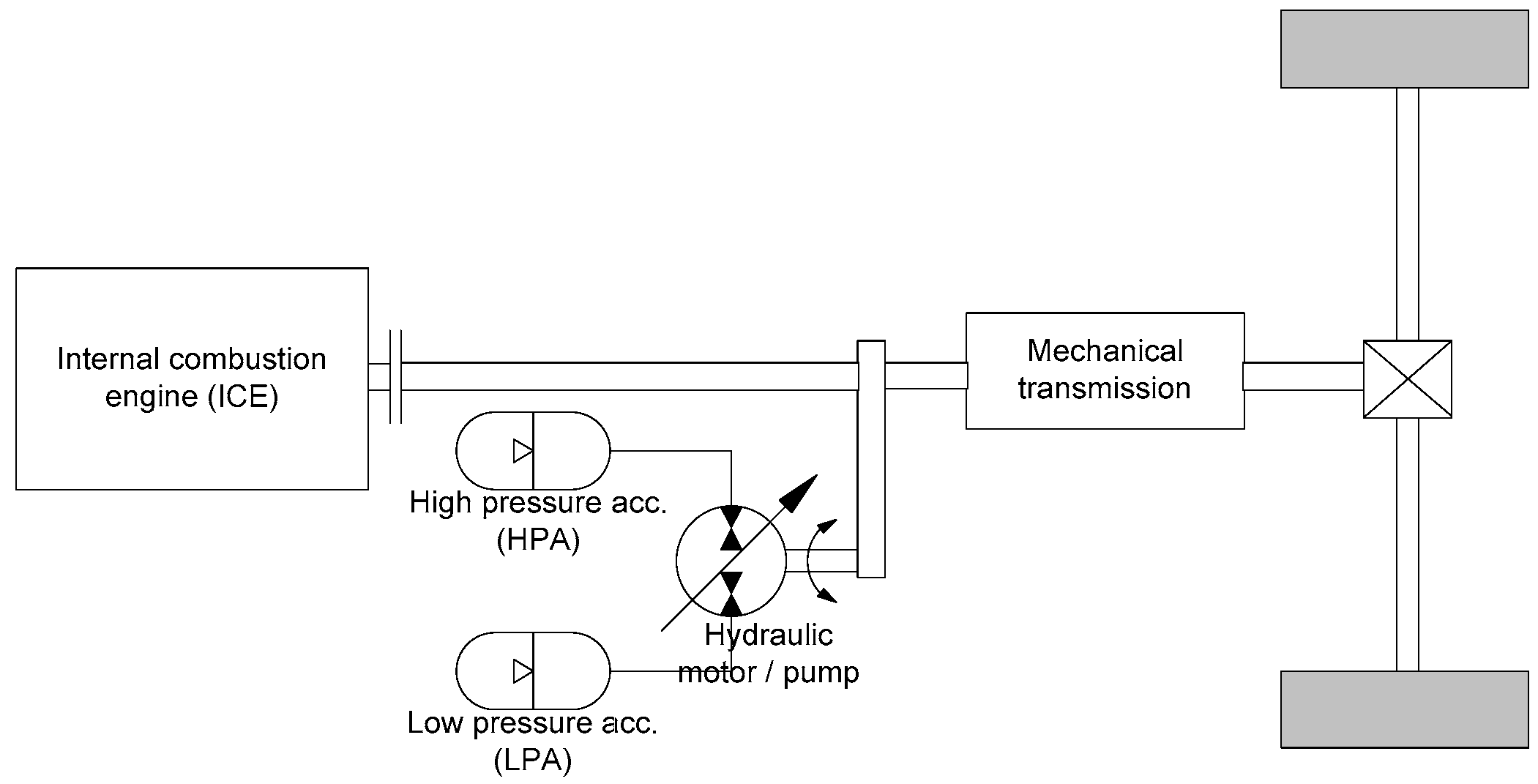
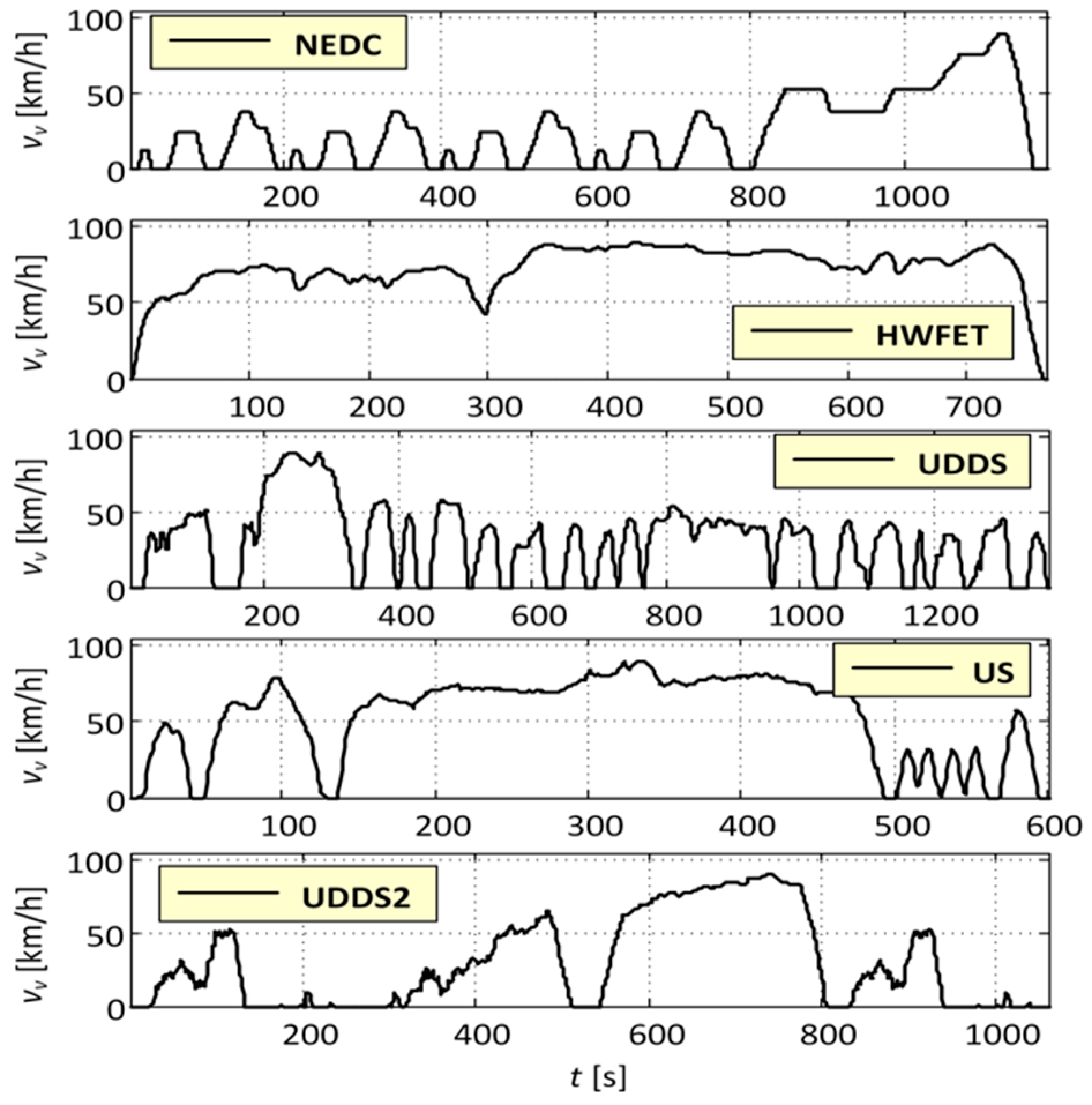
• Expanding the conventional drive with a hydraulic part that includes a hydraulic motor/pump unit and a hydro-pneumatic accumulator in a parallel configuration can reduce fuel consumption by 5% to 30% depending on the driving cycle characteristics (Table 4). More dynamic cycles that have a larger number of “stop-and-go” events score greater reduction (HWFET 4.6%, US 15.8%, UDDS2 18.3%, NEDC 19.6%, UDDS 29.8 %).
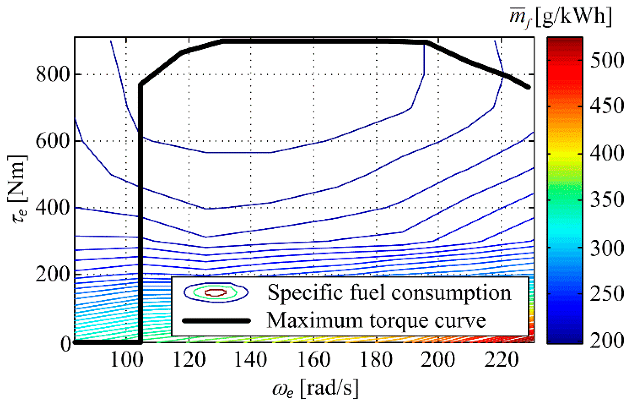
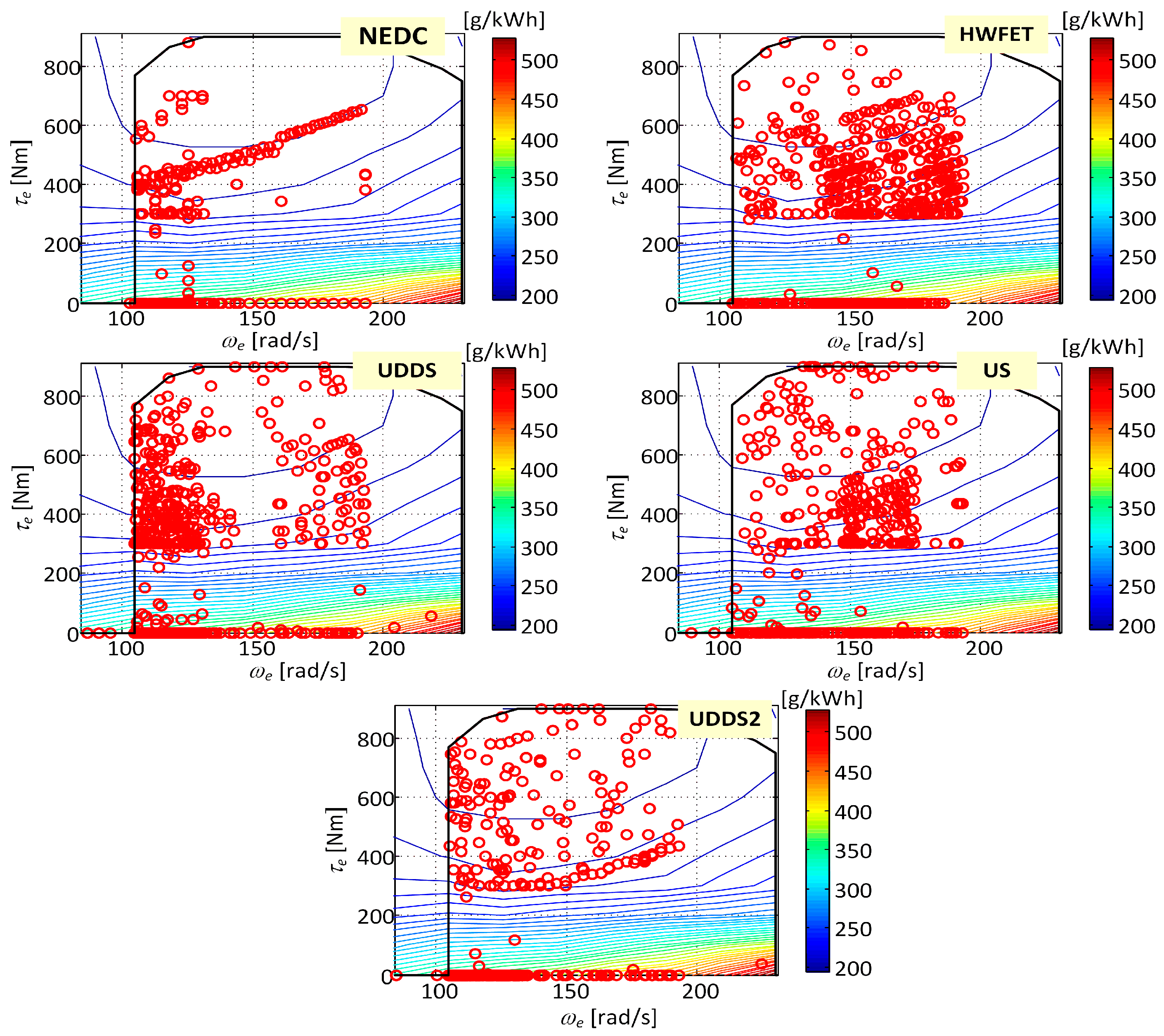
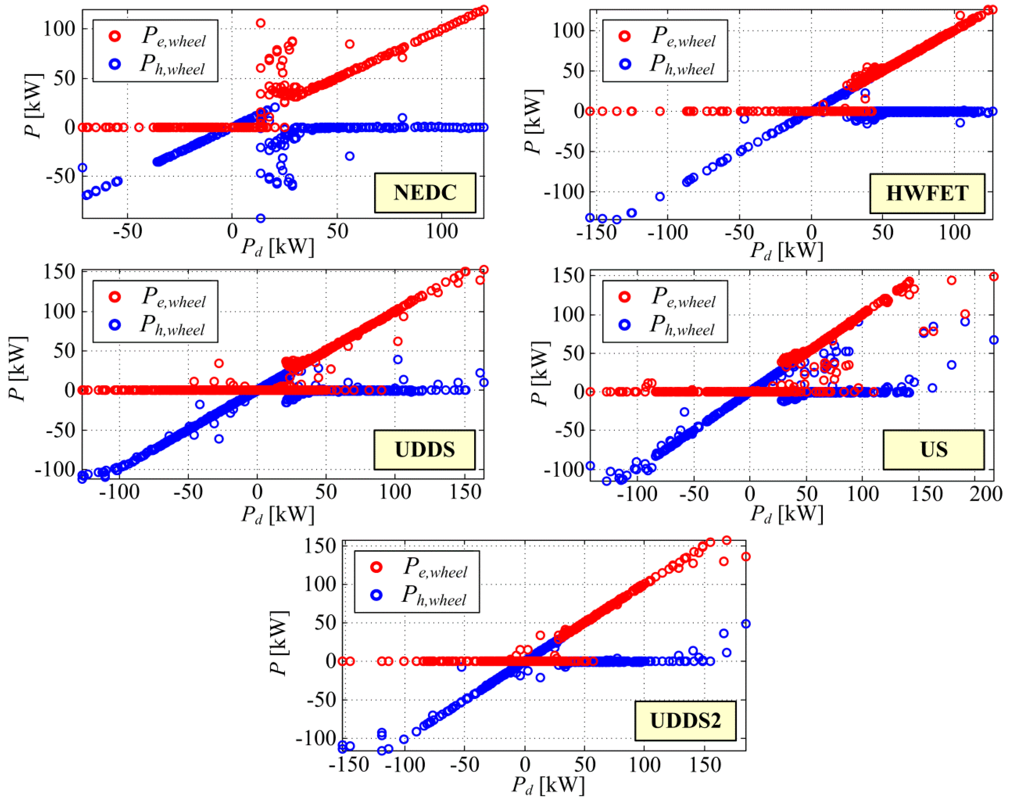
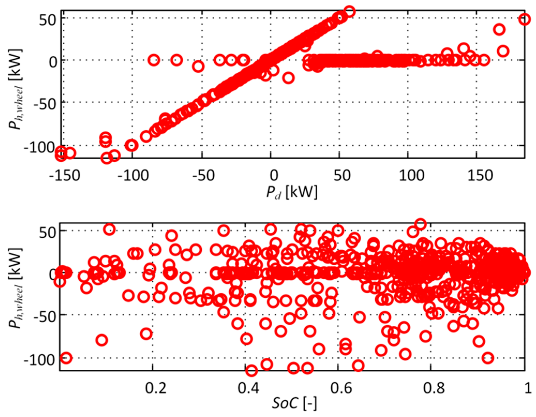
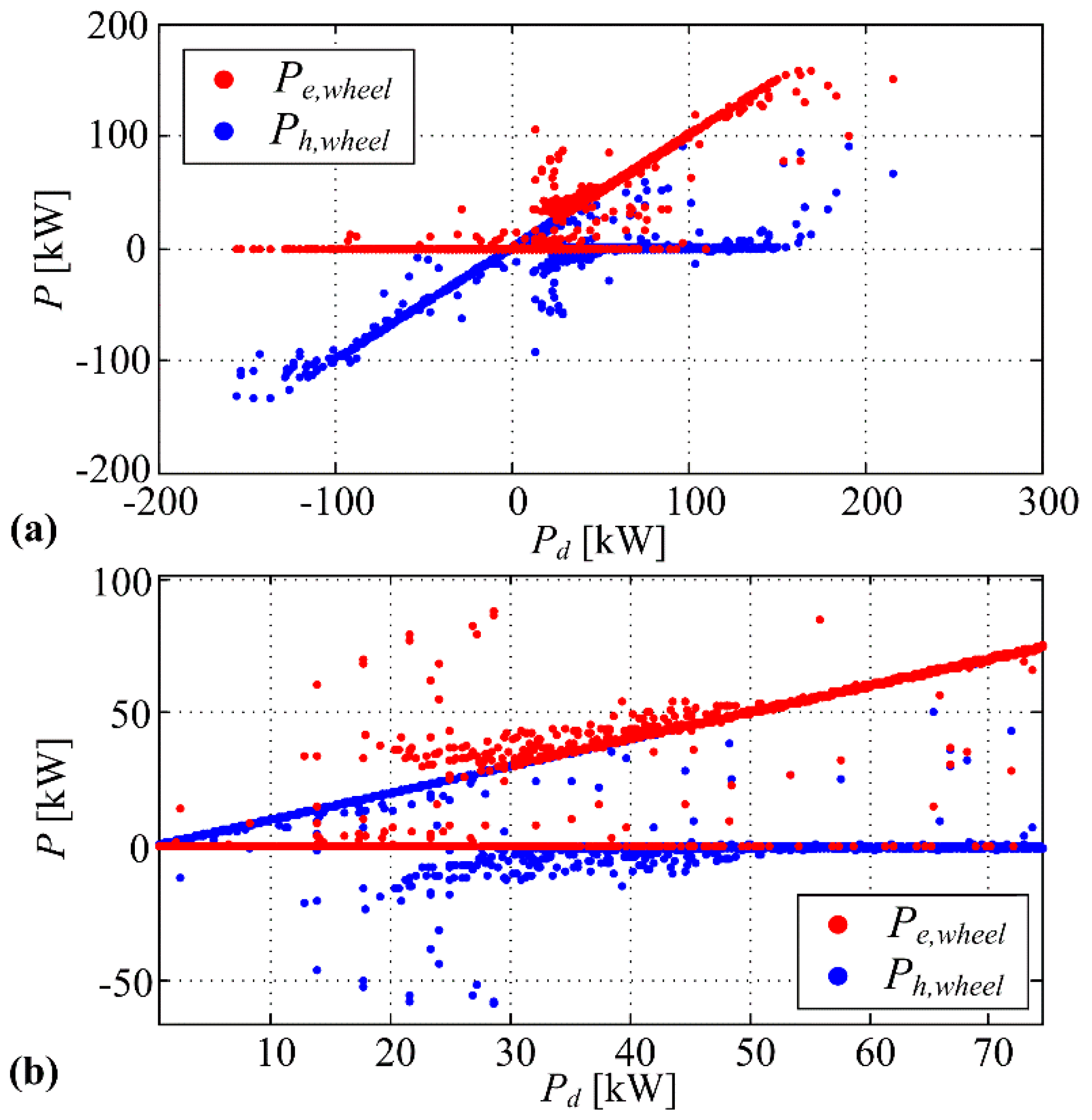
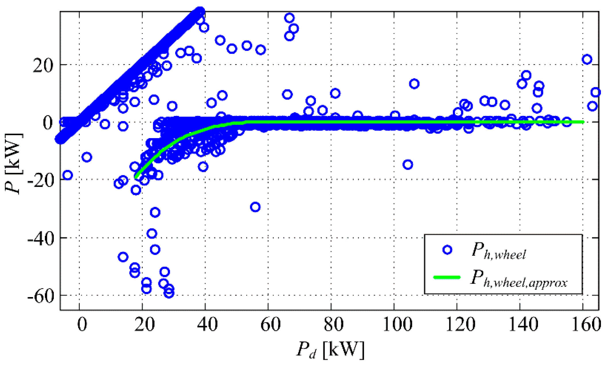
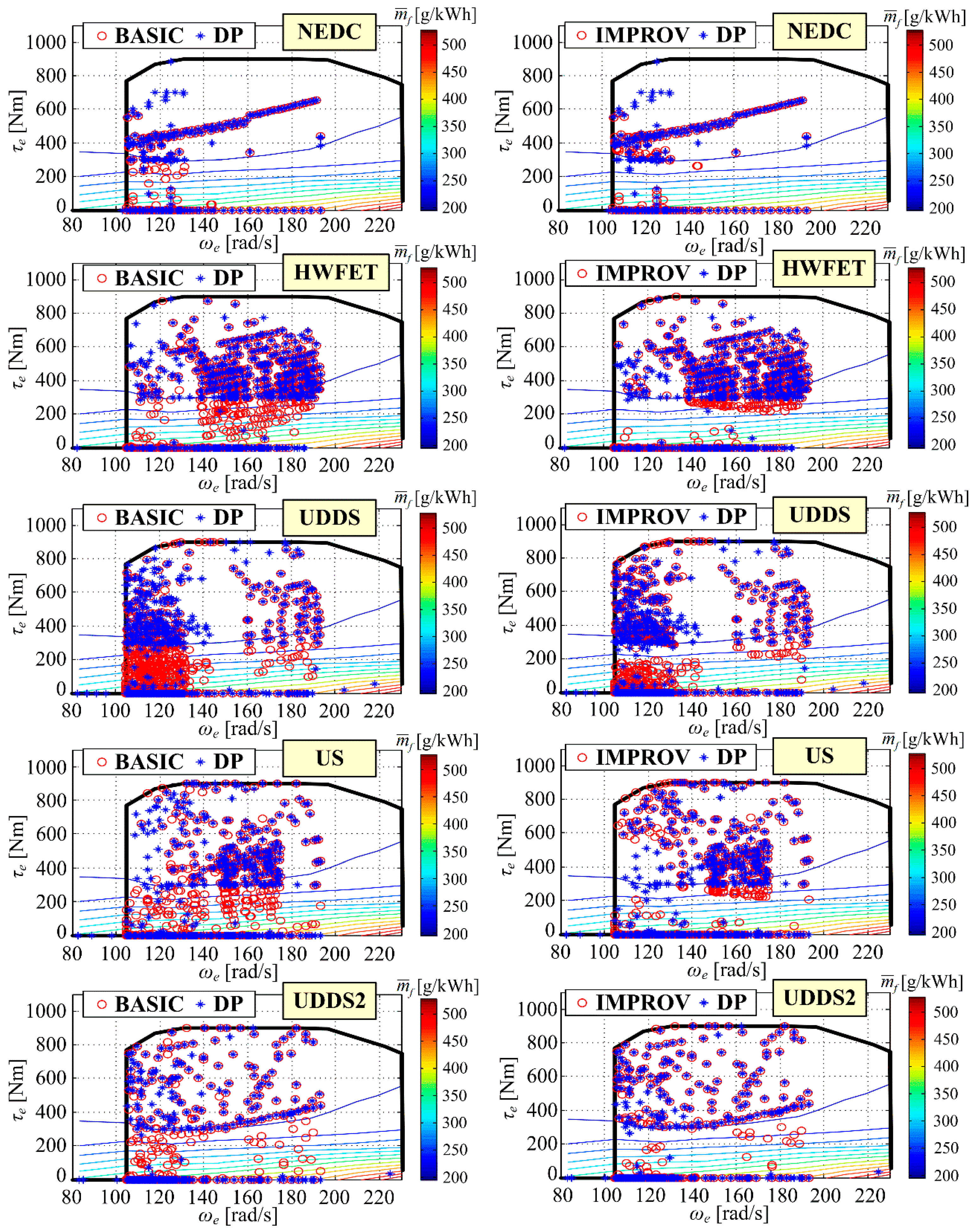
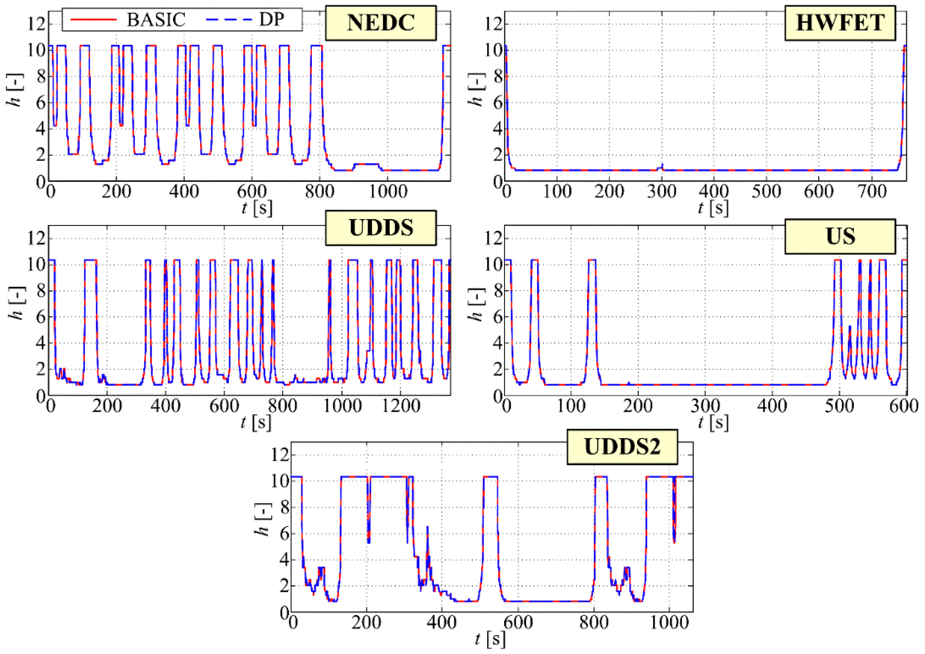
• The main characteristics that can be observed in the optimum DP results are: (i) consistent avoidance of ICE operating range between 0 and 300 Nm where the specific fuel consumption is quite large (Figure 7); (ii) SoC is trying to keep at a relatively high values to reduce losses in fluid flow (Figure 12 and Equations (7), (8) and (10)); (iii) For driver requirements for power P_d < 20 kW hydraulic motor delivers power and ICE is off; for power P_d > 50 kW ICE delivers power and hydraulic motor is off; and in the range between (20 kW < P_d < 50 kW) sometimes the driver’s demand meets the hydraulic motor and sometimes ICE which in that case gives a little more power than required in order to supplement the accumulator (Figure 10b).
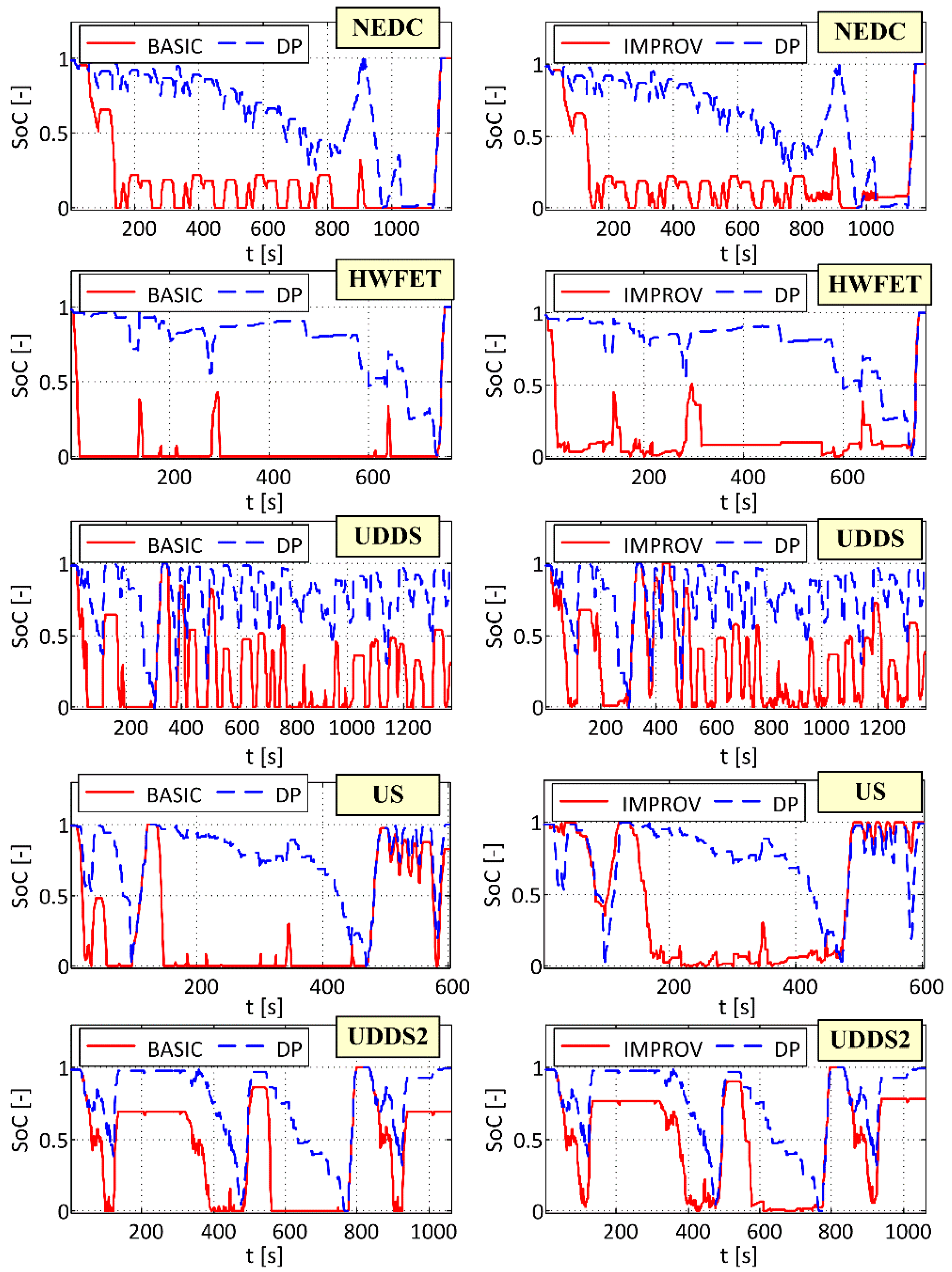
• The Basic (BASIC) and Improved (IMPROV) causal management strategies approach DP fuel consumption to 1–9% (NEDC + 4.6%, HWFET + 1.2%, UDDS + 8.6%, US 2.5%, UDDS2 + 0.9%) or to 1–7% (NEDC + 4.3%, HWFET +0.9%, UDDS + 6.5%, US + 7.0%, UDDS2 + 1.1%), respectively. That can be considered to be rather favourable respected that causal management strategies lack of “knowledge” of the whole cycle as opposed to DP optimization (Table 4).
• IMPROV management strategy has achieved a more similar distribution of ICE operating points as DP optimization. However, this did not result in a consistent reduction of fuel consumption compared to BASIC strategy for all cycles. The deviation from the minimum fuel consumption for both strategies (BASIC and IMPROV) can be explained essentially with the difference of BASIC and IMPROV SoC trajectories from the optimal DP SoC trajectories. If the SoC is “compulsory” held at higher values with lower losses, the potential for recovery of regenerative braking energy would be significantly reduced. Therefore, for further fuel consumption reduction using the causal management strategy, it is necessary to predict the driving cycle from which the optimal trajectory of SoC will be further estimated.

The proposed methodology for testing HHV using DP optimization can be improved by more accurate mathematical modelling, for example with a description of the gas state with the more realistic Benedict-Web-Rubin equation instead of the ideal gas equation, or with introduction of gas temperature as an additional state variable, or possibly with addition of the efficiency model of the hydraulic part. The implementation of DP algorithm in C would significantly accelerate the optimization process.

The suggestion of research activities on this topic in the future could be following:

• Predicting the driving cycle future based on the past cycle, calculating the optimal SoC trajectories for the anticipated driving cycle profile and applying the model predictive control (MPC),
• Considering Equivalent Consumption Management Strategy (ECMS) for HHV,
• Extending the existing management strategy with additional rules for example introducing different ICE deployment /exclusion thresholds and optimizing the same for different driving cycles,
• An analysis of DP optimization algorithm robustness to different changes in the model parameters values,
• The use of stochastic dynamic programming (SDP) for control which is possible, unlike the DP, to be implemented in a causal form, which has the advantage to “catch” trends in driving cycles in optimal way,
• Optimizing the HHV drive components dimensions using Willans descriptions of drive components,
• Identification and analysis of the statistical parameters of the driving cycles which are most dependent on the reduction of fuel consumption of HHV compared to CV. In this way, it is possible to examine what kind of driving cycles or applications it is profitable to apply hybridization.

7. Conclusions

The optimization of control variables and design of management strategy for a hybrid hydraulic vehicle in parallel configuration is a topic of the paper. The benefits of hybridization using hydraulics are analysed on the example of delivery truck. Its conventional drive using only ICE from the previous research is taken as a starting base and benchmark for comparison. Optimization of control variables is carried out using DP algorithm to gain insight into optimum operation of the driveline and minimum possible fuel consumption for five different driving cycles. Two rule based management strategies are given and compared. A simple causal management strategy was developed based on simple rules aimed at maximizing the utilization of regenerative braking energy. This basic strategy has been extended to certain rules that have been gained by insights into the optimum DP results, which, apart from the maximum utilization of regenerative braking energy, are to avoid the ICE operating range between 0 and 300 Nm, which is consistently present in DP results for different driving cycles. Hybrid driveline can reduce fuel consumption from 5% to 30% depending on the driving cycle. The main characteristics that can be observed in the optimum DP results are consistent avoidance of ICE operating range between 0 and 300 Nm where the specific fuel consumption is quite large and SoC is trying to keep at relatively high values to reduce losses in fluid flow.

Improvements of results could be achieved mainly through the upgrading of the mathematical model and applying the model predictive control (MPC). Some more suggestions for additional research on this topic are given in the previous Discussion section.

References

1. Hu, H.; Smaling, R.; Baseley, S.J. Advanced Hybrid Powertrains for Commercial Vehicles; SAE International: Warrendale, PA, USA, 2012; ISBN 978-0-7680-3359-5. [Google Scholar]
2. Guzella, L.; Sciarretta, A. Control of hybrid electric vehicles. IEEE Control Syst. 2007, 27, 60–70. [Google Scholar]
3. Guzella, L.; Sciarretta, A. Vehicle Propulsion Systems: Introduction to Modeling and Optimization; Springer: Berlin, Germany, 2013; ISBN 978-3-642-35913-2. [Google Scholar]
4. Zhao, K.; Liang, Z.; Huang, Y.; Wang, H.; Khajepour, A.; Zhen, Y. Research on a Novel Hydraulic/Electric Synergy Bus. Energies 2018, 11, 34. [Google Scholar] [CrossRef]
5. Filipi, Z. Hydraulic and pneumatic hybrid powertrains for improved fuel economy in vehicles. In Alternative Fuels and Advanced Vehicle Technologies for Improved Environmental Performance: Towards Zero Carbon Transportation; Woodhead Publishing Limited: Sawston, UK, 2014; pp. 505–540. [Google Scholar]
6. Škugor, B.; Cipek, M.; Deur, J. Control Variables Optimization and Feedback Control Strategy Design for the Blended Operating Mode of an Extended Range Electric Vehicle. SAE Int. J. Altern. Powertrain. SAE Pap. 2014, 3, 152–162. [Google Scholar] [CrossRef]
7. Škugor, B.; Deur, J.; Cipek, M.; Pavković, D. Design of a Power-split Hybrid Electric Vehicle Control System Utilizing a Rule-based Controller and an Equivalent Consumption Minimization Strategy. Proc. Inst. Mech. Eng. Part D J. Automob. Eng. 2014, 228, 631–648. [Google Scholar] [CrossRef]
8. Mustardo, C.; Rizzoni, G.; Guezennec, Y.; Staccia, B. A-ECMS: An adaptive algorithm for hybrid electric vehicle energy management. Eur. J. Control 2005, 11, 509–524. [Google Scholar] [CrossRef]
9. Onori, S.; Serrao, L. On adaptive-ECMS strategies for hybrid electric vehicles. In Proceedings of the International Scientific Conference on Hybrid and Electric Vehicles, Rueil-Malmaison, France, 6–7 December 2011. [Google Scholar]
10. Qin, F.; Xu, G.; Hu, Y.; Xu, K.; Li, W. Stochastic Optimal Control of Parallel Hybrid Electric Vehicles. Energies 2017, 10, 214. [Google Scholar] [CrossRef]
11. Xu, G.; Li, W.; Xu, K.; Song, Z. An Intelligent Regenerative Braking Strategy for Electric Vehicles. Energies 2011, 4, 1461–1477. [Google Scholar] [CrossRef] [Green Version]
12. Samadani, E.; Farhad, S.; Panchal, S.; Fraser, R.; Fowler, M. Modeling and Evaluation of Li-Ion Battery Performance Based on the Electric Vehicle Field Tests; SAE International: Warrendale, PA, USA, 2014. [Google Scholar] [CrossRef]
13. Karbaschian, M.A.; Söffker, D. Review and Comparison of Power Management Approaches for Hybrid Vehicles with Focus on Hydraulic Drives. Energies 2014, 7, 3512–3536. [Google Scholar] [CrossRef] [Green Version]
14. Kim, H.; Wi, J.; Yoo, J.; Son, H.; Park, C.; Kim, H. A Study on the Fuel Economy Potential of Parallel and Power Split Type Hybrid Electric Vehicles. Energies 2018, 11, 2103. [Google Scholar] [CrossRef]
15. Cipek, M.; Škugor, B.; Deur, J. Comparative Analysis of Conventional and Electric Delivery Vehicles Based on Realistic Driving Cycles. In Proceedings of the EEVC European Electric Vehicle Congress (EEVC-2014), Brussels, Belgium, 2–5 December 2014. [Google Scholar]
16. Mance, M. Mathematical Modelling of Hybrid Hydraulic Vehicle. Bachelor’s Thesis, University of Zagreb, Zagreb, Croatia, 4 March 2014. (In Croatian). [Google Scholar]
17. How Parallel Hydraulic Hybrid Vehicles Work. Available online: https://archive.epa.gov/otaq/technology/web/html/how-it-works-parallel.html (accessed on 12 October 2018).
18. Pfeffer, A.; Glück, T.; Kemmetmüller, W.; Kugi, A. State of Charge Estimator Design for a Gas Charged Hydraulic Accumulator. J. Dyn. Syst. Meas. Control 2015, 137. [Google Scholar] [CrossRef]
19. Lemofouet, S. Investigation and Optimization of Hybrid Electricity Storage Systems Based on Compressed Air and Supercapacitors. Ph.D. Thesis, Ecole Polytechnique Federale de Lausanne, Lausanne, Switzerland, 20 October 2006. [Google Scholar]
20. Perković, V. Short-time energy storage using hydro-pneumatic accumulators. Master’s Thesis, University of Zagreb, Zagreb, Croatia, 15 December 2011. (In Croatian). [Google Scholar]
21. Petrić, J. Modeling of hydro-pneumatic energy storage system. In Proceedings of the 8th EUROSIM Congress on Modelling and Simulation, Cardiff, UK, 10–13 September 2013. [Google Scholar]
22. Pfeffer, A.; Glück, T.; Kemmetmüller, W.; Kugi, A. Mathematical modelling of a hydraulic accumulator for hydraulic hybrid drives. Math. Comput. Model. Dyn. Syst. 2016, 22, 397–411. [Google Scholar] [CrossRef]
23. Bellman, R.E.; Dreyfus, S.E. Applied Dynamic Programming; Princeton University Press: Princeton, NJ, USA, 1962; ISBN 978-0691625423. [Google Scholar]
24. Giakoumis, E.G. Driving and Engine Cycles; Springer International Publishing AG: Cham, Switzerland, 2017; ISBN 978-3-319-49033-5. [Google Scholar]
25. 2016 Chevrolet Volt Battery System. Available online: https://media.gm.com/content/dam/Media/microsites/product/Volt_2016/doc/VOLT_BATTERY.pdf (accessed on 12 October 2018).
Figure 1. Delivery truck MAN TGM 15.240.
Energies 11 02838 g001
Figure 2. Block diagram of quasi-static model of conventional driveline. ICE: internal combustion engine.
Energies 11 02838 g002
Figure 3. Specific consumption map and maximum torque curve of ICE.
Energies 11 02838 g003
Figure 4. Hybrid hydraulic vehicle (HHV) in parallel configuration.
Energies 11 02838 g004
Figure 5. Block diagram of quasi-static model of hydraulic hybrid driveline in parallel configuration.
Energies 11 02838 g005
Figure 6. Certification driving cycles [24].
Energies 11 02838 g006
Figure 7. Optimum operating points of ICE obtained by DP optimization for different driving cycles.
Energies 11 02838 g007
Figure 8. Optimum wheel power from ICE (Pe,wheel) and hydraulic motor/pump (Ph,wheel).
Energies 11 02838 g008
Figure 9. Dependence of the optimum power of the hydraulic motor supplied to the wheels Ph,wheel on the required power Pd and SoC for each driving cycle.
Energies 11 02838 g009
Figure 10. Optimum power for all cycles: (a) optimum ICE Pe,wheel and hydraulic motor power Ph,wheel; (b) detail from (a).
Energies 11 02838 g010
Figure 11. Detail from Figure 10, hydraulic motor power Ph,wheel and approximation curve Ph,wheel,approx.
Energies 11 02838 g011
Figure 12. SoC trajectories of BASIC and IMPROV management strategies presented parallel to optimum SoC trajectories obtained by DP optimization for different driving cycles.
Energies 11 02838 g012
Figure 13. ICE operating points of BASIC and IMPROV control strategies presented parallel to optimum operating points obtained by DP optimization for different driving cycles.
Energies 11 02838 g013
Figure 14. Gear ratios h of BASIC management strategy presented parallel to optimum gear ratios obtained by DP optimization for different driving cycles.
Energies 11 02838 g014