Hierarchical Energy Management for the MultiEnergy Carriers System with Different Interest Bodies

Abstract

Multi-energy carriers system (MECS), in which diverse energy carriers and different energy systems interact together, has drawn the interest of many researchers in recent years. However, the optimal economic operational model of the MECS is a nonlinear, multi-variable, and multi-period problem, of which it is difficult to find the solution because several different energy flows are integrated in the system. To this end, three interest bodies in the MECS were investigated, which included the energy provider, the energy facilitator, and the energy consumer, and a hierarchical optimal economic operation strategy was then presented. A hybrid optimization strategy combining the swarm intelligence algorithm and interior point method was developed taking advantage of the merits of each method. Case studies were conducted to verify the effectiveness of the proposed hierarchical optimal economic operation strategy, whereby demonstrating that the proposed strategy can achieve rational energy allocation and decrease the energy cost in the MECS compared with traditional energy systems.

1. Introduction

Energy has become the cornerstone of human survival and development. How to reasonably allocate energy and cut down system costs on the premise of meeting energy needs has attracted the attention of many scholars in the world [1]. Hereinto, it is particularly important to change the existing energy systems which are designed to operate separately, and to synthetically plan and operate various energy systems together to boost the synergical effect throughout the total energy systems. Therefore, some coupled energy systems, such as the integrated energy system (IES) [2], the multiple-energy carriers system (MECS) [3], and multi-energy systems (MES) [4], have been investigated quite intensively in recent years. The essential characteristic of these energy systems is the interaction of diverse forms of energy, such as electricity, natural gas, heat, cooling, and so on. Several coupling components, for instance, combined cooling, heat and power unit (CCHP), gas boiler, electric boiler, wind turbine, photovoltaic cell, fuel cell, plug-in hybrid electric vehicles or other devices, have been taken into account to accomplish the production, delivery and consumption of energy resources jointly [5,6]. Furthermore, the energy storage system should be integrated into the energy system in order to increase energy efficiency and decrease operating cost.

To model the MECS, the concept of the energy hub, which is regarded as an interface between coupling components and loads, was proposed in [7]. According to [8], the energy hub is a promising tool for integrated management in MES due to its four main functions: production, conversion, storage, and consumption. With these four features, the energy hub could be employed in the design or planning stage and operation or scheduling stage. In [9], the energy hub model is employed as a system simulation tool in the concept stage of a building design which can avoid ranking a series of different system configurations. According to [10], a framework is presented for optimal planning of energy hubs considering the physical constraints of the electricity and natural gas networks. In [11], suitable operation modes for the energy hub are presented and the roles of the energy hub in electricity price uncertainty are investigated. In addition, an optimization program is proposed to schedule the renewable distributed energy resources to achieve the load management for minimizing the customer payment cost [12]. Moreover, the energy hub model could be employed in different regions. A general optimal industrial load management model is integrated into the energy hub management system in [13]. A residential energy hub model is investigated and, for augmenting the operational flexibility, an inclusive demand response is considered, which contains load shifting, load curtailing, and flexible thermal load management [14]. In [15], decentralized energy systems are integrated based on the energy hub approach at the neighborhood scale, and the energy-autonomy, as well as the economic and ecological performance are evaluated simultaneously.

However, most of these studies mainly concentrate on the modeling of MECS, and as well the model of transmission networks, such as electricity, natural gas, and district heating (DH) networks, should be considered adequately. A general multiple energy carrier power flow model was developed based on nodal power balance, and line losses were calculated as polynomial functions of the corresponding power flow [16]. The nonlinear model of the gas network was formulated in detail containing gas well, gas pipeline, gas compressor, gas loads, and so on [17,18,19]. In [20], a natural gas network system was incorporated in IES, and the gas shift matrix, similar to the generation shift factor in DC power flow model, was formulated to linearize the pipeline flow equation so that the computational efficiency was improved. In [21], a power distribution system (PDS) and a district heating system (DHS) were regarded as a whole to build the steady-state model of hybrid energy flow. To investigate the performance of electricity and heat networks, models of combined electricity and district heating networks were established; in addition, decomposed and integrated electrical-hydraulic-thermal calculation methods were proposed [22].

Extensive researches have been conducted on the optimal operation for MECS, which is modeled based on the concept of the energy hub. Some researchers proposed a mixed integer linear programming (MILP) problem, which was solved by the CPLEX solver in the General Algebraic Modeling System (GAMS) considering deterministic and stochastic formulations [23,24], the thermal energy market [25], and the demand response program [26]. Although the commercial solver represents high effectiveness for some simple optimization problems, evolutionary techniques might perform better in finding the optimal solution for such high-dimensional, non-smooth, non-linear, and multi-period problems. A complex energy network containing 39 energy hubs with 29 structures were solved by self-adaptive learning with the time-varying acceleration coefficient-gravitational search algorithm (SAL-TVAC-GSA) [27]. A modified teaching-learning based optimization (MTLBO) algorithm was carried out for the multi-objective optimal power flow problem for the IEEE 30-bus and 57-bus systems, which considers a self-adapting wavelet mutation strategy for the modified phase, and merges with fuzzy clustering for better population selection [28]. Furthermore, this algorithm was employed to solve the operation management and optimal power flow problem in MECS [29,30]. To acquire the optimal solution for a whole day, a multi-agent genetic algorithm (MAGA) was proposed for the online economic dispatch problem. The MAGA is a robust optimization technique and has the characteristic of finding the global optimal solution, where the economic dispatch problem could be divided into 24 sub-problems without an energy storage system [31,32].

However, when energy storage systems are utilized, the dispatch results at the present time are affected by the results in previous intervals. To cope with the dynamic characteristics resulting from the storage systems in MECS, a model predictive control strategy was proposed in [33]. A multi-objective optimal energy management model was developed and solved by the non-dominated sorting genetic algorithm II (NSGA II) based on a system which contains integrated electrical and natural gas networks [34]. However, in most of these studies, the optimal operation model was built and solved without considering the system structure and the interest bodies in the MECS. Therefore, a hierarchical optimal operation strategy is proposed in this paper considering different interest bodies due to the MECS structure. The major innovation of this paper can be summarized into the following two aspects.

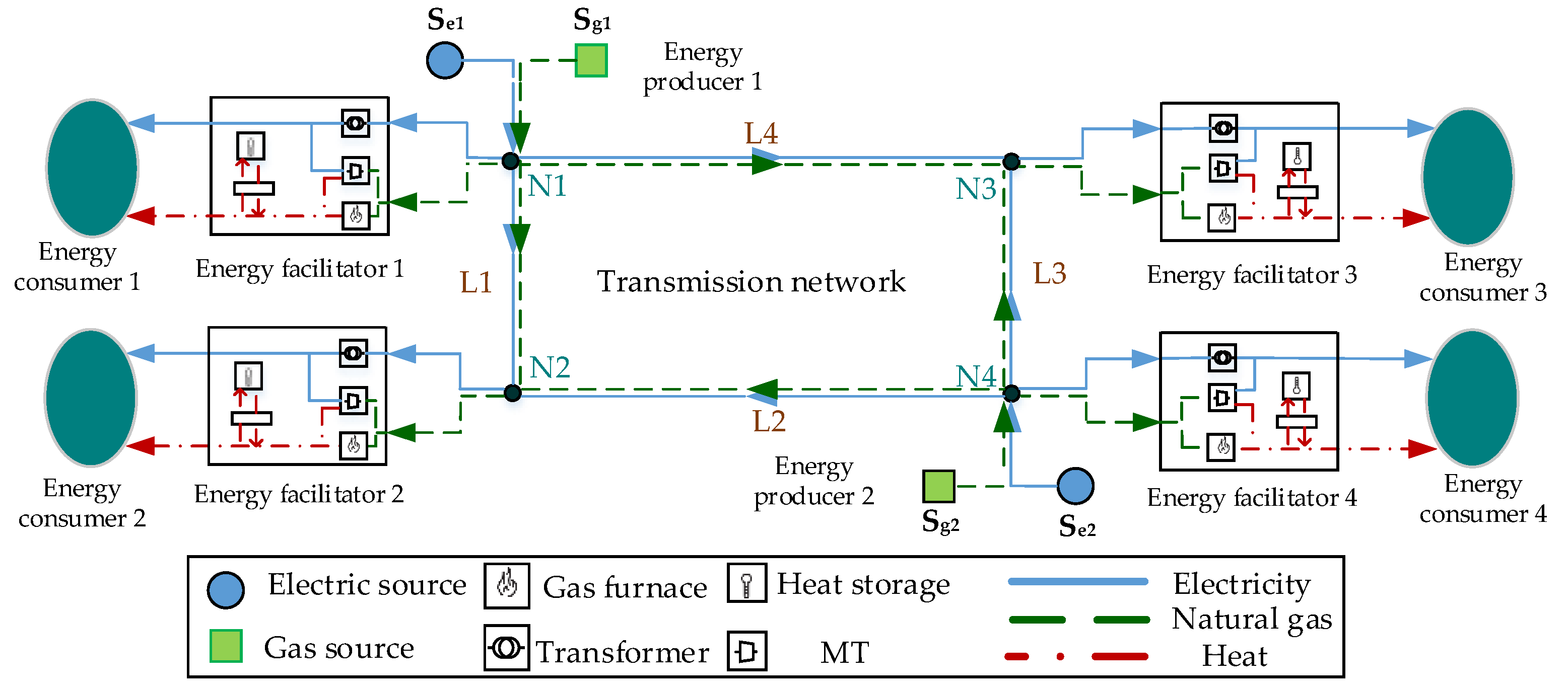
• Three interest bodies are analyzed in this paper, which are energy provider, energy facilitator, and energy consumer. The energy facilitator model is conducted based on the energy hub concept. Transmission network models between the energy provider and energy facilitator are provided.
• A hierarchical optimal economic operation strategy is formulated based on the above three different interest bodies in the MECS. Two optimization problems with the aims of minimizing the cost of the energy facilitator and that of the energy provider are formulated and solved.

The rest of this paper is organized as follows. In Section 2, transmission network models between the energy provider and energy facilitator are developed, and in addition, an energy facilitator model is developed. A hierarchical energy management strategy is developed in Section 3. Case studies and results are discussed in Section 4. Finally, the conclusions of this paper are collated in Section 5.

2. Modeling of MECS

The aim of MECS is to achieve the purposes of reducing the system operating cost, locally assimilating renewable energy, and enhancing systemic reliability on the premise of satisfying different types of energy demand on the customer side. The MECS is comprised of three main interest bodies in this paper, which are regarded as the energy provider, energy facilitator, and energy consumer, as shown in Figure 1. Various kinds of energy are transferred through different transmission networks from energy providers and then they are converted or stored by energy facilitators to meet the diverse energy needs of the energy consumers. To achieve the optimal economic operation, the modeling of MECS plays a fundamental role. This section attempts to acquire the mathematical formulations of the transmission network and energy facilitator in the MECS.

2.1. Transmission Network Model

Transmission network plays an important role in energy transfer between energy providers and energy facilitators in MECS. However, energy loss is an unavoidable phenomenon in this process, which can be considered in the transmission network model as shown in Figure 2.

Therefore, a general modeling approach for the transmission network is presented in this part [16]. The steady pipeline model is developed as follows [35]:

$$F_{\mathrm{MN},\mathsf{\alpha }}=-F_{\mathrm{NM},\mathsf{\alpha }}+\mathsf{\Delta }{F}_{\mathrm{MN},\mathsf{\alpha }}$$

(1)

where F_MN,α represents the α-th energy flow which leaves from node M to node N; ΔF_MN,α represents the energy losses when the α-th energy carrier flows from node M to node N. In this paper, α is electricity (e), natural gas (g) and heat (h).

According to [16], the energy losses on the pipeline can be approximated as a polynomial function of the corresponding energy flow which is shown as flows:

$$\mathsf{\Delta }{F}_{\mathrm{MN},\mathsf{\alpha }}={\displaystyle \sum _{k=1}^{K_{\mathsf{\alpha }}}{f}_{\mathrm{MN},\mathsf{\alpha }k}{\left|F_{\mathrm{MN},\mathsf{\alpha }}\right|}^{{}^k}}$$

(2)

where f_MN,αk is the loss coefficients, K_α is the maximum order which depends on the kind of energy carrier.

It is assumed that each energy facilitator on the transmission network is regarded as a node. Therefore, based on the Kirchhoff Law, for the transmission network which has n load nodes, m source nodes, and k lines, the general mathematical model for the α-th energy carrier in the transmission network can be obtained as:

$${\mathit{P}}_{\mathsf{\alpha }}={\mathit{A}}_{\mathsf{\alpha }}{\mathit{F}}_{\mathsf{\alpha }}-{\mathit{A}}_{\mathit{L}\mathsf{\alpha }}\mathsf{\Delta }{\mathit{F}}_{\mathsf{\alpha }}+{\mathit{A}}_{\mathrm{s}\mathsf{\alpha }}{\mathit{S}}_{\mathsf{\alpha }}$$

(3)

where P_α is the α-th energy for energy facilitators with n × 1 dimensions; A_α is called the line connection matrix with n × k dimensions, where the value set of all elements is {0, +1, −1}; F_α is the α-th energy flow in each line with k × 1 dimensions; A_Lα is the energy loss connection matrix with n × k dimensions; ΔF_α is the energy loss in each line with k × 1 dimensions; A_Sα is defined as the source connected matrix with n × m dimensions; and S_α is the source output with m × 1 dimensions.

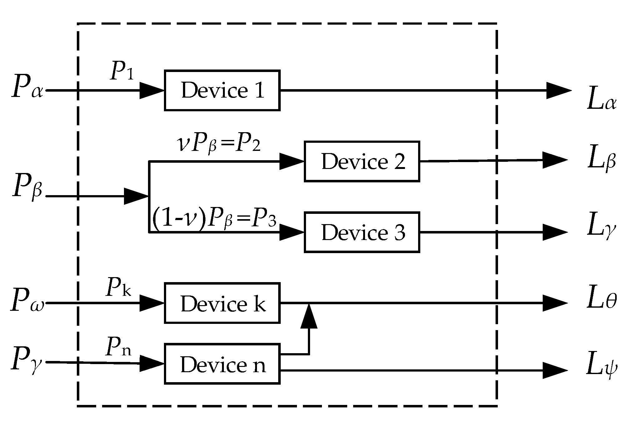
2.2. Energy Facilitator Model

In this part, the energy facilitator is modeled by the concept of the energy hub which has been applied widely in multiple energy carrier systems. The energy providers input various types of energy, such as electricity, heat, natural gas, and so on, to the energy facilitators which, combined with various internal energy treatment devices, realize the joint transfer and storing of energy and other functions to fulfill the diverse kinds of energy needs of the energy consumer. There are two main kinds of devices which the energy facilitator possesses, namely energy storage devices and energy conversion devices. Energy storage devices, such as battery, gas storage facility, and heat storage device, can charge or discharge energy for adjusting the energy need based on the operation principle. Energy conversion devices can convert the energy into different types or just serve one kind of energy. For example, the microturbine (MT) can utilize natural gas for producing electricity and heat, while the transformer’s input and output are both electricity. Energy conversion efficiency is utilized in modeling devices with energy losses present in the energy storing and conversion processes.

2.2.1. Storage Device Model

The storage devices, as shown in Figure 3, include an ideal storage and an interface unit linked with pipelines [35]. The storage device has energy charging and discharging functions, but only one function can be utilized in one interval.

Its mathematical model is expressed as follows [35]:

$$\{\begin{array}{l}\overline{Q}=eQ\\ e=\{\begin{array}{ll}{e}_{}^{+}& \left(\mathrm{charging}\right)\\ 1/e_{}^{-}& \left(\mathrm{discharging}\right)\end{array}\end{array}$$

(4)

where e⁺ and e⁻ represent the interface efficiency in different functions. When energy flows from the pipeline to the storage device, e is equal to e⁺. Otherwise, e is equal to 1/e⁻. In order to describe the operation mode of the storage device more directly, this paper introduces the storage factor s. The relationship between s and quantity of energy charging or discharging from the storage device is expressed as follows:

$$\overline{Q}=s{E}_{\max }$$

(5)

where $\overline{Q}$ is the charging or discharging quantity of the storage device, and E_max is the upper storage capacity limit of the storage device. From this formula, it is easy to see a linear relationship between the energy variation of the storage device and the storage factor. So when s is positive, this means the storage device is reserving; when s is negative, this indicates the device is releasing. Therefore, the energy of the storage device at time t is:

$$E(t)=E(t-1)+\overline{Q}(t)-E_{\mathrm{loss}}\left(t\right)$$

(6)

where E(t) is the energy quantity in the storage device at time t; E_loss(t) is the energy loss of this device at interval t.

2.2.2. Conversion Device Model

As noted earlier, steady energy converting efficiency is used to describe the mathematical model of energy conversion devices. An energy hub contains many conversion devices to realize energy conversion and transfer, as depicted in Figure 4.

The dispatch factor ν is introduced to describe the energy distribution for more than one device consuming the same kind of energy simultaneously [31]. The dispatch factors describe how the energy carrier is distributed between each conversion device, as shown in Figure 4. The mathematical model of the conversion device is expressed as follows:

$$\underset{L}{\underbrace{\left[\begin{array}{l}{L}_{\mathsf{\alpha }}\\ L_{\mathsf{\beta }}\\ .\\ .\\ .\\ L_{\mathsf{\psi }}\end{array}\right]}}=\underset{C}{\underbrace{\left[\begin{array}{cccc}\begin{array}{l}{c}_{\mathsf{\alpha },\mathsf{\alpha }}\\ c_{\mathsf{\beta },\mathsf{\alpha }}\\ .\\ .\\ .\\ c_{\mathsf{\psi },\mathsf{\alpha }}\end{array}& \begin{array}{l}{c}_{\mathsf{\alpha },\mathsf{\beta }}\\ c_{\mathsf{\beta },\mathsf{\beta }}\\ .\\ .\\ .\\ c_{\mathsf{\psi },\mathsf{\beta }}\end{array}& \begin{array}{l}\dots \\ \dots \\ \\ \\ \\ \dots \end{array}& \begin{array}{l}{c}_{\mathsf{\alpha },\mathsf{\omega }}\\ c_{\mathsf{\beta },\mathsf{\omega }}\\ .\\ .\\ .\\ c_{\mathsf{\psi },\mathsf{\omega }}\end{array}\end{array}\right]}}\underset{P}{\underbrace{\left[\begin{array}{l}{P}_{\mathsf{\alpha }}\\ P_{\mathsf{\beta }}\\ .\\ .\\ .\\ P_{\mathsf{\omega }}\end{array}\right]}}$$

(7)

where L_α denotes the α-th load for the energy consumer; P_β represents the β-th energy supply from the transmission network; c_α,β is determined by the steady-state energy conversion efficiency and dispatch factor ν for the β-th energy carrier, and C is called the coupling matrix.

2.2.3. Energy Hub Model

Based on the energy storage device model and energy conversion device model, the mathematical energy hub model is described as follows:

$$\mathit{L}=\mathit{C}\mathit{P}-\mathit{S}{\mathit{E}}_{\mathit{max}}$$

(8)

where S is the storage matrix, E_max is the upper storage capacity vector.

3. Hierarchical Energy Management Strategy

As proposed earlier, the MECS is comprised of three parts, which are the energy providers, energy facilitators, and energy consumers, as described in Figure 1. To coordinate the interests of these three parts, a hierarchical energy management strategy is presented in this section.

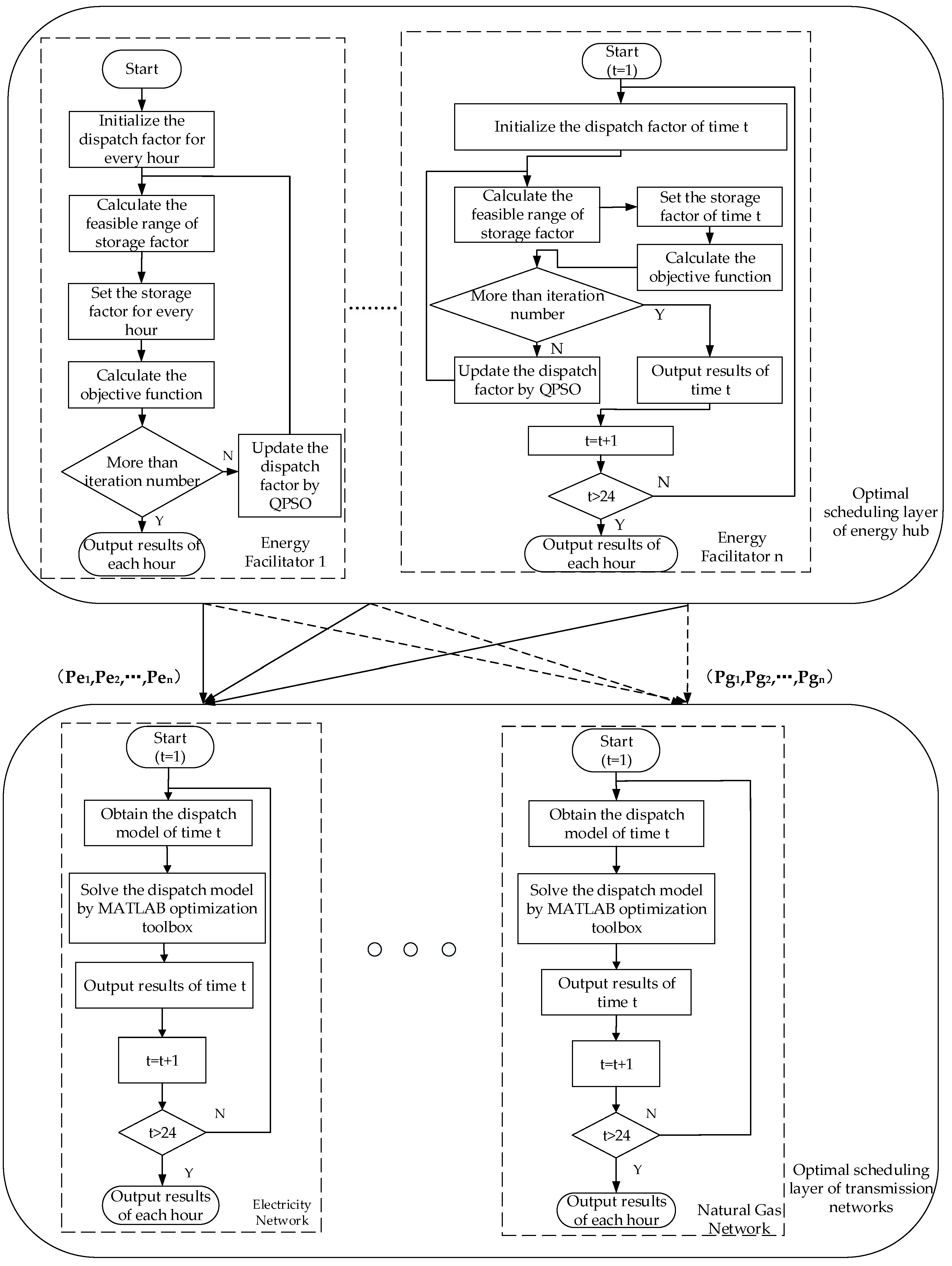
3.1. Hierarchical Economic Scheduling Framework

As illustrated in Figure 5, a hierarchical economic scheduling framework is proposed with two optimal blocks, which are the optimal scheduling layer of the energy hub and the optimal scheduling layer of the transmission network.

In the optimal scheduling layer of the energy hub, energy facilitators focus on determining the optimal energy distribution in each energy facilitator. Furthermore, after fixing the optimal dispatch strategy within each energy facilitator, the optimal scheduling layer of the transmission network is provided to arrange the energy supply of the energy providers for fulfilling the energy needs from the energy facilitators.

3.2. Optimal Economic Dispatch Model

Combined with the MECS model and the hierarchical optimal scheduling framework, the optimal economic dispatch model for each layer is formulated in this part. To illustrate the optimal economic dispatch model explicitly, an MECS model is considered in Figure 6, which has two energy providers, four energy facilitators, and four energy consumers.

3.2.1. Objective Function

For the optimal scheduling layer of the energy hub, the optimal scheduling aim in this paper is to spend the least amount of money on purchasing electric power and natural gas for 24 h of the day.

The objective function for each energy facilitator is described as:

$$\min {\displaystyle \sum _{t=1}^{24}\left[a_{\mathrm{e}}(t)P_{\mathrm{e}}(t)+a_{\mathrm{g}}(t)P_{\mathrm{g}}(t)\right]}$$

(9)

where a_e(t) is the electricity price at time t in MECS, and P_e(t) is the power needs of energy facilitator at time t; a_g(t) is the natural gas price at time t in MECS, and P_g(t) is the natural gas needs of the energy facilitator at time t.

In terms of the optimal scheduling layer of the transmission network, the aim of optimal scheduling is to minimize the losses in each transmission network on the premise of meeting the energy needs of energy facilitators, which means the minimum energy supply or minimum energy cost of the energy providers. The objective function of each transmission network is developed as:

$$\min {\displaystyle \sum _{t=1}^{24}{\displaystyle \sum _{i=1}^2{a}_{\mathsf{\alpha }}(t)S_{\mathsf{\alpha }\mathrm{i}}(t)}}$$

(10)

where S_αi(t) is the α-th energy supplied by the i-th energy provider at time t, a_α (t) is the α-th energy price at time t.

3.2.2. Equality Constraints

For the optimal scheduling layer of the energy hub, it is necessary to satisfy the equality constraints of Equation (8), that is, each energy facilitator should meet the energy balance of input and output. The equality constraints for an energy facilitator are shown as follows:

$$\left[\begin{array}{c}{L}_{\mathrm{e}}(t)\\ L_{\mathrm{h}}(t)+\frac{s(t)E_{\max ,\mathrm{h}}}{e_{\mathrm{h}}}\end{array}\right]=\left[\begin{array}{l}\begin{array}{cc}{\eta }_{\mathrm{ee}}^{\mathrm{T}}& \nu (t){\eta }_{\mathrm{ge}}^{\mathrm{MT}}\end{array}\\ \begin{array}{cc}0& \nu (t){\eta }_{\mathrm{gh}}^{\mathrm{MT}}+(1-\nu (t)){\eta }_{\mathrm{gh}}^{\mathrm{F}}\end{array}\end{array}\right]\left[\begin{array}{l}{P}_{\mathrm{e}}(t)\\ P_{\mathrm{g}}(t)\end{array}\right]$$

(11)

where L_e(t) and L_h(t) are respectively electricity and heat load, P_e(t) and P_g(t) are respectively electricity and gas supply, ${\mathsf{\eta }}_{\mathrm{ee}}^{\mathrm{T}}$ is the efficiency of transformer, ${\eta }_{\mathrm{ge}}^{\mathrm{MT}}$ is the electricity generating efficiency of MT, ${\eta }_{\mathrm{gh}}^{\mathrm{MT}}$ is the heat generating efficiency of MT, ${\eta }_{\mathrm{gh}}^{\mathrm{F}}$ is the boiler heat efficiency, ν(t) is the dispatch factor at time t, and s(t) is the thermal storage factor at time t.

In terms of the optimal scheduling layer of the transmission network, meeting the equality constraints of Equation (3) is necessary. In other words, each energy facilitator in the transmission network should meet the constraint of node energy balance. For the MECS model shown in Figure 6, the power loss of the electric power network and the natural gas loss of the gas network could be approximated as polynomial functions of energy flow in each line. The equality constraints of the electricity network and natural gas network are shown as follows:

$$\{\begin{array}{l}{P}_{1\mathrm{e}}(t)=S_{\mathrm{e}1}(t)-F_{13,\mathrm{e}}(t)-F_{12,\mathrm{e}}(t)\\ P_{2\mathrm{e}}(t)=F_{12,\mathrm{e}}(t)-f_{12,\mathrm{e}2}{F}_{12,\mathrm{e}}{(t)}^2+F_{42,\mathrm{e}}(t)-f_{42,\mathrm{e}2}{F}_{42,\mathrm{e}}{(t)}^2\\ P_{3\mathrm{e}}(t)=F_{13,\mathrm{e}}(t)-f_{13,\mathrm{e}2}{F}_{13,\mathrm{e}}{(t)}^2+F_{43,\mathrm{e}}(t)-f_{43,\mathrm{e}2}{F}_{43,\mathrm{e}}{(t)}^2\\ P_{4\mathrm{e}}(t)=S_{\mathrm{e}2}(t)-F_{42,\mathrm{e}}(t)-F_{43,\mathrm{e}}(t)\end{array}$$

(12)

$$\{\begin{array}{l}{P}_{1\mathrm{g}}(t)={\mathrm{S}}_{\mathrm{g}1}(t)-F_{13,\mathrm{g}}(t)-F_{12,\mathrm{g}}(t)\\ P_{2\mathrm{g}}(t)=F_{12,\mathrm{g}}(t)-f_{12,\mathrm{g}3}{\left|F_{12,\mathrm{g}}(t)\right|}^3+F_{42,\mathrm{g}}(t)-f_{42,\mathrm{g}3}{\left|F_{42,\mathrm{g}}(t)\right|}^3\\ P_{3\mathrm{g}}(t)=F_{13,\mathrm{g}}(t)-f_{13,\mathrm{g}3}{\left|F_{13,\mathrm{g}}(t)\right|}^3+F_{43,\mathrm{g}}(t)-f_{43,\mathrm{g}3}{\left|F_{43,\mathrm{g}}(t)\right|}^3\\ P_{4\mathrm{g}}(t)={\mathrm{S}}_{\mathrm{g}2}(t)-F_{42,\mathrm{g}}(t)-F_{43,\mathrm{g}}(t)\end{array}$$

(13)

where f_12,e2, f_13,e2, f_42,e2, and f_43,e2 are the energy loss coefficients of each line on the electricity network; f_12,g3, f_13,g3, f_42,g3, and f_43,g3 are the energy loss coefficients of each pipeline on the natural gas network. The symbols ‘e’ and ‘g’ represent the carriers of electricity and natural gas respectively. And the losses in electrical lines and gas pipelines can be approximated with quadratic and cubic functions of the transmitted energy [16].

3.2.3. Inequality Constraints

In the optimal scheduling layer of the energy hub, inequality constraints include capacity restrictions for all devices and technical constraints for the heat storages in all energy facilitators. The inequality constraints in an energy facilitator are formulated as:

$$\{\begin{array}{l}{P}_{\mathrm{emin}}\le P_{\mathrm{e}}(t)\le P_{\mathrm{emax}}\\ P_{\mathrm{gmin}}^{\mathrm{MT}}\le v(t)P_{\mathrm{g}}(t)\le P_{\mathrm{gmax}}^{\mathrm{MT}}\\ P_{\mathrm{gmin}}^{\mathrm{F}}\le \left[1-v(t)\right]P_{\mathrm{g}}(t)\le P_{\mathrm{gmax}}^{\mathrm{F}}\\ \Delta E_{\min ,\mathrm{h}}\le {\overline{\mathrm{Q}}}_{\mathrm{h}}(t)\le \Delta E_{\max ,\mathrm{h}}\\ E_{\min ,\mathrm{h}}\le E_{\mathrm{h}}(t-1)+{\overline{Q}}_{\mathrm{h}}(t)-E_{\mathrm{loss},\mathrm{h}}\le E_{\max ,\mathrm{h}}\\ 0\le v(t)\le 1\\ -1\le s(t)\le 1\end{array}$$

(14)

where P_emax and P_emin are the upper and lower limits of the electric power input to transformer; $P_{\mathrm{gmax}}^{\mathrm{MT}}$ and $P_{\mathrm{gmin}}^{\mathrm{MT}}$ are the upper and lower limits of the natural gas input to MT; $P_{\mathrm{gmax}}^{\mathrm{F}}$ and $P_{\mathrm{gmin}}^{\mathrm{F}}$ are the upper and lower limits of the natural gas input to the gas-fired boiler; ΔE_max,h and ΔE_min,h are the maximum quantities of charging or discharging capacity of the thermal storage devices in each interval, E_max,h and E_min,h are the upper and lower limit of the thermal storage devices, E_loss,h is the heat loss of thermal storage devices in every moment; v(t) and s(t) are the dispatch factor and storage factor at time t.

In the optimal scheduling layer of the transmission network, inequality constraints include capacity restrictions of each energy provider and each line, which are shown as:

$$\{\begin{array}{l}{S}_{\mathrm{ekmin}}\le S_{\mathrm{ek}}\left(t\right)\le S_{\mathrm{ek}}{}_{\max }\begin{array}{cc}& \mathrm{k}\in \left\{1,2\right\}\end{array}\\ S_{\mathrm{gnmin}}\le S_{\mathrm{gn}}\left(t\right)\le S_{\mathrm{gn}}{}_{\max }\begin{array}{cc}& \mathrm{n}\in \left\{1,2\right\}\end{array}\\ F_{\mathrm{e}}^{\min }\le F_{\mathrm{i},\mathrm{e}}\left(t\right)\le F_{\mathrm{e}}^{\max }\begin{array}{cc}& \mathrm{i}\in \left\{1,2,3,4\right\}\end{array}\\ F_{\mathrm{g}}^{\min }\le F_{\mathrm{j},\mathrm{g}}\left(t\right)\le F_{\mathrm{g}}^{\max }\begin{array}{cc}& \mathrm{j}\in \left\{1,2,3,4\right\}\end{array}\end{array}$$

(15)

where S_ekmax and S_ekmin are the upper and lower power generation limits of the k-th power supply; S_gnmax and S_gnmin are the upper and lower gas generation limits of the n-th natural gas source; $F_{\mathrm{e}}^{\max }$ and $F_{\mathrm{e}}^{\min }$ are the maximum and minimum capacity of the power line; $F_{\mathrm{g}}^{\max }$ and $F_{\mathrm{g}}^{\min }$ are the maximum and minimum capacity of the natural gas pipeline.

3.3. Mathematical Transformation and Solution Procedure

The optimal economic dispatch model for each layer which was developed in the previous section is a high-dimensional optimization problem due to the consideration of storage devices and scheduling for the whole day. Solving this dispatch model would increase the computational cost and might not find the optimal solution. It is noted that different model characteristics exist in the two layers. For the energy hub layer, the dispatch model is dynamic and high-dimensional owing to the storage devices and the 24-h scheduling. For the transmission network layer, the dispatch model is nonlinear and has fewer variables owing to the single time-interval. Therefore, a heuristic approach, such as quantum-behaved particle swarm optimization (QPSO) [36,37], is more suitable for the energy hub layer. On the other hand, a classical method, such as the interior point method, which has been integrated in the MATLAB optimization toolbox [16], is more suitable for the transmission network layer. Based on the hierarchical optimal scheduling framework, as shown in Figure 5, the optimal economic dispatch model is modified and a general solution procedure presented in this part.

For the optimal economic dispatch model of the energy hub layer, the decision variables are [P_e(t), P_g(t), v(t), s(t)]. However, it is of note that the energy need of the energy facilitator from each transmission network is a function of dispatch factor and storage factor after inverting the conversion matrix in (8), as shown below:

$$\mathit{P}={\mathit{C}}^{-\mathbf{1}}\left(\mathit{L}+\mathit{S}{\mathit{E}}_{\mathit{max}}\right)$$

(16)

After the mathematical transformation in Equation (16), the decision variables are transformed to [v(t), s(t)]. Therefore, the dimension of decision variables decreases intensively. Furthermore, the feasible range of the decision variables could be determined considering (14) and (16), and then some good global search heuristic algorithms such as QPSO could be applied.

When the coupling matrix C is noninvertible, slack variables and virtual converters are introduced to guarantee the inversion [32]. The solution procedure is shown in Figure 7, where in the Energy Facilitator 1 block, an energy facilitator with a storage device is optimized employing QPSO. Moreover, for the energy facilitator without storage device and transmission networks, the optimal economic dispatch for the whole day could be divided into 24 similar scheduling processes for each hour, as shown in the other parts in Figure 7.

4. Case Studies

In this section, the hierarchical optimal economic scheduling strategy is tested in an MECS, as shown in Figure 6, which has two energy producers, four energy facilitators, four energy consumers, and an energy transmission network. It is of note that each energy producer has a natural gas source and an electricity source. Also, each facilitator serves the corresponding energy consumer with the same kind of devices. To investigate the effects of MT and heat storage system in the energy facilitators, four cases were studied according to

Table 1. Four cases of energy facilitator.

Case Studies	MT	Gas Boiler	Heat Storage	Transformer
Case 1	√	√	√	√
Case 2	√	√	×	√
Case 3	×	√	√	√
Case 4	×	√	×	√

. The symbol × represents that this device is not considered in this case, by contrast, the symbol √ expresses that this facility is included. The energy facilitators are equipped with all devices in Case 1. For Case 2, we take the heat storage device into account to study its effect on MECS comparing with Case 1. For Case 3, MT is not included in the four energy facilitators but the heat storage device is contained in this case. The traditional decoupled electricity and heat system is considered in Case 4, which only has a gas boiler for heat requirement and a transformer for electricity needs.

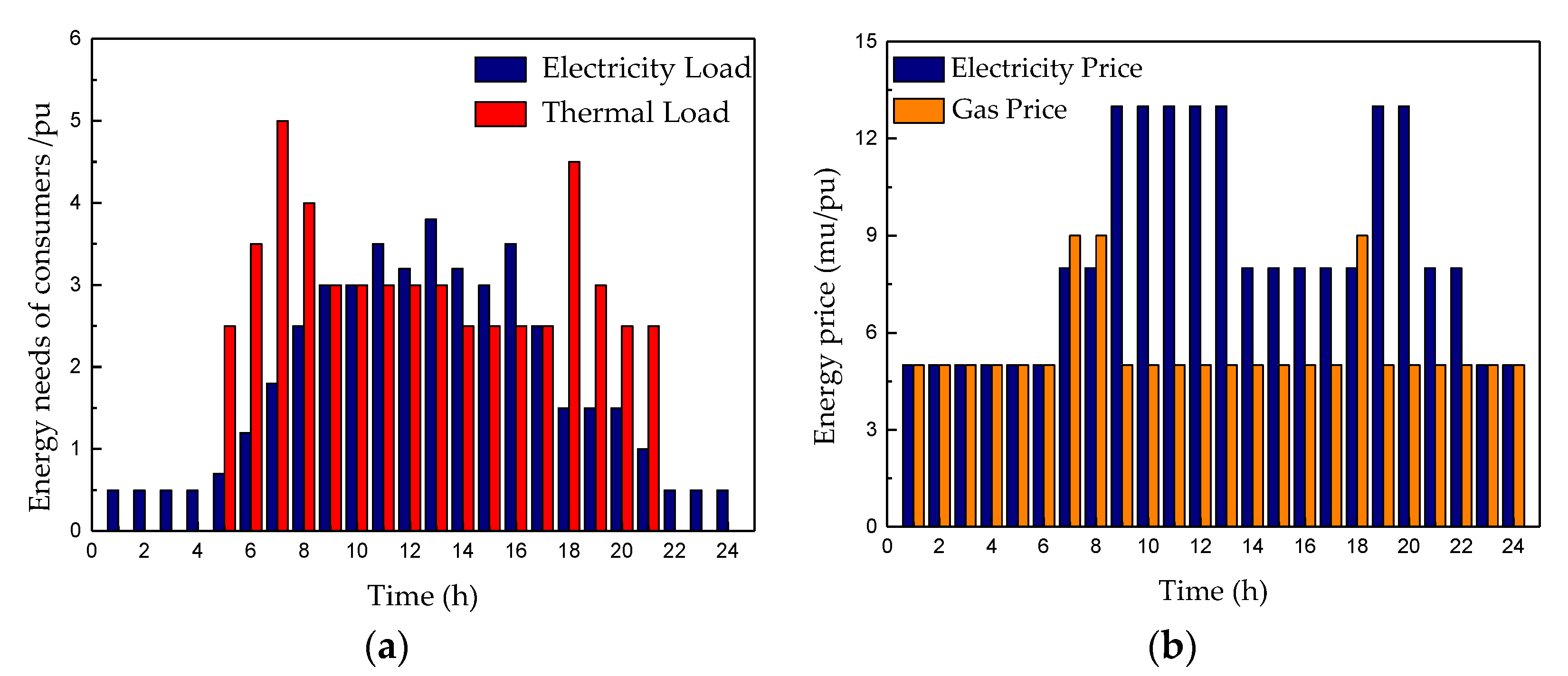
4.1. Parameters for MECS

The parameters of the transformer, MT, gas boiler and heat storage device for the energy facilitator are presented in

Table 2. Parameters for energy facilitator (pu).

Parameters	Value	Parameters	Value	Parameters	Value	Parameters	Value
${\eta }_{\mathrm{ee}}^{\mathrm{T}}$	0.98	$e_h^{-}$	0.9	$P_{\mathrm{gmin}}^{\mathrm{F}}$	0	$\Delta E_{\max ,\mathrm{h}}$	2
${\eta }_{\mathrm{ge}}^{\mathrm{MT}}$	0.35	$P_{\mathrm{emin}}$	0	$P_{\mathrm{gamx}}^{\mathrm{F}}$	5	$E_{\mathrm{loss},\mathrm{h}}$	0.02
${\eta }_{\mathrm{gh}}^{\mathrm{MT}}$	0.45	$P_{\mathrm{emax}}$	10	$E_{\min ,\mathrm{h}}$	0.5	$E_{\mathrm{h}}\left(0\right)$	1
${\eta }_{\mathrm{gh}}^{\mathrm{F}}$	0.9	$P_{\mathrm{gmin}}^{\mathrm{MT}}$	0	$E_{\max ,\mathrm{h}}$	2	-	-
$e_{\mathrm{h}}^{+}$	0.9	$P_{\mathrm{gmax}}^{\mathrm{MT}}$	5	$\Delta E_{\min ,\mathrm{h}}$	−2	-	-

and

Table 3. Parameters for transmission network (pu).

Parameters	Value	Parameters	Value	Parameters	Value	Parameters	Value
$f_{12,\mathrm{e}2}$	0.03	$f_{13,\mathrm{g}3}$	0.02	$F_{\mathrm{g}}^{\min }$	0	$S_{\mathrm{e}2}{}_{\max }$	20
$f_{13,\mathrm{e}2}$	0.06	$f_{42,\mathrm{g}3}$	0.02	$F_{\mathrm{g}}^{\max }$	10	$S_{\mathrm{g}1}{}_{\min }$	0
$f_{42,\mathrm{e}2}$	0.06	$f_{43,\mathrm{g}3}$	0.01	$S_{\mathrm{e}1}{}_{\min }$	0	$S_{\mathrm{g}2}{}_{\min }$	0
$f_{43,\mathrm{e}2}$	0.03	$F_{\mathrm{e}}^{\min }$	0	$S_{\mathrm{e}2}{}_{\min }$	0	$S_{\mathrm{g}1}{}_{\max }$	20
$f_{12,\mathrm{g}3}$	0.01	$F_{\mathrm{e}}^{\max }$	10	$S_{\mathrm{e}1}{}_{\max }$	20	$S_{\mathrm{g}2}{}_{\max }$	20

, the energy loss coefficient of each line and the capacity restrictions of each line and each source are illustrated. Furthermore, the predicted energy needs of the energy consumers are shown in Figure 8a. Four energy consumers in Figure 6 have the same energy needs in this paper. The Time of Use (TOU) pricing for electricity and natural gas are utilized for optimal economic dispatch in Figure 8b. In this paper, the units of cost and energy are monetary unit (mu) and per unit (pu), respectively.

4.2. Results and Discussion

Based on the hierarchical optimal scheduling framework in Figure 5, the dispatch results of the MECS are divided into the results in two parts: the energy hub layer and the transmission network layer. The costs of each energy facilitator and the losses on each transmission network for 24 h are summarized in

Table 4. Energy cost for 24 h (mu).

	Energy Facilitator 1	Energy Facilitator 2	Energy Facilitator 3	Energy Facilitator 4	Electricity Network	Gas Network	Sum
Case 1	707.29	706.28	706.55	706.97	14.97	151.12	2993.18
Case 2	716.25	716.25	716.25	716.25	14.52	155.78	3035.30
Case 3	786.09	786.09	786.09	786.13	57.27	35.84	3237.51
Case 4	794.52	794.52	794.52	794.52	57.27	51.45	3286.80

, which indicates that the total cost of Case 1 is lower than the other cases in this paper. Analysis of the results of the two optimization layers leading to the cost in Table 4 is presented in this section.

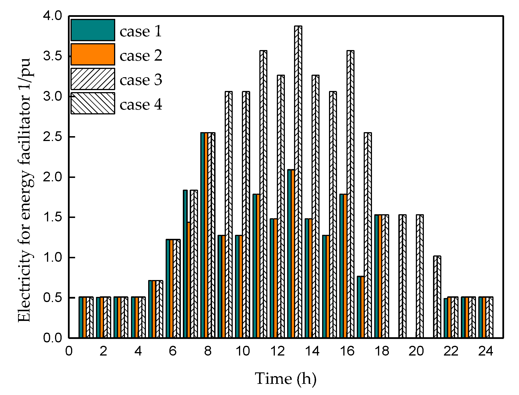
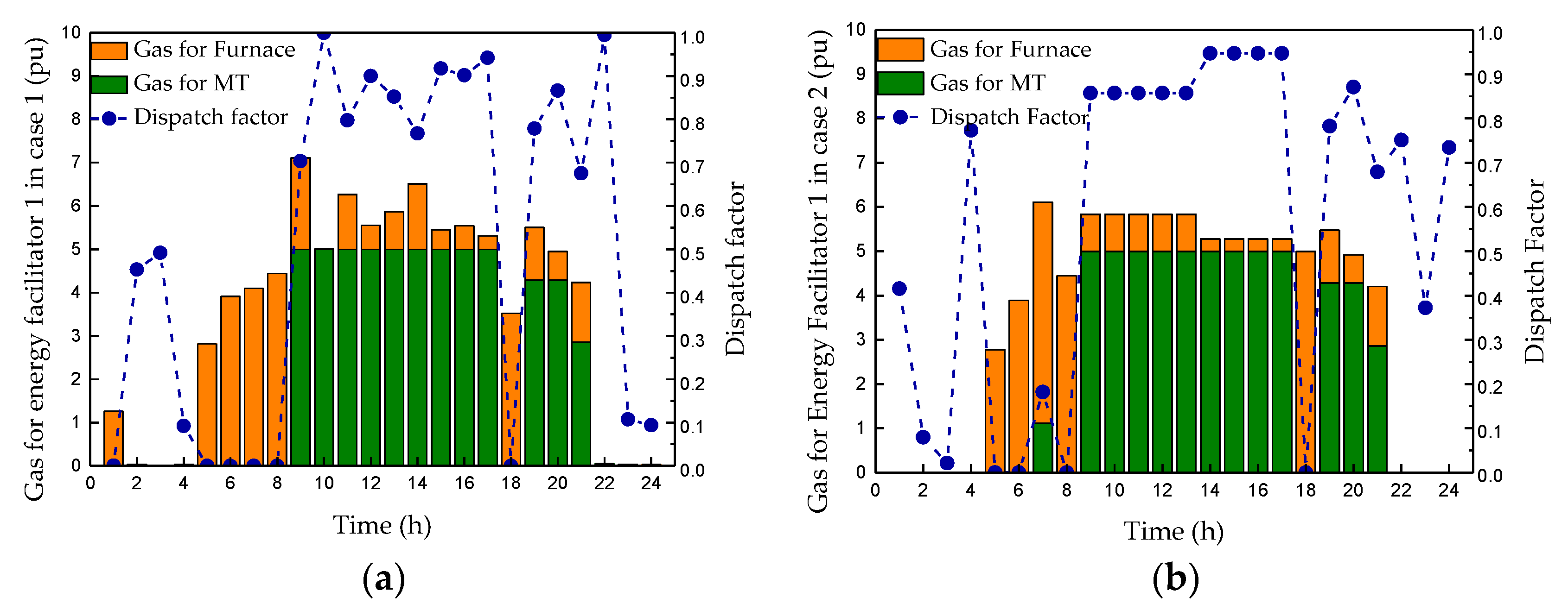
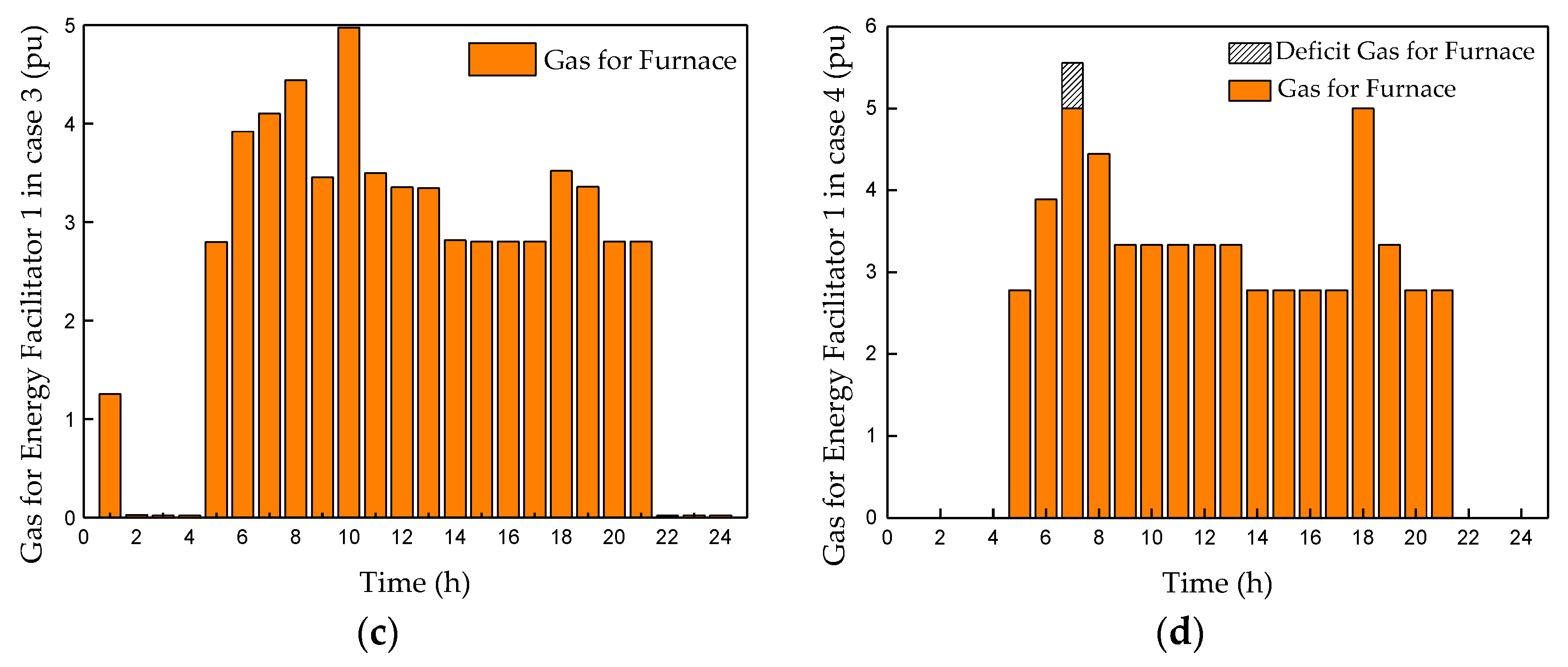
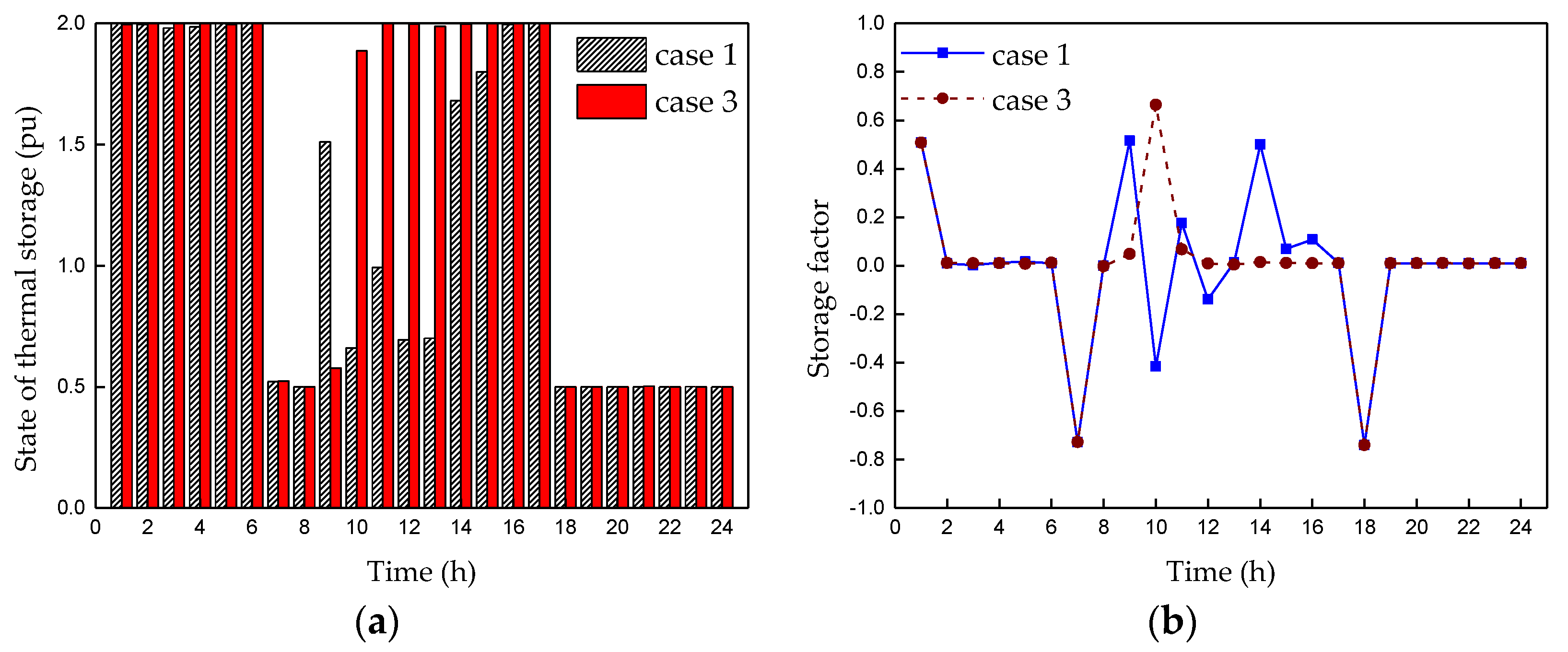
4.2.1. Dispatch Results of the Energy Hub Layer

Since all energy facilitators have the same devices in each case, only the results of Energy Facilitator 1 are introduced and compared in this section. The electricity purchased from the transmission network for each case is shown in Figure 9. In Figure 10, the distribution of natural gas for the MT and the gas boiler, and the dispatch factor are illustrated. For the heat storage devices in Case 1 and Case 3, the operation states and storage factors are described in Figure 11.

During the periods (1:00–4:00, 22:00–24:00) without heat loads, natural gas is not employed for Cases 2 and 4 because the heat storage devices are not integrated into the energy facilitators. On the contrary, for Cases 1 and 3 containing heat storage devices, most of the natural gas is distributed to the gas boiler for heat production and stored due to the low natural gas price, as shown in Figure 10a,c. In addition, the MT does not work, not only in these two periods but also in the period (5:00–6:00), as shown in Figure 10a,b. The main reasons for this are that the electricity price and natural gas price are relatively low, but the efficiencies of the transformer and gas boiler are higher than that of MT. Energy facilitators prefer to choose the transformer and gas boiler to meet the energy needs of the consumers.

During the period (7:00–21:00), the electricity price is higher than the price of natural gas as a whole, as illustrated in Figure 8b. As shown in Figure 9, compared with the Cases 1 and 2, more electricity is purchased from the transmission network in Cases 3 and 4 since MT is not included in producing electricity. However, as described in Figure 10, it is worth mentioning that the natural gas does not flow into the MT at 7:00, 8:00 and 18:00 in Case 1. The major reason for this is that natural gas is more expensive than electricity. To meet the heat needs, energy facilitators prefer to link natural gas to a boiler which has a higher thermal efficiency compared to MT. In addition, the heat storage device would release thermal energy stored when the price of gas was cheap. Moreover, natural gas flows into both the MT and the boiler, to meet the heat load peak at 7:00 in Case 2, even though the gas price is high. The capacity restriction of the gas boiler and the absence of a heat storage device might account for this result; therefore, the energy facilitator should employ the MT to generate heat combined with the gas boiler.

During the period (9:00–12:00), the electricity price is at a peak and the gas price is in a trough. Most of the natural gas would flow into MT to generate electricity for minimizing the cost, as shown in Figure 10a,b. In addition, the heat storage device is employed to balance the heat load, as shown in Figure 11 in Case 1 and Case 3. Also, the consumption of natural gas in Case 2 is less than Case 1 in Figure 10a,b.

The dispatch results of Case 4, as traditional decoupled electricity and heat systems, are described in Figure 9 and Figure 10d. It is worth mentioning that when the heat load is at the highest point, the energy facilitator cannot meet the thermal need of the energy consumer due to the capacity restriction of the gas boiler. However, since either the MT or heat storage device are included in other cases, the heat loads in those cases can be satisfied during the whole dispatch interval.

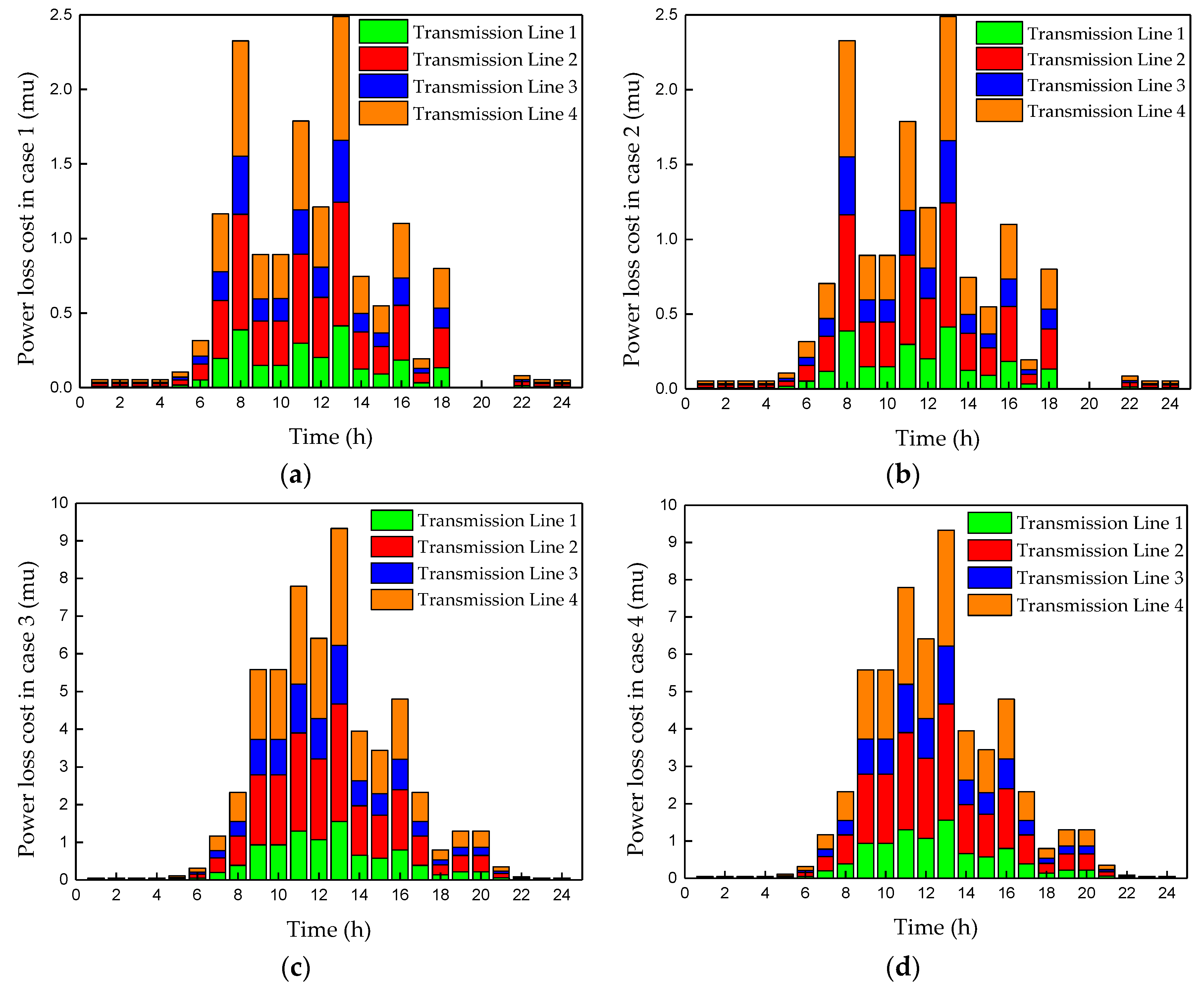
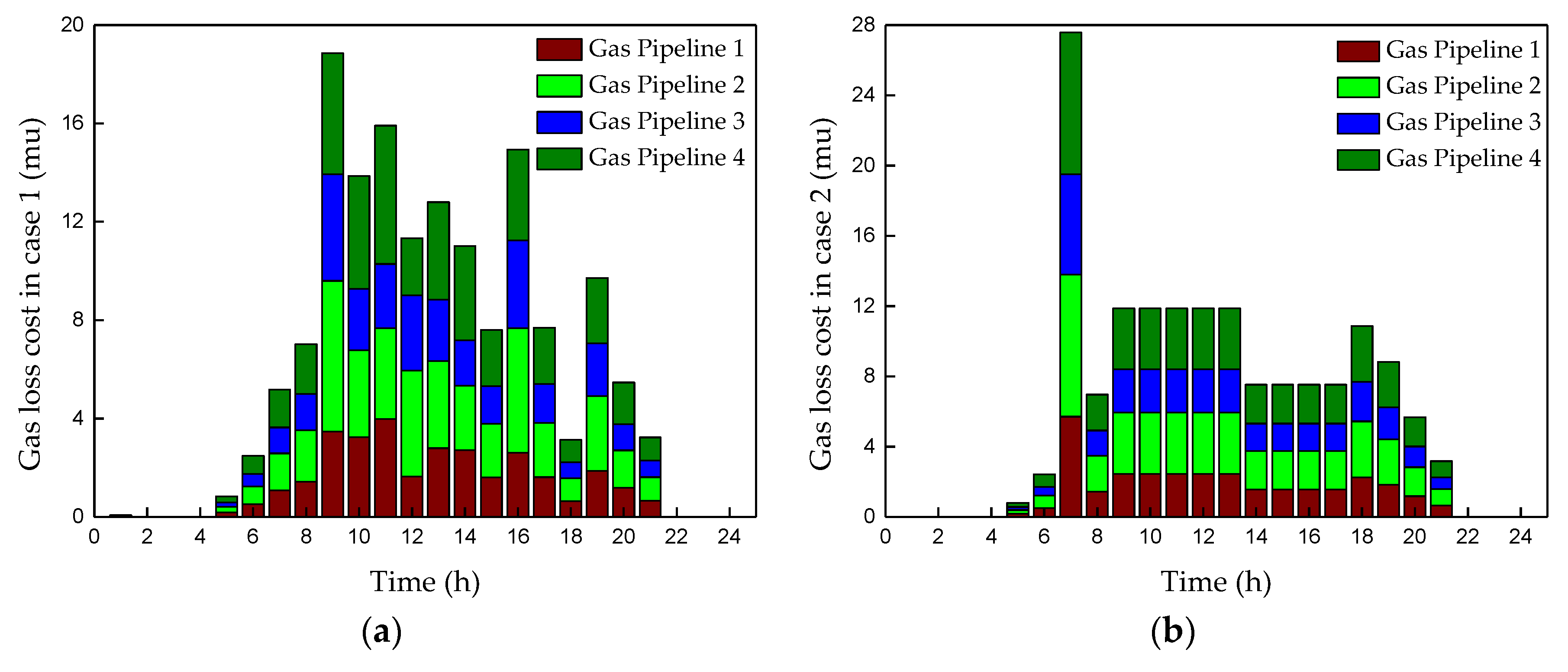
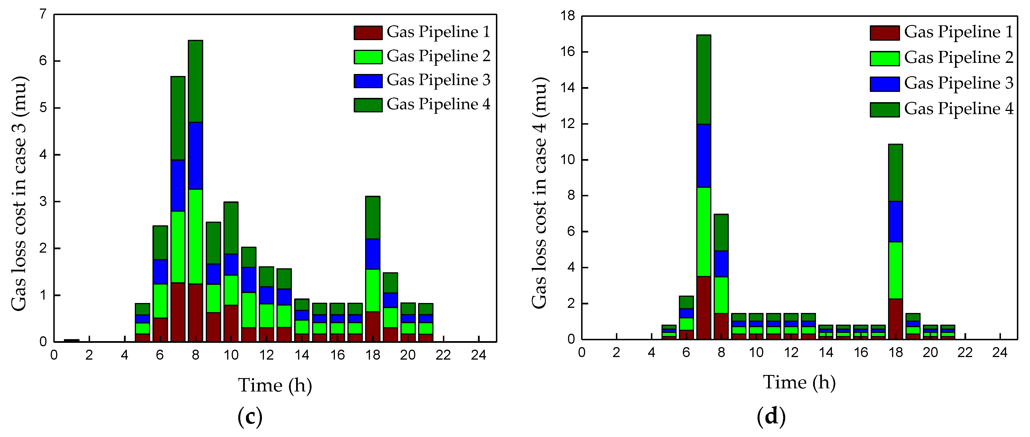
4.2.2. Dispatch Results of the Transmission Network Layer

The costs of power loss in the transmission network in Case 1 and Case 2 are lower than in Case 3 and Case 4 in Table 4, which results from the fact that more electricity is transported at each hour in the latter two cases.

Also, for the consumption of natural gas, Case 1 and Case 2, which are equipped with the MT, demand more gas, as shown in Figure 10, which leads to greater gas loss compared to Case 3 and Case 4.

The electricity purchased from energy providers is similar in Case 1 and Case 2 except at 7:00 (Figure 9). The reason for this result is that the MT is required to coordinate with the gas boiler to meet the peak heat load in Case 2, where there is no heat storage device contained. Therefore, part of the power is generated in the energy facilitator, which means that less electricity comes from the energy provider in Case 2 compared to Case 1, as reflected in the power loss at 7:00 in Figure 12a,b. In Figure 12c,d, it is obvious that the power distribution at each interval and the power loss costs of the transmission network are identical in Case 3 and Case 4 because no other energy carrier is transformed to power energy.

In Case 1, the consumption of natural gas is a little higher than that in Case 2 due to the loss of heat storage device. However, the loss cost of the natural gas network in Case 1 is lower compared to Case 2 in Table 4. The major reason for this result is the regulation of the heat storage device. In Case 1, natural gas could be purchased more and converted to thermal energy by the gas boiler and then stored in the heat storage at a low price. When the natural gas price is high, the storage device could release the thermal energy without gas from the energy provider, resulting in the decrease of gas pipeline loss costs in the transmission network, as described in Figure 13a,b. Therefore, more natural gas is acquired with fewer loss costs due to the high flexibility in Case 1. The loss costs of the natural gas network at each hour are shown in Figure 13c,d, which demonstrate that the heat storage device could reduce the loss costs of the natural gas network. Furthermore, the effect of the heat storage device in decreasing natural gas loss costs is reflected more distinctly in Cases 3 and 4 in Table 4.

5. Conclusions

This paper investigates the modeling, optimal economic operation, and analysis of MECS, which integrates multiple energy carriers. Three interest bodies: the energy provider, energy facilitator, and energy consumer, were investigated by analyzing the structure in MECS. The mathematical model of the energy facilitator was accomplished based on the well-known concept of the energy hub, and the optimal economic operation model of the energy facilitator was carried out. In addition, the optimal economic dispatch model for the multi-carrier transmission network was formulated to minimize the cost of energy providers for each energy carrier.

To acquire the optimal economic operation for both energy facilitator and energy provider, a hierarchical optimal economic operation strategy was formulated to address these two optimization problems. QPSO was employed in the optimal economic scheduling layer for each energy facilitator, and a commercial optimization toolbox was utilized in the optimal economic scheduling layer for energy providers in each energy carrier.

Four cases were designed to verify the effectiveness of the MECS model and the hierarchical optimal economic operation strategy. The acquired results show that compared with the traditional decentralized energy system, MECS could achieve rational distribution and coordination, complement different energy carriers, and decrease the operation cost extensively.

In future work, renewable energy such as wind power and photovoltaic energy will be considered to investigate how intermittency affects the economic behavior of the energy facilitator and energy provider in MECS. Besides, the variable efficiency and dynamic characteristics of equipment will also be investigated.

References

1. Hemmes, K.; Zachariah-Wolf, J.L.; Geidl, M.; Andersson, G. Towards multi-source multi-product energy systems. Int. J. Hydrog. Energy 2007, 32, 1332–1338. [Google Scholar] [CrossRef]
2. Wu, J.; Yan, J.; Jia, H.; Hatziargyriou, N.; Djilali, N.; Sun, H. Integrated energy systems. Appl. Energy 2016, 167, 155–157. [Google Scholar] [CrossRef]
3. Krause, T.; Andersson, G.; Froehlich, K.; Vaccaro, A. Multiple-energy carriers: Modeling of production, delivery, and consumption. Proc. IEEE 2011, 99, 15–27. [Google Scholar] [CrossRef]
4. Mancarella, P. Mes (multi-energy systems): An overview of concepts and evaluation models. Energy 2014, 65, 1–17. [Google Scholar] [CrossRef]
5. Ha, T.T.; Zhang, Y.; Hao, J.; Thang, V.V.; Li, C.; Cai, Z. Energy hub’s structural and operational optimization for minimal energy usage costs in energy systems. Energies 2018, 11, 707. [Google Scholar] [CrossRef]
6. Mohammadi, M.; Noorollahi, Y.; Mohammadi-Ivatloo, B.; Hosseinzadeh, M.; Yousefi, H.; Khorasani, S.T. Optimal management of energy hubs and smart energy hubs—A review. Renew. Sustain. Energy Rev. 2018, 89, 33–50. [Google Scholar] [CrossRef]
7. Geidl, M.; Koeppel, G.; Favre-Perrod, P.; Klockl, B. Energy hubs for the future. IEEE Power Energy Mag. 2007, 5, 24–30. [Google Scholar] [CrossRef]
8. Mohammadi, M.; Noorollahi, Y.; Mohammadi-Ivatloo, B.; Yousefi, H. Energy hub: From a model to a concept—A review. Renew. Sustain. Energy Rev. 2017, 80, 1512–1527. [Google Scholar] [CrossRef]
9. Fabrizio, E.; Corrado, V.; Filippi, M. A model to design and optimize multi-energy systems in buildings at the design concept stage. Renew. Energy 2010, 35, 644–655. [Google Scholar] [CrossRef]
10. Salimi, M.; Ghasemi, H.; Adelpour, M.; Vaez-Zadeh, S. Optimal planning of energy hubs in interconnected energy systems: A case study for natural gas and electricity. IET Gen. Transm. Dis. 2015, 9, 695–707. [Google Scholar] [CrossRef]
11. Zarif, M.; Khaleghi, S.; Javidi, M.H. Assessment of electricity price uncertainty impact on the operation of multi-carrier energy systems. IET Gen. Transm. Dis. 2015, 9, 2586–2592. [Google Scholar] [CrossRef]
12. Rastegar, M.; Fotuhi-Firuzabad, M. Load management in a residential energy hub with renewable distributed energy resources. Energy Build. 2015, 107, 234–242. [Google Scholar] [CrossRef]
13. Paudyal, S.; Cañizares, C.A.; Bhattacharya, K. Optimal operation of industrial energy hubs in smart grids. IEEE Trans. Smart Grid 2015, 6, 684–694. [Google Scholar] [CrossRef]
14. Brahman, F.; Honarmand, M.; Jadid, S. Optimal electrical and thermal energy management of a residential energy hub, integrating demand response and energy storage system. Energy Build. 2015, 90, 65–75. [Google Scholar] [CrossRef]
15. Orehounig, K.; Evins, R.; Dorer, V. Integration of decentralized energy systems in neighbourhoods using the energy hub approach. Appl. Energy 2015, 154, 277–289. [Google Scholar] [CrossRef]
16. Geidl, M.; Andersson, G. A modeling and optimization approach for multiple energy carrier power flow. In Proceedings of the 2005 IEEE Russia Power Tech, St. Petersburg, Russia, 27–30 June 2005; pp. 1–7. [Google Scholar]
17. Bai, L.; Li, F.; Cui, H.; Jiang, T.; Sun, H.; Zhu, J. Interval optimization based operating strategy for gas-electricity integrated energy systems considering demand response and wind uncertainty. Appl. Energy 2016, 167, 270–279. [Google Scholar] [CrossRef] [Green Version]
18. Qiao, Z.; Guo, Q.; Sun, H.; Pan, Z.; Liu, Y.; Xiong, W. An interval gas flow analysis in natural gas and electricity coupled networks considering the uncertainty of wind power. Appl. Energy 2017, 201, 343–353. [Google Scholar] [CrossRef]
19. Zheng, J.H.; Wu, Q.H.; Jing, Z.X. Coordinated scheduling strategy to optimize conflicting benefits for daily operation of integrated electricity and gas networks. Appl. Energy 2017, 192, 370–381. [Google Scholar] [CrossRef]
20. Li, G.; Zhang, R.; Jiang, T.; Chen, H.; Bai, L.; Cui, H.; Li, X. Optimal dispatch strategy for integrated energy systems with cchp and wind power. Appl. Energy 2016, 192, 408–419. [Google Scholar] [CrossRef]
21. Yang, W.; Wen, F.; Wang, K.; Huang, Y.; Salam, M.A. Modeling of a district heating system and optimal heat-power flow. Energies 2018, 11, 929. [Google Scholar] [CrossRef]
22. Liu, X.; Jenkins, N.; Wu, J.; Bagdanavicius, A. Combined analysis of electricity and heat networks. Appl. Energy 2016, 162, 1238–1250. [Google Scholar] [CrossRef]
23. Pazouki, S.; Haghifam, M.R. Optimal planning and scheduling of energy hub in presence of wind, storage and demand response under uncertainty. Int. J. Electr. Power 2016, 80, 219–239. [Google Scholar] [CrossRef]
24. Pazouki, S.; Haghifam, M.R.; Moser, A. Uncertainty modeling in optimal operation of energy hub in presence of wind, storage and demand response. Int. J. Electr. Power 2014, 61, 335–345. [Google Scholar] [CrossRef]
25. Vahid-Pakdel, M.J.; Nojavan, S.; Mohammadi-Ivatloo, B.; Zare, K. Stochastic optimization of energy hub operation with consideration of thermal energy market and demand response. Energy Convers. Manag. 2017, 145, 117–128. [Google Scholar] [CrossRef]
26. Majidi, M.; Nojavan, S.; Zare, K. A cost-emission framework for hub energy system under demand response program. Energy 2017, 134, 157–166. [Google Scholar] [CrossRef]
27. Beigvand, S.D.; Abdi, H.; Scala, M.L.; Yan, J. A general model for energy hub economic dispatch. Appl. Energy 2017, 190, 1090–1111. [Google Scholar] [CrossRef]
28. Shabanpour-Haghighi, A.; Seifi, A.R.; Niknam, T. A modified teaching–learning based optimization for multi-objective optimal power flow problem. Energy Convers. Manag. 2014, 77, 597–607. [Google Scholar] [CrossRef]
29. Shabanpour-Haghighi, A.; Seifi, A.R. Energy flow optimization in multicarrier systems. IEEE Trans. Ind. Inform. 2015, 11, 1067–1077. [Google Scholar] [CrossRef]
30. Shabanpour-Haghighi, A.; Seifi, A.R. Multi-objective operation management of a multi-carrier energy system. Energy 2015, 88, 430–442. [Google Scholar] [CrossRef]
31. Moeini-Aghtaie, M.; Dehghanian, P.; Fotuhi-Firuzabad, M.; Abbaspour, A. Multiagent genetic algorithm: An online probabilistic view on economic dispatch of energy hubs constrained by wind availability. IEEE Trans. Sustain. Energy 2014, 5, 699–708. [Google Scholar] [CrossRef]
32. Moeini-Aghtaie, M.; Abbaspour, A.; Fotuhi-Firuzabad, M.; Hajipour, E. A decomposed solution to multiple-energy carriers optimal power flow. IEEE Trans. Power Systain. 2014, 29, 707–716. [Google Scholar] [CrossRef]
33. Arnold, M.; Negenborn, R.R.; Andersson, G.; Schutter, B.D. Model-based predictive control applied to multi-carrier energy systems. In Proceedings of the IEEE Power & Energy Society General Meeting, Calgary, Canada, 26–30 July 2009; pp. 1–8. [Google Scholar]
34. Chen, Y.; Wang, Y.; Ma, J. Multi-objective optimal energy management for the integrated electrical and natural gas network with combined cooling, heat and power plants. Energies 2018, 11, 734. [Google Scholar] [CrossRef]
35. Geidl, M. Integrated Modeling and Optimization of Multi-Carrier Energy Systems. Ph.D. Thesis, ETH, Zurich, Switzerland, 2007. [Google Scholar]
36. Huang, Y.; Liu, Y.F.; Peng, Z.M.; Ding, Y.J. Research on particle swarm optimization algorithm with characteristic of quantum parallel and its application in parameter estimation for fractional-order chaotic systems. Acta Phys Sin-ch Ed 2015, 64, 030505. [Google Scholar]
37. Sun, J.; Xu, W.; Feng, B. A global search strategy of quantum-behaved particle swarm optimization. In Proceedings of the IEEE Conference on Cybernetics and Intelligent Systems, Singapore, 1–3 December 2004; pp. 111–116. [Google Scholar]
Figure 1. Multi carrier energy system (MECS).
Energies 11 02834 g001
Figure 2. Energy loss model.
Energies 11 02834 g002
Figure 3. Energy storage device.
Energies 11 02834 g003
Figure 4. Energy conversion device.
Energies 11 02834 g004
Figure 5. Hierarchical economic scheduling framework.
Energies 11 02834 g005
Figure 6. A sample case of MECS.
Energies 11 02834 g006
Figure 7. Solution flow chart of MECS.
Energies 11 02834 g007
Figure 8. Energy needs and energy pricing: (a) Electricity loads and thermal loads; (b) time of use (TOU) pricing in MECS.
Energies 11 02834 g008
Figure 9. Electricity supply from electricity network.
Energies 11 02834 g009
Figure 10. Gas supply from the natural gas network: (a) Case 1; (b) Case 2; (c) Case 3; (d) Case 4.
Energies 11 02834 g010aEnergies 11 02834 g010b
Figure 11. Heat storage operation result: (a) State of thermal storage; (b) storage factor.
Energies 11 02834 g011
Figure 12. Power loss cost on the transmission network for different cases: (a) Case 1; (b) Case 2; (c) Case 3; (d) Case 4.
Energies 11 02834 g012
Figure 13. Gas loss cost in the gas network for different cases: (a) Case 1; (b) Case 2; (c) Case 3; (d) Case 4.
Energies 11 02834 g013aEnergies 11 02834 g013b