Distribution Network Congestion Dispatch Considering Time-Spatial Diversion of Electric Vehicles Charging

Abstract

With the popularization of electric vehicles, free charging behaviors of electric vehicle owners can lead to uncertainty about charging in both time and space. A time-spatial dispatching strategy for the distribution network guided by electric vehicle charging fees is proposed in this paper, which aims to solve the network congestion problem caused by the unrestrained and free charging behaviors of large numbers of electric vehicles. In this strategy, congestion severity of different lines is analyzed and the relationship between the congested lines and the charging stations is clarified. A price elastic matrix is introduced to reflect the degree of owners’ response to the charging prices. A pricing scheme for optimal real-time charging fees for multiple charging stations is designed according to the congestion severity of the lines and the charging power of the related charging stations. Charging price at different charging station at different time is different, it can influence the charging behaviors of vehicle owners. The simulation results confirmed that the proposed congestion dispatching strategy considers the earnings of the operators, charging cost to the owners and the satisfaction of the owners. Moreover, the strategy can influence owners to make judicious charging plans that help to solve congestion problems in the network and improve the safety and economy of the power grid.

1. Introduction

Usually, the distribution network is managed by the dispatching agency directly [1]. Towards distribution network’s own structural characteristics [2,3], network capacity is sufficient to meet the power demand of distribution network and congestion does not occur [3]. However, with large-scale distributed energy resources (such as distributed generation, energy storage, active loads and controllable loads, etc.) accessing to the distribution network [4], the composition of the active distribution network has changed greatly. In particular, the rapid development of electric vehicles [5] has a significant impact on the distribution network. Owners can flexibly choose their charging time and charging locations, their unrestrained charging behaviors can increase the difficulty of energy balance control. In view of this, congestion can even occur in active distribution network, and this poses a threat to safe operation of the power grid.

In the case of high penetration of distributed energy resources, managing the congestion in active distribution networks can be divided into direct and indirect methods [6]. Direct methods include network reconfiguration [7], reactive power control [8] and active power control [9]. In network reconfiguration, section switches and contact switches are configured in the distribution network. In reactive power control, reactive power compensation devices are used to solve congestion in distribution networks. In active power control, load demand is reduced to solve congestion in the distribution network. Indirect methods include using the day-ahead congestion price [10,11], day shadow price [12], distribution capacity market [13] and flexible service market [14]. In all four methods, the dispatching agency and electric vehicle owners are the market participants. Because the line transmission capacity is the constraint, the dispatching agency adjusts the charging plan of the owners to solve congestion problem in the distribution network.

With the large-scale introduction of electric vehicles into the network, it has been found that the peak period of free charging loads coincides with the peak period of conventional loads, so the load curve appears “peak to peak” [15], which causes congestion in the distribution network. By adjusting the charging fees [16] or using the optimal power flow method to determine the congestion price [17], operators can adjust and coordinate electric vehicle loads based on charging fees or congestion price. Thus, the load of electric vehicles at congested periods can be transferred to non-congested periods. In this way, congestion problems in the distribution network can be solved and owners’ charging cost can be reduced.

The research outlined above only considered electric vehicles as the dispatching target, and did not fully take the response of the owners to the dispatching strategy into account. As the car owners’ charging behaviors are subject to the owners’ private needs, the traditional dispatching method is no longer applicable to electric vehicles [18]. Adjusting the charging fees can stimulate and encourage owners to change their charging behaviors. The dispatching agency can also make use of the elastic coefficient matrix between the changing rate of charging fees and the changing rate of charging power at each period [19]. Moreover, according to the variation in charging fees at each period, the variation in charging power at each period can be obtained.

In this paper, the real-time charging fees optimization of charging stations in different locations is used to guide the owners’ charging behaviors. The strategy aims to solve the congestion problems in the distribution network caused by electric vehicles. Owners avoid charging in the peak load period because of the high charging price, and choose to charge in the low load period because of the low charging price. Thus, the congestion problem in the distribution network is solved while the benefits to both car owners and operators are also taken into consideration.

2. The Solution Strategy for Congestion in Distribution Networks

2.1. Analysis of the Response of Car owners to Charging Fees.

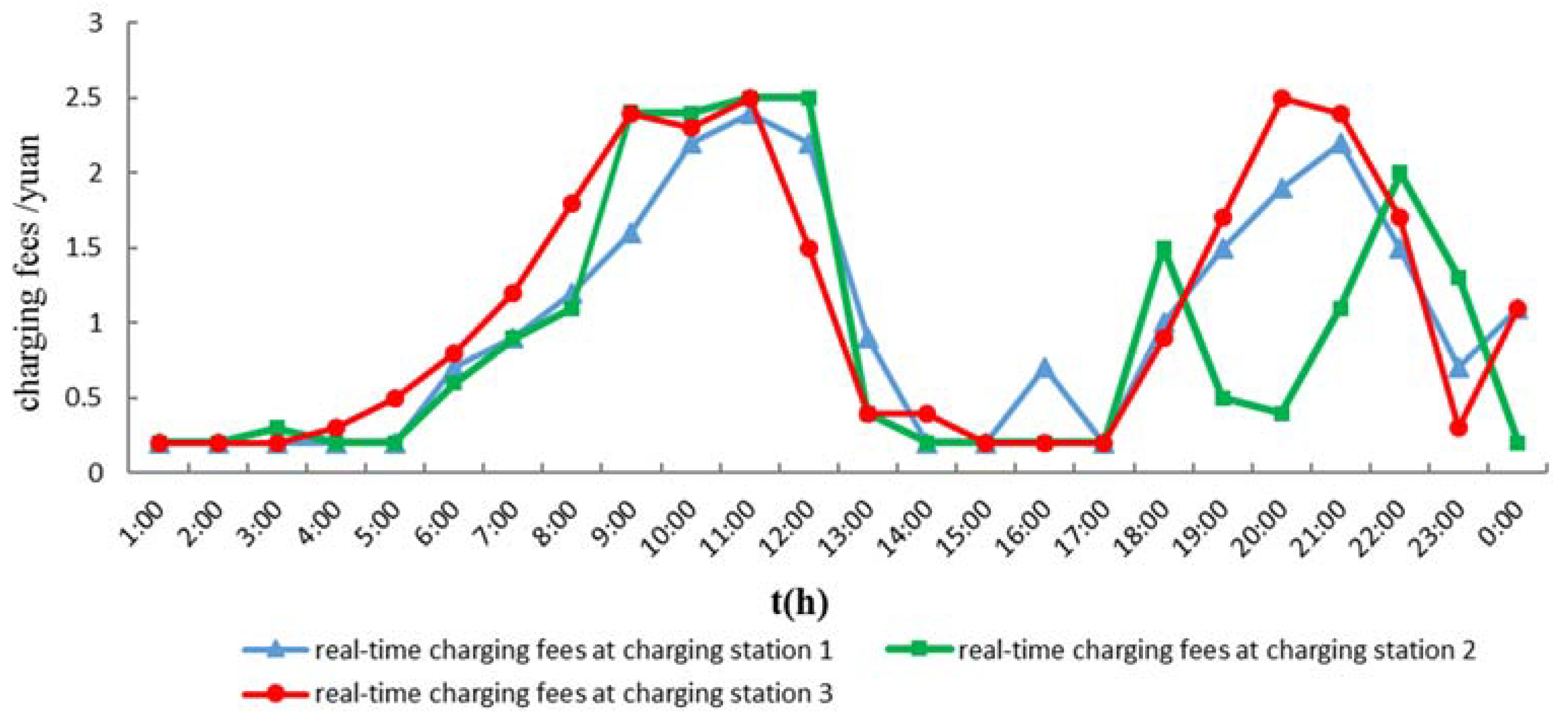
Adjustment of charging fees can influence the charging behaviors of car owners. Thus, the charging power at each period changes. When implementing the policy of real-time charging fees, car owners will respond to the change of charging fees:

$$\mathit{r}=\mathit{E}\cdot \mathit{k},$$

(1)

where $\mathit{r}={\left[r_1{r}_2\cdots r_n\right]}^{\mathrm{T}}$ is the column vector of rate of change of charging power at each period, $r_i=\Delta P_i/P_i(i\in 1,2\dots n)$. $\mathit{k}={\left[k_1{k}_2\cdots k_n\right]}^{\mathrm{T}}$ is the column vector of rate of change of charging fees at each period, $k_i=\Delta p_i/p_i(i\in 1,2\dots n)$. $\mathit{E}=\left[\begin{array}{ccc}{\epsilon }_{11}& \dots & {\epsilon }_{1n}\\ ⋮& \ddots & ⋮\\ {\epsilon }_{n1}& \cdots & {\epsilon }_{nn}\end{array}\right]$ is the elastic coefficient matrix between charging fees and charging power, ${\epsilon }_{ii}=\frac{\partial P_i/P_i}{\partial p_i/p_i}$, ${\epsilon }_{ij}=\frac{\partial P_i/P_i}{\partial p_j/p_j}$, $i,j$ is the different period. $\Delta P_i$ and $\Delta p_i$ are the variation in charging power and the variation in charging fees at $i$ period. $P_i$ is the charging power at $i$ period. $p_i$ and $p_j$ are the charging fees at $i$ and $j$ period.

By setting reasonable real-time charging fees at each time period, according to the known elastic coefficient matrix, the variation in charging power at each period can be obtained. Due to the charging fees, owners will not have their cars charged at the peak load times, thus, the charging load is transferred to other periods to prevent congestion happening in the distribution network.

2.2. Adjustment Strategy for Line Congestion

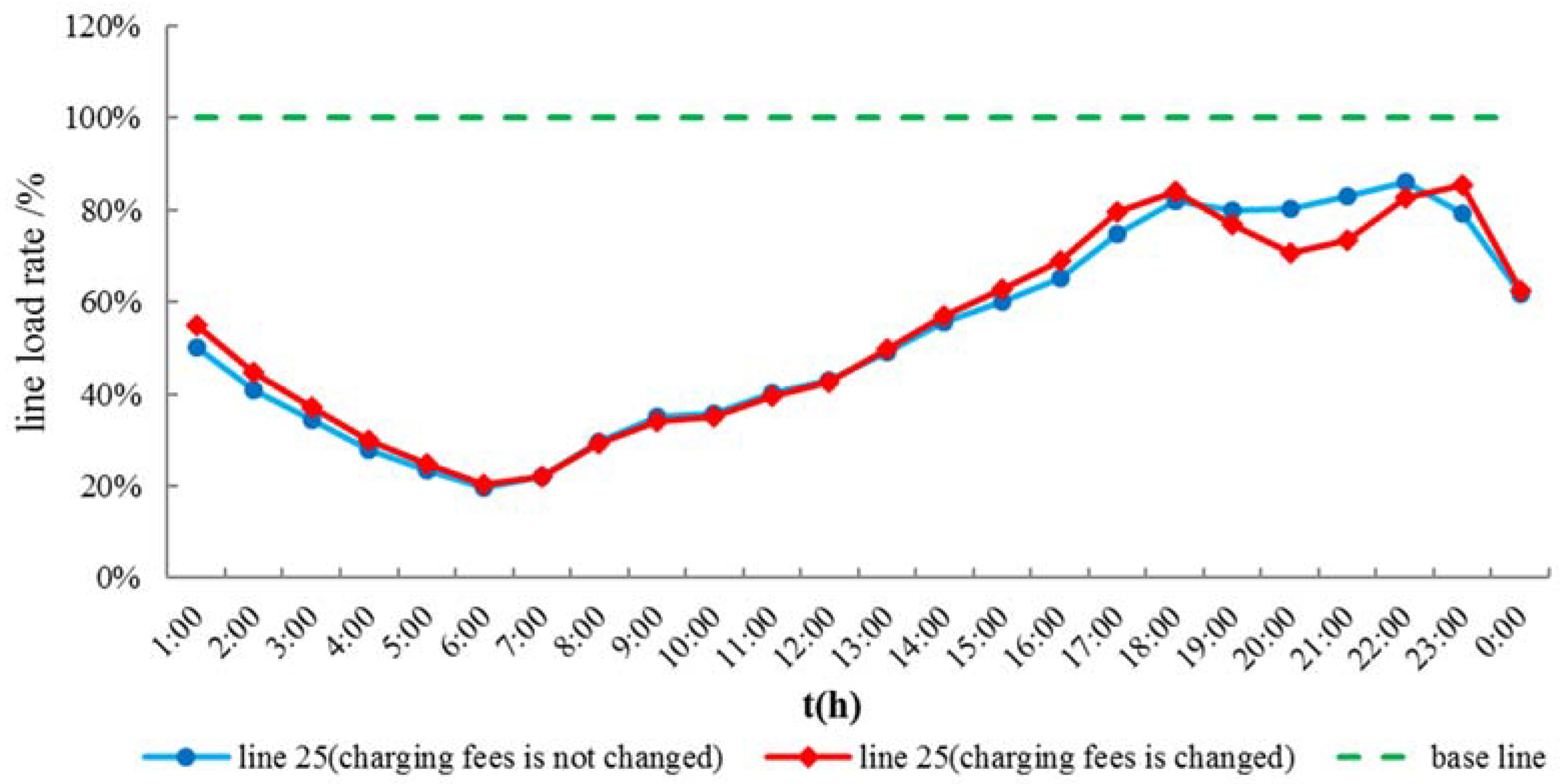
Operators, as market participants, need to check charging plans to avoid congestion in the distribution network. If the charging plans cause congestion in the network, operators will adjust charging fees to guide the charging behaviors of the car owners and solve congestion problem in distribution network.

The “line power needed to be cut” is defined as the basis of judging the degree of line congestion:

$$P_{cut,l,t}=\max \{P_{l,t}-P_{l,\max },0\},$$

(2)

where $P_{cut,l,t}$ is the power needed to be cut of line l at period t, $P_{l,\max }$ is the upper limit of active power of line l, $P_{l,t}$ is the active power of line l at period t, and this can be represented by Equation (3):

$$P_{l,t}=V_{i,t}{V}_{j,t}(G_{ij}\cos {\theta }_{ij,t}+B_{ij}\sin {\theta }_{ij,t})-V_{{}_{i,t}}^2{G}_{ij},$$

(3)

where $V_{i,t}$, $V_{j,t}$ are the voltage amplitude of node $i$ and node $j$ at period t, $G_{ij}$ and $B_{ij}$ are the conductance and susceptance of line $i$ and line $j$. ${\theta }_{ij,t}$ is the difference in voltage phase angle of node $i$ and node $j$ at period t.

In the electric vehicle free charging mode, operators need to verify the charging plans of car owners. Through the power flow calculation, the power flow of each line at each time period can be obtained. Thus, the time period that the congestion occurs and the line number can be obtained.

To reflect the correlation between the charging power of charging stations at different nodes and power lines, the following definitions are given:

Let $M$ be the set of all charging station nodes in the specified area for any subset $M_i\subseteq M$ and its complement is $M_{C,i}$. If there is a power line $l$, its power flow is related to the charging power of the charging station at $\forall m\in M_i$, and is not related to the charging power of the charging station at $\forall m\in M_{C,i}$. In this paper, the line $l$ is the related line of all the charging stations at $M_i$, and all the charging stations at $M_i$ are related to the power line $l$.

A set of lines that meet the above definition is denoted as $l_{M_i}$. If a line in the set is congested at period t, congestion can be solved by reducing the charging power of the charging stations that are related to the line. In order to ensure that all lines in the set are not congested after the adjustment, the reduction of line’s power should be not less than the maximum value of the “line power needed to be cut” in the set, as shown in Equation (4):

$${\displaystyle \sum _{i\in M_i}\left|\Delta P_{cut,i,t}\right|}\ge \underset{l\in l_{M_i}}{\max }(P_{cut,l,t}),$$

(4)

where $\Delta P_{cut,i,t}$ is the reduction of charging power of charging station at node $i$ at period t (in this paper, $\Delta P_{cut,i,t}$ is considered to be negative). The active power loss in the line is ignored in this paper.

The charging power that needs to be cut in the congested period is transferred to other non-congested periods. After the transfer, in order to ensure that new congestion does not occur in the non-congested period, the margin of line power for congestion needs to be considered.

The “margin of line power for congestion” is defined as:

$$P_{margin,l,T}=\max \left\{P_{l,\max }-P_{l,T},0\right\},$$

(5)

where $P_{margin,l,T}$ is the margin of line power for congestion of line l at period $T$, which represents the maximum active power increase that line l can bear without congestion.

In order to ensure all lines which are related to $M_i$ do not have new congestion after adjustment, the transferred charging power should meet the following requirements as shown in Equation (6). The charging power is accepted by each charging station at $M_i$ and in a non-congested period:

$${\displaystyle \sum _{i\in M_i}\Delta P_{margin,i,T}}\le \underset{l\in l_{M_i}}{\min }(P_{margin,l,T}),$$

(6)

where $\Delta P_{margin,i,T}$ is the charging power increase of charging station at node $i$ and non-congested period $T$.

The owners’ response to the adjustment in charging fees is taken into account by the operators. Operators formulate real-time charging fees for each charging station according to the charging power. The charging power needs to be adjusted at each period, as shown in Equation (7).

$$\left[\begin{array}{l}\frac{\Delta P_{i,1}}{P_{i,1}}\\ \frac{\Delta P_{i,2}}{P_{i,2}}\\ ⋮\\ \frac{\Delta P_{i,t}}{P_{i,t}}\end{array}\right]=\mathit{E}\cdot \left[\begin{array}{l}\frac{\Delta p_{i,1}}{p_{i,1}}\\ \frac{\Delta p_{i,2}}{p_{i,2}}\\ ⋮\\ \frac{\Delta p_{i,t}}{p_{i,t}}\end{array}\right],i\in \left(1,2\cdots m\right),$$

(7)

In the equation, there is a total of $m$ charging stations in the area. $P_{i,t}$ is the charging power of the charging station at node $i$ and period t before the implementation of the real-time charging fees policy. $\Delta P_{i,t}$ is the charging power variation of the charging station at node $i$ and period t before and after the implementation of the real-time charging fees policy. Depending on the line congestion state, when the charging station at node $i$ needs to cut the charging power at period t, $\Delta P_{i,t}$ is $\Delta P_{cut,i,t}$. When the charging station at node $i$ needs to accept the transferred charging power at period $T$, $\Delta P_{i,t}$ is $\Delta P_{margin,i,T}$. $p_{i,t}$ is the charging fees of the charging station at node $i$ and period t before the implementation of the real-time charging fees policy. $\Delta p_{i,t}$ is the charging fees variation of charging station at node $i$ and period t before and after the implementation of the real-time charging fees policy. $\mathit{E}$ is the elastic coefficient matrix between charging fees and charging power.

3. Dispatching Model for Active Distribution Network

3.1. Objective Function

When implementing the real-time charging fees policy, operators will pursue the biggest profit while also solving the congestion problem. However, in response to the charging fee adjustment, car owners are likely to be less satisfied compared with the free charging mode. Therefore, car owners hope to maintain high satisfaction while the charging cost is as low as possible.

From the perspective of the operators, the car owners should bear the higher charging cost, while the operators objective is to have the most profit:

$$\max F_1={\displaystyle \sum _{i=1}^m{\displaystyle \sum _{t=1}^n{p^{\prime }}_i(t)}{P^{\prime }}_i(t)},$$

(8)

From the perspective of the owners, their objectives are the minimum charging cost and maximum satisfaction:

$$\min F_2={\displaystyle \sum _{i=1}^m{\displaystyle \sum _{t=1}^n{p^{\prime }}_i(t)}{P^{\prime }}_i(t)},$$

(9)

$$\max F_3=1-\frac{{\displaystyle \sum _{i=1}^m{\displaystyle \sum _{t=1}^n\left|{P^{\prime }}_i\left(t\right)-P_i\left(t\right)\right|}}}{{\displaystyle \sum _{i=1}^m{\displaystyle \sum _{t=1}^n{P}_i\left(t\right)}}},$$

(10)

where ${p^{\prime }}_i(t)$ is the charging fees of the charging station at node $i$ and period t after the implementation of the real-time charging fees policy. ${P^{\prime }}_i(t)$ is the charging power of the charging station at node $i$ and period t after the implementation of the real-time charging fees policy. $P_i(t)$ is the charging power of the charging station at node $i$ and period t before the implementation of the real-time charging fees policy.

In the optimization model, the three objectives of Equations (8)–(10) affect each other. Restrained by system security and power flow balance, when the single objective is optimal, other objectives will be sacrificed as part of the economy. There are often local conflicts between the three objectives [20], which is a typical multi-objective optimization (MOP) problem [21]. The above MOP can be solved by the weighted minimum modulus ideal point method.

$$\min F={\delta }_1\cdot \left|\frac{(-F_1)-(-F_1^{\ast })}{-F_1^{\ast }}\right|+{\delta }_2\cdot \left|\frac{F_2-F_2^{\ast }}{F_2^{\ast }}\right|+{\delta }_3\cdot \left|\frac{(-F_3)-(-F_3^{\ast })}{-F_3^{\ast }}\right|,$$

(11)

$${\delta }_1+{\delta }_2+{\delta }_3=1,$$

(12)

In Equation (12), ${\delta }_1$, ${\delta }_2$, ${\delta }_3$ are the weighted factors of each objective.

In the process of finding the ideal point of the multi-objective function, the objective function $F_1$, $F_2$, $F_3$ are solved to get the optimal solution $F_1^{\ast }$, $F_2^{\ast }$, $F_3^{\ast }$. Then, the objective function $F$ is solved. In the solution process, the objective function has an absolute value term, which is not a smooth differentiable function. It cannot be directly solved by the interior point method. In this paper, the penalty term is smoothed by the aggregate function [22]; then, the optimal solution of $F$ can be obtained.

3.2. The Constraints

1. Multi-time power flow balance constraints:

$$P_{Gi,t}-P_{Di,t}-{P^{\prime }}_{i,t}-V_{i,t}{\displaystyle \sum _{j=1}^N{V}_{j,t}(G_{ij}\cos {\theta }_{ij,t}+B_{ij}\sin {\theta }_{ij,t})=0},$$

(13)

$$Q_{Gi,t}-Q_{Di,t}-V_{i,t}{\displaystyle \sum _{j=1}^N{V}_{j,t}(G_{ij}\sin {\theta }_{ij,t}-B_{ij}\cos {\theta }_{ij,t})}=0,$$

(14)

where $P_{Gi,t}$, $Q_{Gi,t}$, $P_{Di,t}$, $Q_{Di,t}$, ${P^{\prime }}_{i,t}$ is the active power output, reactive power output, active power load, reactive power load, power load of node $i$ at period t, respectively. N is the number of system nodes. $V_{i,t}$, $G_{ij}$, $B_{ij}$, ${\theta }_{ij,t}$ is the voltage amplitude of node $i$ at period t, Conductance and susceptance of line $i,j$ is the difference in voltage phase angle of node $i$ and $j$ at period t.

2. Upper and lower limits of generator power outputs:

$$P_{Gi}^{\min }\le P_{Gi,t}\le P_{Gi}^{\max },$$

(15)

$$Q_{Gi}^{\min }\le Q_{Gi,t}\le Q_{Gi}^{\max },$$

(16)

where $P_{Gi}^{\max }$ and $P_{Gi}^{\min }$ are the upper and lower limits of active power outputs of generator $i$, respectively. $Q_{Gi}^{\max }$ and $Q_{Gi}^{\min }$ are the upper and lower limits of reactive power outputs of generator $i$, respectively.

3. Upper and lower limits of node voltage amplitude:

$$V_i^{\min }\le V_{i,t}\le V_i^{\max },$$

(17)

where $V_i^{\max }$ and $V_i^{\min }$ are the upper and lower voltage amplitude limits of node $i$, respectively.

4. Constraint for overall charging power of all charging stations in the area in one day:

$${\displaystyle \sum _{i=1}^m\Delta P_{i,1}+\Delta P_{i,2}+\cdots +\Delta P_{i,t}}=0,$$

(18)

where $\Delta P_{i,t}$ is the same as in Equation (7). The physical meaning of the Equation (18) is that the sum of the charging power of all charging station in the area in one day is constant before and after the implementation of the real-time charging fees policy.

5. Constraints for charging fees:

$$p^{\min }\le {p^{\prime }}_{i,t}\le p^{\max },$$

(19)

where $p^{\max }$ and $p^{\min }$ are the upper and lower limits of charging fees, respectively. ${p^{\prime }}_{i,t}$ is the charging fees of charging station at node $i$ and period t after the implementation of the real-time charging fees.

6. Constraints for the charging power reduction and increase of each charging station at each period is shown in Section 2.2, Equations (4) and (6).

7. Constraints for the owners’ response to the charging fees adjustment are shown in Section 2.2, Equations (4) and (6).

The process of implementing the real-time charging fees policy is as follows.

Firstly, we can obtain the charging power distribution of the charging station in electric vehicle (EV) free charging mode by a Monte Carlo simulation performed by using the known probability density function of the initial charging time of the electric vehicle and the probability density function of daily mileage.

Secondly, operators will verify the charging plans of owners. After combining the electric vehicle load with the standard load, through the power flow calculation, the power flow of each line at each period can be obtained; thereby, the period and the line number at which the congestion occurs can be obtained.

Then, we can calculate the “line power needed to be cut” of different congested lines at different periods and the “margin of line power for congestion” of different non-congested lines at different periods. So, we can determine the constraints for the reduction of charging power of each charging station at congested period and the constraints for increasing the charging power of each charging station at non-congested period.

Last, taking into account the interests of the owners and operators, the operators optimize the real-time charging fees for each charging station.

To sum up, the congestion dispatching model for active distribution network is shown in Figure 1:

4. Example Verification

4.1. Example System Structure

The modified IEEE-33 system [23] with electric vehicle aggregators and distributed energy resources is shown in Figure 2. The system contains three charging stations, which are located on node 4, node 23 and node 27, respectively. It is assumed that a fixed number of electric vehicles, expressed by the term aggregator, will be charged at each charging station every day in free charging mode. A gas turbine with a capacity of 300 kW is located on node 4, and two wind turbines with installed capacity of 1 MW and 500 kW are located on node 25 and node 28, respectively. A Beta distribution model based on local error [24] is adopted for wind power output. Two photovoltaic power generation units with installed capacity of 500 kW are located on node 15 and node 22. The light intensity meets the Beta distribution [25].

For simplicity, it is assumed that the characteristics and parameters of electric vehicles in different aggregators are the same.

In the example, the weighted factors are taken as ${\delta }_1$ = 0.5, ${\delta }_2$ = 0.3, ${\delta }_3$ = 0.2. The charging fees in free charging mode remains constant at each time period of the day, which is taken as 1 yuan/$\mathrm{kW}\cdot \mathrm{h}$. The elastic coefficient matrix in this paper were obtained from the literature [26]. This needs to be investigated by combining the specific urban economic level, resident income and other factors when it is applied in practice.

4.2. Free Charging Mode for Electric Vehicles

In order to study the impact of large-scale electric vehicles access to the distribution network, the free charging mode is simulated. Monte Carlo simulation is performed by using the known probability density function of the initial charging time of electric vehicles and the probability density function of daily mileage [15]. The distribution results for the charging power of each aggregator is shown in Figure 3.

4.3. Adjustment Mode for Charging Fees

After implementing the real-time charging fees policy, the distribution of charging power of each aggregator is shown in Figure 4. The charging power of each charging station at each period before and after the adjustment for charging fees is shown in

Table A1. Charging power of each charging station at different periods in EV free charging mode.

T	Charging Power of Charging Station 1/kW	Charging Power of Charging Station 2/kW	Charging Power of Charging Station 3/kW	Sum of Charging Power of All Charging Stations
1:00	388.80	291.60	291.60	972.00
2:00	306.18	229.64	229.64	765.45
3:00	230.85	173.14	173.14	577.13
4:00	170.10	127.58	127.58	425.25
5:00	137.70	103.28	103.28	344.25
6:00	101.25	75.94	75.94	253.13
7:00	81.00	60.75	60.75	202.50
8:00	68.85	51.64	51.64	172.13
9:00	56.70	42.53	42.53	141.75
10:00	42.12	31.59	31.59	105.30
11:00	41.31	30.98	30.98	103.28
12:00	55.08	41.31	41.31	137.70
13:00	94.77	71.08	71.08	236.93
14:00	137.70	103.28	103.28	344.25
15:00	202.50	151.88	151.88	506.25
16:00	299.70	224.78	224.78	749.25
17:00	413.10	309.83	309.83	1032.75
18:00	534.60	400.95	400.95	1336.50
19:00	631.80	473.85	473.85	1579.50
20:00	672.30	504.23	504.23	1680.75
21:00	676.35	507.26	507.26	1690.88
22:00	658.53	493.90	493.90	1646.33
23:00	567.00	425.25	425.25	1417.50
00:00	472.23	354.17	354.17	1180.58
sum	7040.52	5280.39	5280.39	17601.30

and

Table A2. Charging power of each charging station at different periods after adjustment for charging fees.

T	Charging Power of Charging Station 1/kW	Charging Power of Charging Station 2/kW	Charging Power of Charging Station 3/kW	Sum of Charging Power of All Charging Stations
1:00	466.89	324.34	362.19	1153.42
2:00	367.66	255.41	285.23	908.30
3:00	277.18	187.77	214.13	679.08
4:00	204.26	141.85	156.94	503.05
5:00	164.81	114.69	121.84	401.35
6:00	108.90	77.66	83.66	270.22
7:00	83.46	57.92	61.98	203.35
8:00	66.58	46.17	44.42	157.16
9:00	49.87	25.90	31.37	107.14
10:00	30.87	19.11	23.91	73.89
11:00	28.26	18.04	21.98	68.27
12:00	41.06	23.89	39.22	104.17
13:00	98.17	76.22	84.26	258.65
14:00	165.12	113.75	124.26	403.13
15:00	243.14	168.88	188.61	600.63
16:00	328.02	250.00	279.08	857.10
17:00	496.07	344.63	384.87	1225.57
18:00	536.73	321.20	430.97	1288.90
19:00	561.74	490.74	426.67	1479.15
20:00	542.61	532.08	361.73	1436.42
21:00	501.19	462.62	366.21	1330.01
22:00	585.44	343.70	442.23	1371.37
23:00	609.13	364.53	519.18	1492.84
00:00	470.51	390.95	366.64	1228.10
sum	7027.65	5152.06	5421.59	17601.30

in Appendix A.

Table 1. Relationship between line number and node number.

Line	Head Node	End Node
1	1	2
2	2	3
3	3	4
4	4	5
5	5	6
22	3	23

shows the relationship between line number and node number,

Table 2. Correlation between line power flow and charging power of the charging station.

Line	Charging Station 1 (Node 4)	Charging Station 2 (Node 23)	Charging Station 3 (Node 27)
1	1	1	1
2	1	1	1
3	1	0	1
4	0	0	1
5	0	0	1
22	0	1	0
25	0	0	1
26	0	0	1

shows the correlation between line power flow and charging power of the charging station. In Table 2, ”1” refers to the power flow of the line that is related to the charging power of charging station, ”0” refers to the power flow of the line that is not related to the charging power of charging station. After superimposing the charging load with the conventional load and the power flow calculation, it can be seen that congestion occurs in line 1, 2, 3, 22, and no congestion occurs in line 4, 5, 25, 26.

Take line 1, which is most likely to congest as an example, as shown in Figure 5.

The congestion problem of the congested lines is solved, and lines 2, 3 and 22 are the same as line 1. It can be seen from line 4 that after the charging load is transferred, the non-congested line still has no congestion, as shown in Figure 6. Lines 5, 25, 26 are the same as line 4. Curves of line load rate for lines 2, 3, 22, 5, 25, 26 before and after adjustment for charging fees are shown in Appendix A, Figure A1, Figure A2, Figure A3, Figure A4, Figure A5 and Figure A6.

The real-time charging fees for three charging stations after optimization is shown in Figure 7. In the case of free charging mode, the charging cost of the owner is 17,601 yuan. After implementing the real-time charging fees policy, the charging cost is 15,433 yuan, and the owners have a high satisfaction rate of 85%. The congestion problem of the distribution network is solved while taking into account the interests of the owners and the operators.

Table 3. Charging power comparison of each charging station before and after the policy.

Sum of Charging Power of Respective Charging Station in a Day	Aggregator 1/kW	Aggregator 2/kW	Aggregator 3/kW	Sum
charging fees is not changed	7040.52	5280.39	5280.39	17601.3
charging fees is changed	7027.65	5152.061	5421.587	17601.3

shows the comparison of the sum of the charging power of the respective charging station for a day before and after the implementation of the real-time charging fees policy.

After the implementation of the real-time charging fees policy, the security and stability of the system operation are improved. This can be seen from

Table 4. Maximum line load rate of a congested line in a day before and after adjustment for charging fees.

Line	Charging Fees Is Not Changed	Charging Fees Is Changed
1	106.10%	98.66%
2	108.31%	99.52%
3	109.98%	99.53%
22	114.06%	99.96%

,

Table 5. Standard deviation of active power of a line before and after adjustment for charging fees.

Line	Charging Fees Is Not Changed	Charging Fees Is Changed
1	1397.51	1348.92
2	1220.94	1170.20
3	795.07	755.02
4	597.03	582.18
5	597.37	586.93
22	401.90	389.50
25	324.74	314.80
26	317.88	308.23

and

Table 6. Peak valley difference of active power of a line before and after adjustment for charging fees.

Line	Charging Fees Is Not Changed	Charging Fees Is Changed
1	4105.38	3745.68
2	3606.44	3228.44
3	2390.13	2071.42
4	1781.16	1614.03
5	1772.11	1768.79
22	1196.42	1045.60
25	995.96	977.49
26	972.12	957.07

.

5. Discussion

As can be seen in Figure 3, the peak of the charging load and the peak of conventional load coincide, resulting in an increase in the peak-to-valley difference in the load curve and a decrease in the utilization efficiency of the power resources.

Figure 5 shows that before the implementation of the real-time charging fees policy, from 19:00 to 22:00, line 1 is in a congested state, and a large amount of power needs to be transmitted from the main network to meet the electricity demand of charging load and conventional load. From 4:00 to 8:00, the lower line load rate is because the electric vehicle load and the conventional load in the network are less. The wind power, photovoltaic power generation units and gas turbine contained in the system can supply part of the power demand, thus the power purchase from the main network and the consumption of fossil fuel can be reduced. It can be seen from line 1 that after the implementation of the real-time charging fees policy, the charging load in the congested period is transferred to the non-congested period.

In Figure 7, it can be seen that the charging station will set low charging fees in the period of low load, and set high charging fees in the period of peak load, so as to persuade car owners to transfer their charging time.

Table 3 shows that the sum of the charging power of respective charging station has changed in the day before and after the adjustment. This indicates that the real-time charging fees of respective charging station at different locations in the area has different degrees of attraction to vehicle owners. Some car owners have changed their charging habits and moved between charging stations, which means the space factors are considered.

In Table 4, it can be seen that after implementing the real-time charging fees policy, the maximum line load rate of congested lines in a day is smaller (under 100%). This means that the security of the system operation is improved.

In Table 5 and Table 6, it can be seen that after implementing the real-time charging fees policy, the standard deviation and peak valley difference for the active power of all lines are smaller, so the fluctuation of the load curve is smaller and the stability of the system operation is improved.

6. Conclusions

A time-spatial dispatching model for the distribution network guided by charging fees for electric vehicles is proposed in this paper to solve congestion problems in the distribution network. This model focuses on the establishment of real-time charging fees at different charging stations so that the charging fees and the owners’ response to these fees lead to owners transferring the charging load from peak load to low load periods. Thus, the congestion problem is solved and potential congestion can be avoided. From the simulation results on the improved IEEE-33 system, the following conclusions are drawn.

The introduction of high-penetration electric vehicles has brought great challenges for the safe and stable operation of active distribution networks and sometimes, even congestion problems happen. The elastic coefficient matrix between the charging fees changing rate and charging power changing rate can fully account for the response of car owners to the dispatching strategy. The congestion dispatching strategy established in this paper can effectively solve congestion problems. The model takes into account the benefits for both car owners and operators, but the response of car owners to the dispatching strategy as well. After implementing the real-time charging fees policy, the maximum line load rate of congested lines in a day is smaller (under 100%), so the congestion problem is solved. Moreover, standard deviation and the peak valley difference of the active power of all lines are smaller and the system is more stable. Thus, the security and stability of the system operation are improved.

The model proposed in this paper is aimed at congestion problems caused by large-scale electric vehicles accessing the distribution network. The congestion caused by other kinds of loads, the transfer of electric vehicles between charging stations considering specific spatial factors such as charging equipotential time and distance will be the subject of further research.

References

1. Hu, S.B.; Sun, H.; Peng, F.X.; Zhou, W.; Cao, W.P.; Su, A.L.; Chen, X.D.; Sun, M.Z. Optimization Strategy for Economic Power Dispatch Utilizing Retired EV Batteries as Flexible Loads. Energies 2018, 11, 1657. [Google Scholar] [CrossRef]
2. Ye, R.; Huang, X.L.; Zhang, Z.Q.; Chen, Z.; Duan, R. A High-Efficiency Charging Service System for Plug-in Electric Vehicles Considering the Capacity Constraint of the Distribution Network. Energies 2018, 11, 911. [Google Scholar] [CrossRef]
3. You, Y.; Liu, D.; Yu, W.P. Technology and Its Trends of Active Distribution Network. Autom. Elect. Power Syst. 2012, 36, 10–16. [Google Scholar] [CrossRef]
4. Fan, M.T.; Zhang, Z.P.; Su, A.X. Enabling Technologies for Active Distribution Systems. Proc. CSEE 2013, 34, 12–18. [Google Scholar] [CrossRef]
5. Hu, Z.C.; Song, Y.H.; Xu, Z.W. Impacts and Utilization of Electric Vehicles Integration into Power Systems. Proc. CSEE 2012, 32, 1–10. [Google Scholar] [CrossRef]
6. Huang, S.; Wu, Q.; Liu, Z. Review of congestion management methods for distribution networks with high penetration of distributed energy resources. In Proceedings of the IEEE PES Innovative Smart Grid Technologies Europe, Istanbul, Turkey, 12–15 October 2014. [Google Scholar]
7. Bouhouras, A.S.; Christoforidis, G.C.; Parisses, C. Reducing Network Congestion in Distribution Networks with High DG Penetration via Network Reconfiguration. In Proceedings of the 11th European Energy Market (EEM14), Krakow, Poland, 28–30 May 2014. [Google Scholar]
8. Daroj, K.; Limpananwadi, W. Reactive Power Dispatch scheme evaluation for synchronous based distributed generators to reduce real power loss in distribution systems. In Proceedings of the 2008 IEEE International Conference on Sustainable Energy Technologies, Singapore, 24–27 November 2008. [Google Scholar]
9. Balaraman, S.; Kamaraj, N. Application of Differential Evolution for Congestion Management in Power System. Modern Appl. Sci. 2010, 4, 33–42. [Google Scholar] [CrossRef]
10. O’Connell, N.; Wu, Q.; Østergaard, J. Day-ahead tariffs for the alleviation of distribution grid congestion from electric vehicles. Electr. Power Syst. Res. 2012, 92, 106–114. [Google Scholar] [CrossRef] [Green Version]
11. Verzijlbergh, R.A.; De, V.L.; Lukszo, Z. Renewable Energy Sources and Responsive Demand. Do We Need Congestion Management in the Distribution Grid? IEEE Trans. Power Syst. 2014, 29, 2119–2128. [Google Scholar] [CrossRef]
12. Biegel, B.; Andersen, P.; Stoustrup, J.; Bendtsen, J. Congestion management in a smart grid via shadow prices. IFAC Proc. Vol. 2012, 45, 518–523. [Google Scholar] [CrossRef]
13. Hu, J.; You, S.; Lin, M. Coordinated Charging of Electric Vehicles for Congestion Prevention in the Distribution Grid. IEEE Trans. Smart Grid 2014, 5, 703–711. [Google Scholar] [CrossRef] [Green Version]
14. Zhang, C.; Ding, Y.; Nordentoft, N. A Danish market solution for DSO congestion management through DER flexibility services. J. Modern Power Syst. Clean Energy 2014, 2, 126–133. [Google Scholar] [CrossRef] [Green Version]
15. Tian, L.T.; Shi, S.L.; Jia, Z. A Statistical Model for Charging Power Demand of Electric Vehicles. Power Syst. Technol. 2010, 34, 126–130. [Google Scholar] [CrossRef]
16. Sun, H.; Shen, Z.H.; Zhou, W. Multi-objective Congestion Dispatch of Active Distribution Network Based on Source-load Coordination. Autom. Electr. Power Syst. 2017, 41, 88–95. [Google Scholar] [CrossRef]
17. Liu, W.J.; Wu, Q.W.; Wen, F.S. A Market for Participation of Electric Vehicles and Dispatchable Loads in Distribution System Congestion Management. Autom. Electr. Power Syst. 2014, 38, 26–33. [Google Scholar] [CrossRef]
18. Gao, Y.J.; Wang, C.; Lv, M.K. Optimal time-of-use price model considering satisfaction degree of electric vehicle owners. Electr. Power Autom. Equip. 2014, 34, 8–13. [Google Scholar] [CrossRef]
19. Tong, X.; Guo, C.L.; Zhang, M.Z. Price Guide of Electric Vehicles Charging Based on Cost Function. Electr. Power Constr. 2016, 37, 30–35. [Google Scholar]
20. Hong, B.W.; Guo, L.; Wang, C.S. Model and method of dynamic multi-objective optimal dispatch for microgrid. Electr. Power Autom. Equip. 2013, 33, 100–107. [Google Scholar] [CrossRef]
21. Tan, X.G.; Wang, H.; Zhang, L. Multi-objective Optimization of Hybrid Energy Storage and Assessment Indices in Microgrid. Autom. Electr. Power Syst. 2014, 38, 7–14. [Google Scholar] [CrossRef]
22. Li, X.S. An efficient approach to a class of non-smooth optimization problems. Sci. China 1994, 37, 323–330. [Google Scholar]
23. Sun, H.; Shen, Z.H.; Zhou, W. Congestion dispatch research of active distribution network with electric vehicle group response. Proc. CSEE 2017, 37, 5549–5559. [Google Scholar]
24. Liu, X. Impact of beta-distributed wind power on economic load dispatch. Electr. Power Compon. Syst. 2011, 39, 768–779. [Google Scholar] [CrossRef]
25. Kaplani, E.; Kaplanis, S. A stochastic simulation model for reliable PV system sizing providing for solar radiation fluctuations. Appl. Energy 2011, 97, 970–981. [Google Scholar] [CrossRef]
26. Kirschen, D.S.; Strbac, G.; Cumperayotc, P. Factoring the elasticity of demand in electricity prices. IEEE Trans. Power Syst. 2000, 15, 612–617. [Google Scholar] [CrossRef]
Figure 1. Congestion dispatching model for active distribution network.
Energies 11 02820 g001
Figure 2. IEEE33 node in the modify test system.
Energies 11 02820 g002
Figure 3. Charging power distribution of each aggregator in EV free charging mode.
Energies 11 02820 g003
Figure 4. Charging power distribution of each aggregator after adjustment for charging fees.
Energies 11 02820 g004
Figure 5. Line load rate of line 1 before and after adjustment for charging fees.
Energies 11 02820 g005
Figure 6. Line load rate of line 4 before and after adjustment for charging fees.
Energies 11 02820 g006
Figure 7. Real-time charging fees of each charging station.
Energies 11 02820 g007