Article

Power and Fuel Economy of a Radial Automotive Thermoelectric Generator: Experimental and Numerical Studies

Department of Mechanical Engineering and Industrial Construction, University of Girona, c/Universitat de Girona 4, 17003 Girona, Spain
*
Author to whom correspondence should be addressed.
Current address: Nabla Thermoelectrics, c/Llibertat 71, 17820 Banyoles, Spain.
Energies 2018, 11(10), 2720; https://doi.org/10.3390/en11102720
Submission received: 30 September 2018 / Revised: 8 October 2018 / Accepted: 10 October 2018 / Published: 11 October 2018

Abstract

:
Recent developments of high performance thermoelectric (TE) materials have increased the interest of using this technology to directly convert waste heat into electricity. In the automotive sector, many automotive thermoelectric generators (ATEGs) designs use TE modules (TEMs) with high hot side temperatures to cope with high engine load regimes. Here, we develop a new concept of a radial ATEG that is specifically designed to work with low temperature TEMs, which enables the use of Pb-free modules and reduces the thermal stress of the device. A prototype is built and tested at different regimes in an engine test bench. A numerical model of the ATEG is developed and validated. The consequences of modifying (1) the exchange area between the heat absorber and the exhaust gases and (2) the effective figure of merit of TEMs on the electrical output power and fuel economy are investigated by means of simulations. Results indicate that the maximum fuel economy (1.3%) is not attained at the point of maximum output power (228 W). In terms of fuel economy, the back pressure at the exhaust penalizes high mass flow regimes. We use a dimensionless parameter to analyze the potential of the ATEG for reducing fuel consumption.

1. Introduction

Transport contributes to more than 20% of carbon dioxide (CO2) emissions worldwide [1]. In Europe, this contribution rises up to 27%, becoming the biggest source of carbon emissions and the main cause of air pollution in cities [2]. Since road transport accounts for more than 70% of all transport emissions, the European Union (EU) has defined green (i.e., low-emission) mobility as one of the main challenges of our society [3]. The transition to a low-carbon mobility involves a strategy with several priority actions. One of them is the development of more efficient vehicles that use internal combustion engines (ICEs), since this technology is not expected to decline at mid-term in long-distance transport with heavy-duty vehicles [4].
In ICEs, approximately 1/3 of the consumed primary energy is lost through the exhaust gases [5]. Several technologies aim to recover part of this waste heat to reduce fuel consumption. The most promising ones are organic Rankine cycles (ORCs) and automotive thermoelectric generators (ATEGs) [6].
ATEGs are devices located at the exhaust pipe, and they consist of commercial thermoelectric modules (TEMs) sandwiched between heat absorbers (in contact with exhaust gases) and heat sinks (in contact either with air or with liquid coolant) with the purpose of maintaining a given temperature difference or, equivalently, a heat flux, across them. TEMs directly convert this heat into electricity. The electrical energy generated is stored in batteries and shortens the time of alternator demand. As a consequence, the engine torque that is intended to drive the alternator reduces, and therefore, fuel consumption diminishes.
On the other hand, the heat absorbers of the ATEG may be circular tubes [7], straight fins [8,9,10,11], dimples [12], phase-change pipes [13], etc., and, to some extent, all of them increase the pressure upstream of the exhaust pipe. This back pressure alters the regular functioning of the engine and increases the fuel consumption. This effect may eventually counterbalance the energy savings produced by electrical generation. However, many previous studies on ATEGs have focused only on maximizing ATEG electrical output power, ignoring the effect of the back pressure, and consequently, overestimating its performance.
Table 1 lists very recent experimental studies of ATEGs. The most common design employed in ATEGs distributes commercial TEMs in a way where their hot side surfaces are in contact with longitudinal (with respect to the flow direction) plates that contour the perimeter of the device cross-section (rectangular [7,8,10,12,13,14], square [11] or hexagonal [9]). The main problem of this layout is the high temperature that is achieved during a driving cycle, since hot gases at full load regimes may exceed 500 °C. Since the maximum allowable hot side temperature in bismute telluride TEMs is on the order of 250 °C, several authors have devised mechanisms to avoid damaging TEMs, which are mainly focused on bypassing the ATEG [8,10]. Alternative designs may involve heat pipes [13], so TEMs can be easily assembled without interfering with the exhaust manifold, or cylindrical non-commercial TEMs mounted in a transversal plane inside the exhaust system [15].
Maximum values of fuel economy due to ATEGs are commonly not reported (see Table 1), although values on the order of 1% have been estimated [10]. These are slightly lower values than those claimed by using ORCs (up to 7% [16]), although back pressure and weight effects in real on-vehicle tests may substantially reduce this figure, even leading to increments in fuel consumption [17]. In comparison with ORCs, ATEGs possess the advantages of being simpler, lighter, and more silent, compact, and reliable [6].
Thus, the research in ATEGs is in constant development. Especially in recent years, when ongoing research on new bulk thermoelectric materials has led to a continuous increase of the values of the figure of merit (ZT) that determines the potential to convert heat into electricity. However, there still exists a gap between the efficiency of these bulk materials and commercial TEMs, which are formed by hundreds of p-type and n-type thermoelectric legs, electrically conductive junctions, and electrically isolating plates [18]. TEMs also suffer from thermal stress due to the continuous exposure to low and high temperature cycles [18]. This applies not only to each individual component of the TEM, but also to the overall module because of the mismatch in the thermal expansion coefficient of the materials used. Thus, in order to avoid TEM failure and to assure long-term mechanical stability, the temperature variations applied to the TEM should be minimized [19]. However, and in order (1) to extract the maximum available heat of exhaust gases, and (2) to avoid not being overheated, some previous ATEG designs use high temperature TEMs (nominal hot side temperature on the order of 500 °C) [7]. These high temperature TEMs often use Pb in the semiconductors, unable to be present in commercial devices due to environmental reasons.
Thus, the purpose of the present paper aims to address the two issues regarding ATEGs that have been stated above: (1) to develop a novel ATEG design able to work with low temperature Pb-free commercial TEMs, and (2) to analyze the ATEG performance in terms of fuel consumption rather than on electrical output power.
The design consists of a radial ATEG whose main novelty is that the TEMs are not faced towards the exhaust pipe, but they are distributed in a transversal plane to the flow. This layout avoids the overheating of TEMs in high engine load regimes without adding any mechanical part, and allows us to use low-temperature TEMs. This radial ATEG is explained in detail in Section 2, where we also carry out an experimental study in an engine test bench. Section 3 describes and validates the numerical model that is used to simulate the ATEG. Numerical simulations under different scenarios (changes in TEMs performance and in fin dimensions of the heat absorbers) are analyzed in Section 4, which also includes a discussion focused on the fuel economy. Finally, the main conclusions are found in Section 5.

2. Experimental Analysis
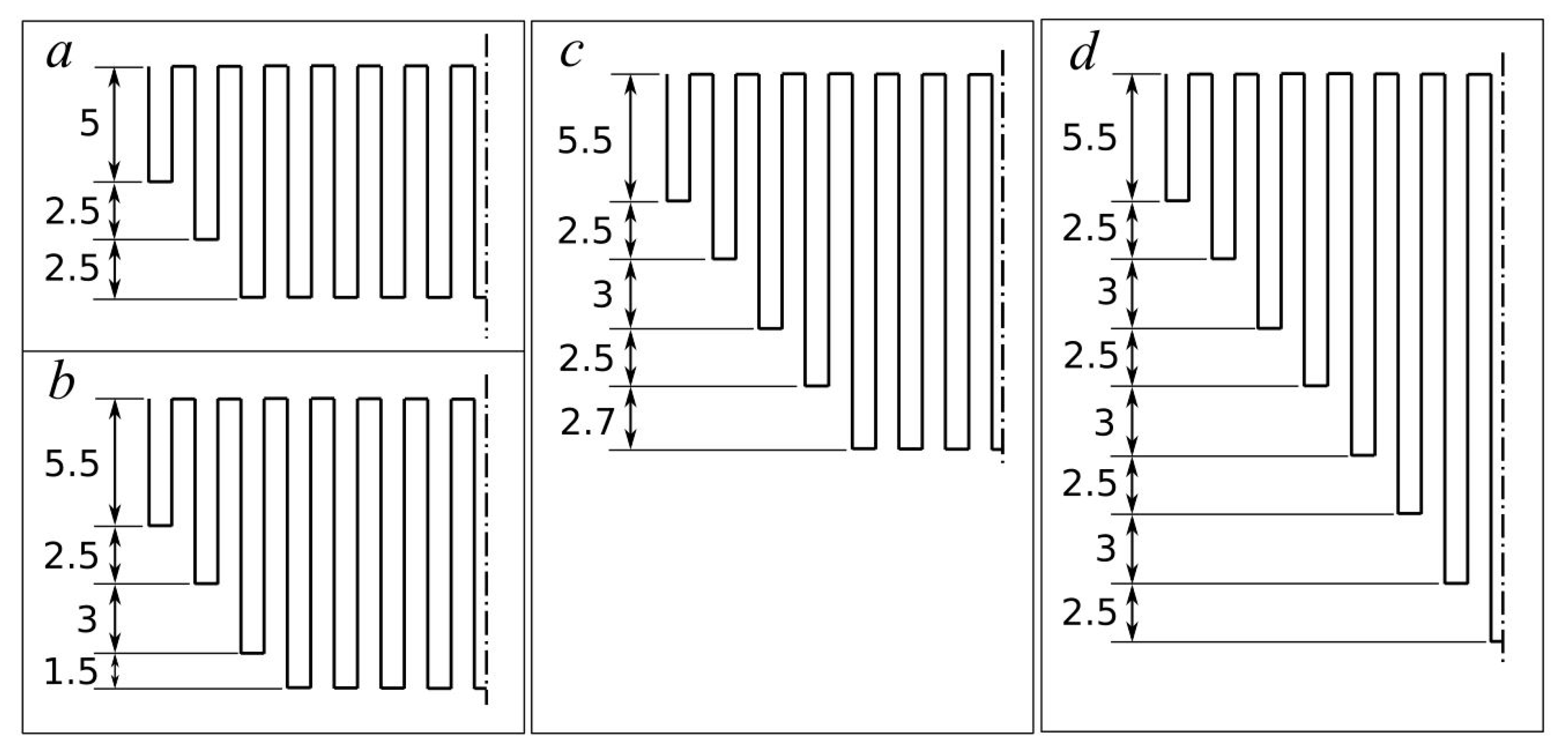
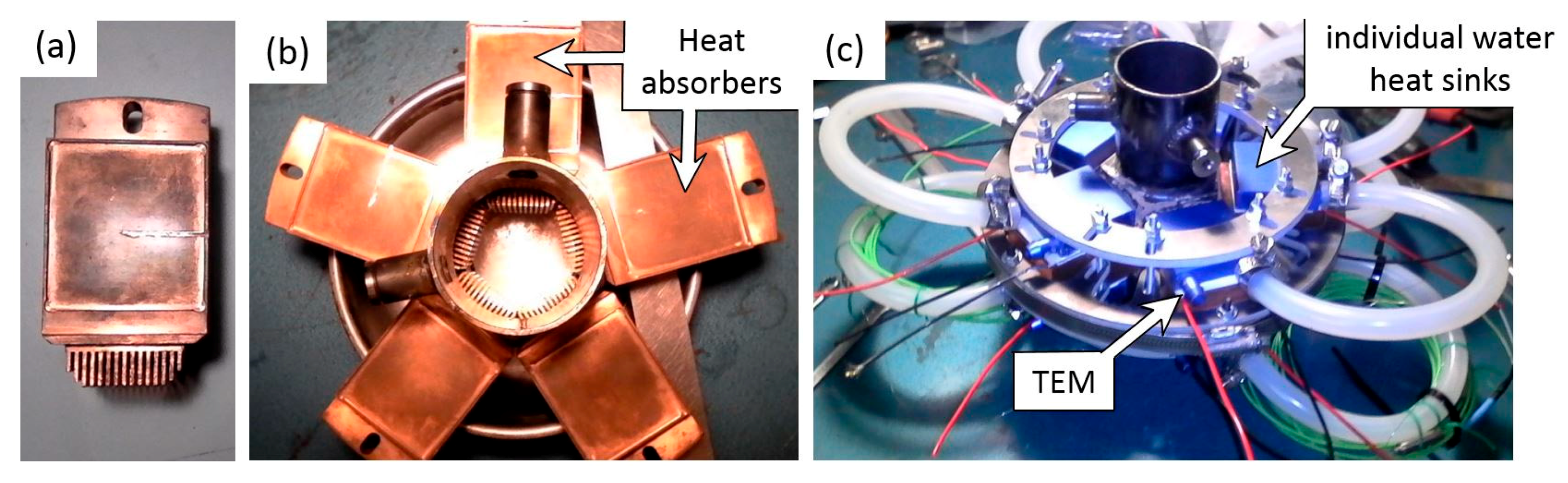
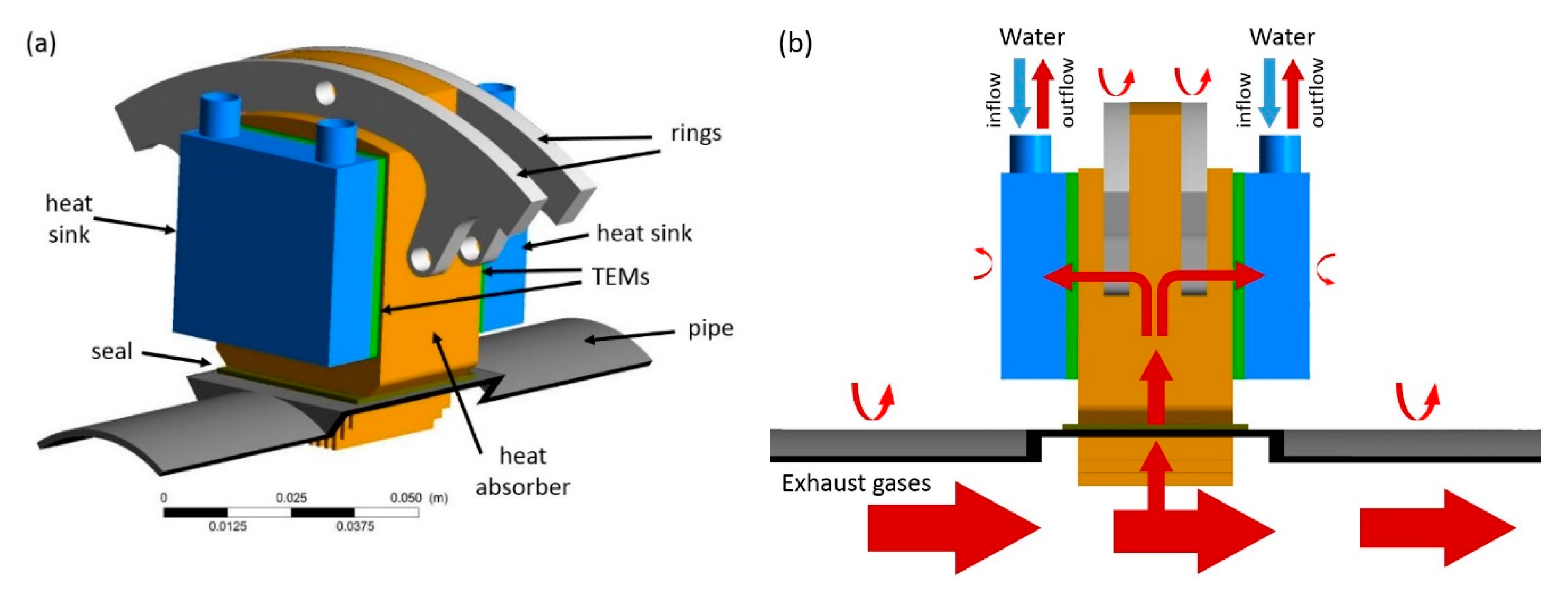
2.1. Radial ATEG

The radial ATEG mounts five identical cooling-TEM-heat absorber units (see Figure 1). The core of each unit is the heat absorber. It is made of a single block of copper with 15 precision machined fins at one end (Figure 1a). These fins are 1 mm thick and 30 mm long. The fin height is 10 mm in all fins except in fins #1 and #15 (5 mm high) and #2 and #14 (7.5 mm high), in order to avoid interferences with neighbor units. The heat absorbers were custom made by a local machining company according to our requirements. These copper units are inserted in a pentagonal pipe after applying a sealant at its contact base (Figure 1b). The total system of five copper heat absorbers accounts for an exchange surface area with the exhaust gases equal to At,o = 418 cm2. Each one of the heat absorbers is milled to 0.5 mm depth in a 40 × 46 mm surface area in both upstream and downstream faces for housing low temperature thermoelectric modules (H-199-14-06-L2, Crystal LTD [20]). Thermal grease was applied at both hot and cold sides of the TEMs for improving the heat transfer. The cold side of each TEM was in contact with a 40 × 40 mm BXQINLENX water heat sink. Two aluminum rings clamped together the water heat sinks located at both opposite faces, finally exerting on the TEMs a pressure that was equal to 0.9 MPa (Figure 1c).
Due to water pump limitations, each row of five water heat sinks are hydraulically connected in series. All 10 TEMs are electrically connected in series, since this connection is expected to produce higher output power than either parallel or hybrid ones [21]. The total weight of the system, including the 50 mm diameter pipes at both ATEG inlet and outlet, is only 4.8 kg. In addition, the system was very compact, with an overall diameter of 20 cm (excluding water pipes) and a length of 20 cm.
In comparison with other ATEGs, this design has several advantages. First, all TEMs possess a very similar temperature difference, since all of them absorb energy at the same point. Small differences appear due to the hydraulic connection in series but, as will be observed next, these are of low relevance. Thus, the external electrical load resistance can be tuned to match the optimum value that is valid for all TEMs. Second, the use of high volume heat absorbers avoids the overheating of TEMs without using any mechanical system. This allows us to use economic, free-Pb, low temperature TEMs. At the same point, this implies a high heat capacity of the heat absorbers, preventing fast fluctuations from being obtained in the output power as the regime changes in transient cycles. Finally, the radial distribution facilitates the individual monitoring of TEMs and their removal in case of malfunction.

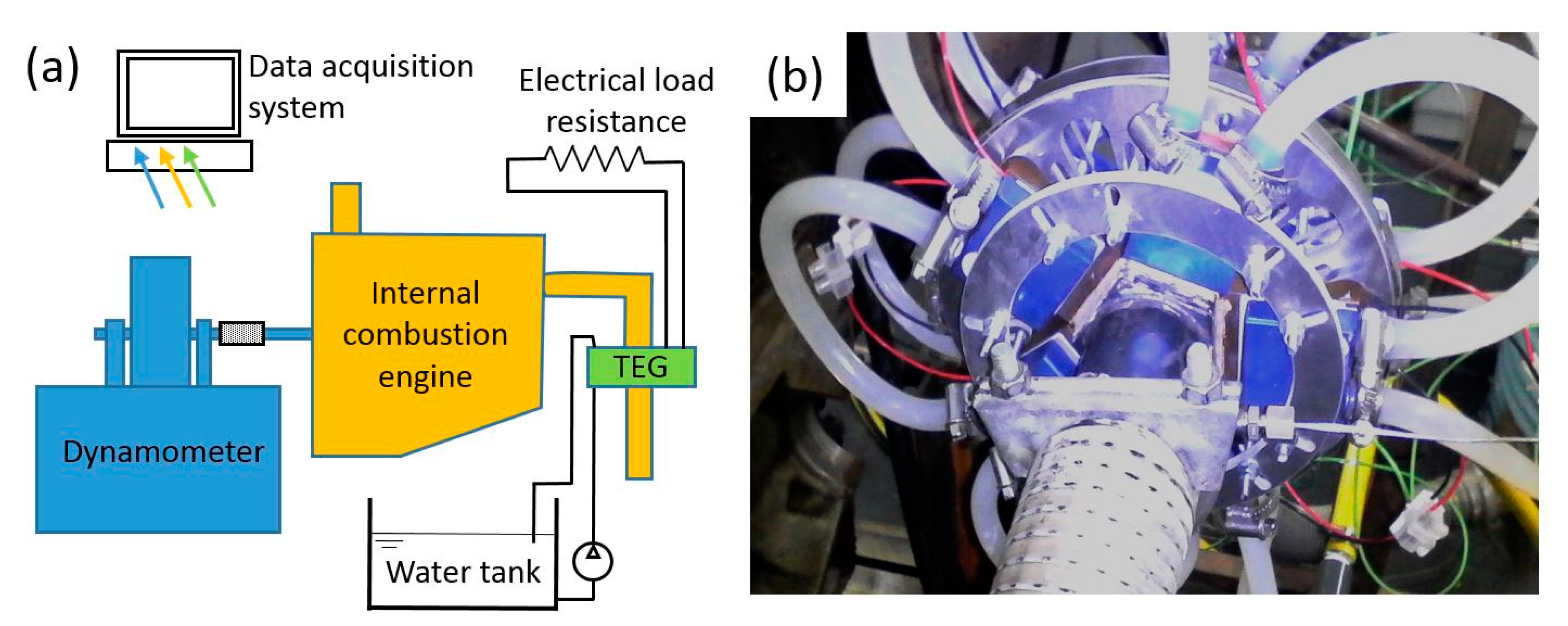
2.2. Experimental Set Up

The engine test bench uses a PSA XUD7 1.8 L diesel engine connected to a Schenck W130 dynamometer (Figure 2). Water initially at 19 °C from an external reservoir of 400 L capacity was used for cooling the ATEG. The flow rate was 4.4 liters/minute per each row of five water heat sinks that were hydraulically connected in series. In an ICE, the engine coolant temperature under regular functioning is in the order of 80 °C. This implies that our testing conditions were equivalent to include an independent cooling system for the ATEG in the case of being installed in a road vehicle. This strategy may be more suitable than redesigning the engine cooling system (radiator and pump) in order to operate with engine coolant, since the use of low temperature coolant for the heat sinks located at TEMs cold side is expected to substantially increase the electrical output power [22]. As already commented, the TEMs are electrically connected in series with a variable external load resistance.
Data from the dynamometer, ICE, and ATEG were simultaneously recorded. Exhaust gas temperatures at the ATEG inlet and outlet, the cold and hot side temperatures of TEM #1 (at water inlet) and #5 (at water outlet), the water temperatures at the ATEG inlet and outlet, and the ambient temperature were acquired with type K thermocouples by a National Instruments (NI) Compact RIO system with 9211 modules. In the electrical circuit, voltage and current were acquired by a NI Compact RIO with 9215 and 9227 modules. These data were processed with LabVIEW software.
The treatment of the experimental uncertainty and the accuracy of the equipment used in the experimental tests are described in detail in [21], where a similar laboratory layout was applied in the study of an ATEG with a single TEM. As a summary, the total uncertainty was calculated from the uncertainty of the data series ε d s recorded by the data acquisition system:
  ε d s = ± z α / 2 σ N   ,  
where z α / 2 is the confidence range, σ is the standard deviation and N is the number of samples, and the uncertainty of the equipment ε e q :
  ε e q = | Y x | Δ x   ,  
where Y corresponds to the indirect value, x refers to the direct measured value, and Δ x is the accuracy of the equipment in the measurement of the x value. Table 2 lists the main Δ x values of our equipment.
Thus, the total uncertainty of data ε t o t a l follows:
  ε t o t a l = ε d s 2 + ε e q 2   .  

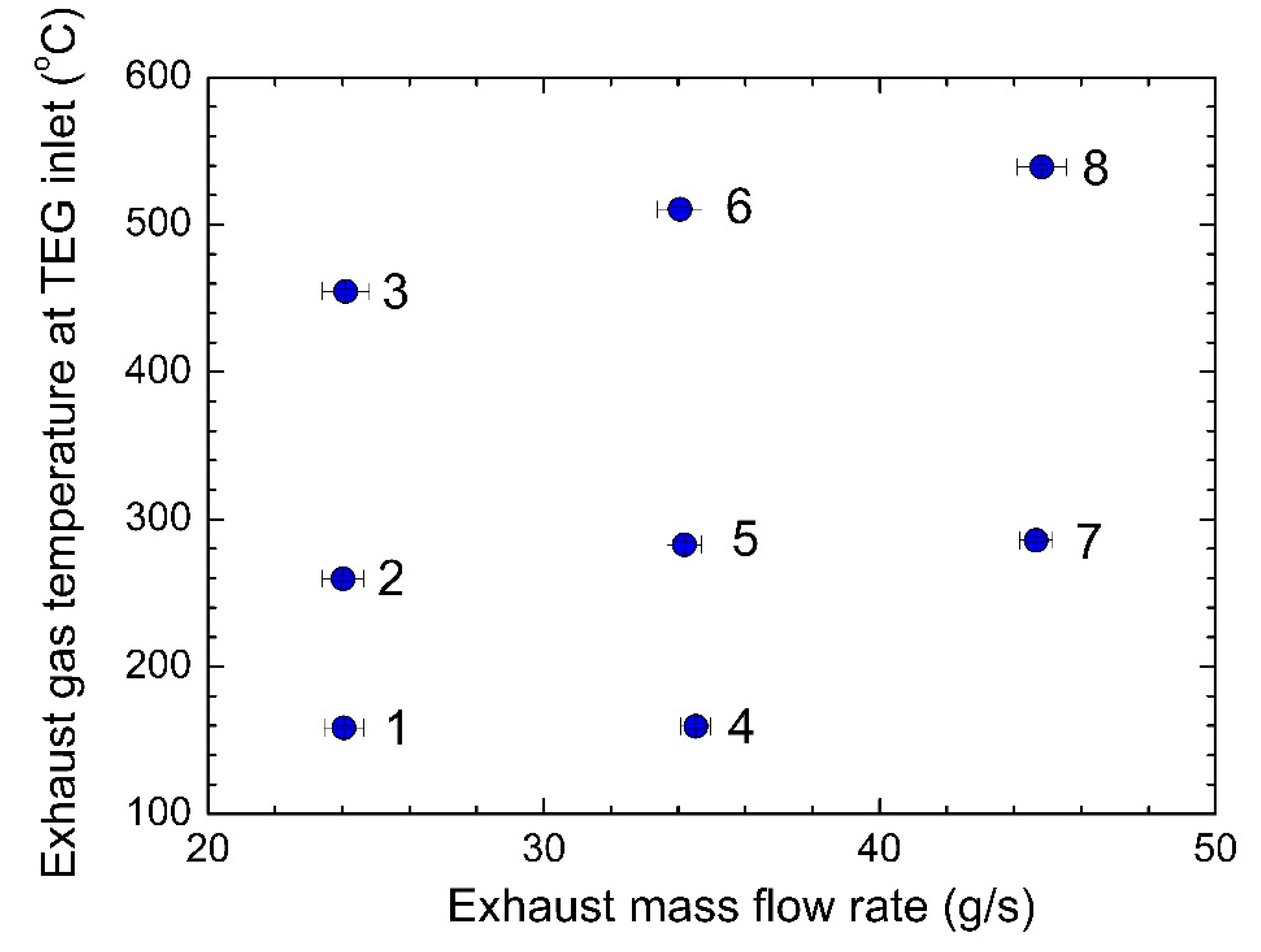
2.3. Experimental Cases

Eight different engine operating points were tested (see Figure 3). These points cover a broad working zone. Points 1 to 3 corresponded to scenarios at three different loads at a turning velocity equal to 1500 rpm; points 4 to 6 at a turning velocity of 2000 rpm, and points 7 and 8 at a turning velocity of 2500 rpm. Note that the exhaust mass flow rate was almost constant in points with equal turning velocity (see Table 3). In terms of load, almost no-load conditions were applied in points 1 and 4. An intermediate load were applied in points 2, 5 and 7, and a heavy load in points 3, 6 and 8. The temperature of the exhaust gases at the ATEG inlet was basically a function of the load applied to the engine. For each one of the eight different regimes, the external electrical resistance was tuned to achieve the maximum output power.

3. Numerical Model

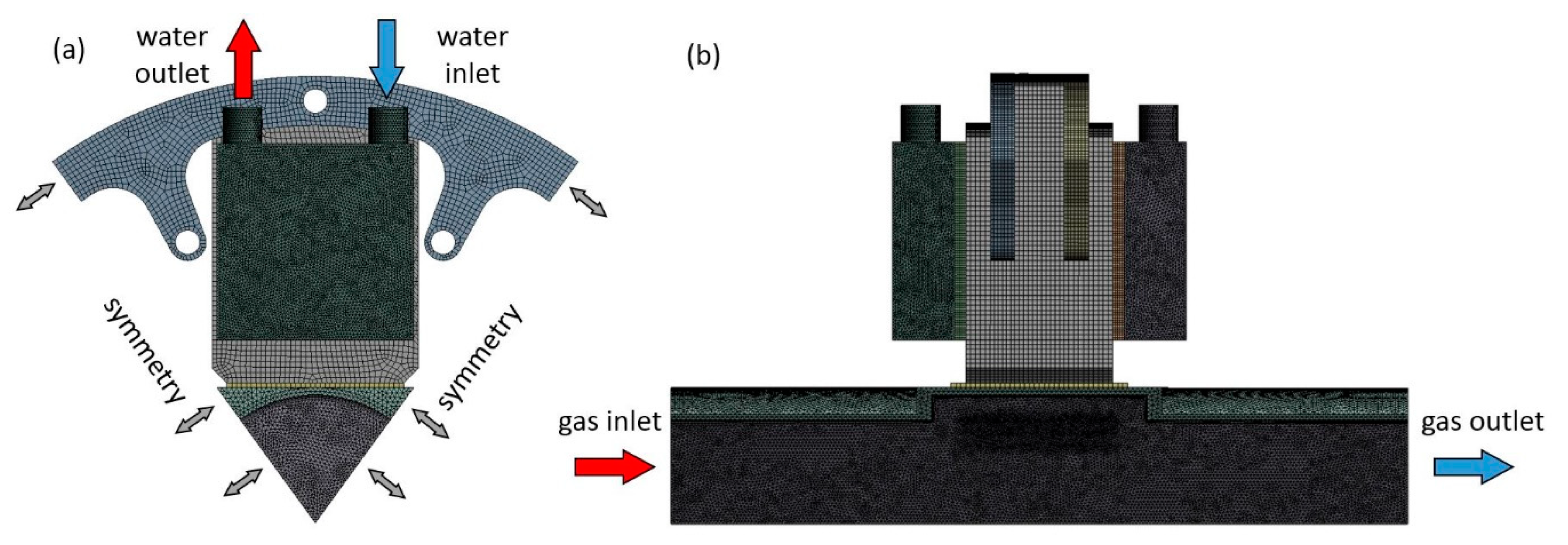
3.1. Simulation Set Up

A numerical model is developed in order to provide results when some of the design parameters of the radial ATEG are changed. The simulation technique reduced costs and time in the analysis of alternative designs, and it allowed us to carry out sensitivity studies to variations in the main properties of the ATEG elements. The commercial computational fluid dynamics (CFD) software ANSYS-CFX® was used, since it has the capability to correctly simulate the heat transfer between fluid flows and solid parts. Several researchers have applied this software to successfully predict heat transfer problems involving both fluid and solids (e.g., [26]).
The computational domain consisted of one-fifth of the whole radial ATEG, since it takes advantage of radial symmetry conditions (Figure 4). Six solids and two fluids were involved in the simulation. For the sake of simplicity, Figure 4a shows the solid elements only, namely: the heat absorber (copper), pipe (steel), seal (aluminum), two identical heat sinks (aluminum), two identical rings (aluminum), and two TEMs. The fluids were liquid water that flowed in the heat sinks and air (ideal gas law) that simulated the exhaust gases. The latter approximation is common in studies of ATEGs (e.g., [27]), since it is known to produce small discrepancies in comparison with the real exhaust flow behavior. A schematic drawing of the main heat flow path is shown in Figure 4b, where we included both the conduction and convection processes.
The actual radial ATEG tested in the engine bench did not strictly possess a radial symmetry, since rows of five water heat sinks (all upstream and all downstream ones) were connected in series due to water pump limitations. However, the experimental values of both hot and cold side temperatures at the first and last (#5) TEMs were very similar (see Section 3.2), which confirmed the validity of simulating one-fifth of the entire device only. On the other hand, the longitudinal dimension of the domain was chosen so as to reproduce the experimental ATEG from the position of the inlet temperature sensor to the position of the outlet temperature sensor (Figure 1 and Figure 2). Simulations with a pipe that was 50 mm longer at the exit have been also carried out. In the latter model, hot and cold side TEM temperatures and pressure changes across the ATEG differed less than 0.7% and 0.3%, respectively, in comparison with the results of the reference case. Therefore, the conclusions were expected to be independent of the simulation domain.
The mesh was created with ANSYS-Meshing®. Quadrilaterals with 1 mm maximum length were used to mesh the heat absorber, rings, and seal. TEMs were meshed with quadrilaterals of 0.5 mm maximum length. Tetrahedrons were used to mesh complex geometries such as the pipe (1 mm maximum length) and, especially, the heat sinks (0.6 mm maximum length), since they contained five small inner passages. Fluids were also meshed with tetrahedrons of 0.5 mm maximum length for water, and of 0.7 mm maximum length for the exhaust gas. In the latter case, a refiner mesh near the fins of the heat absorber was defined (0.2 mm maximum length). Four layers of prisms were created in contact with the solid surface (Figure 5). A total number of 8.8 × 10⁶ elements were needed to mesh all the domains, with 6.5 × 10⁶ elements dedicated to the gas subdomain. The maximum skewness and aspect ratio values were 0.89 and 23.3, respectively. This was equivalent to 44 × 106 elements for the entire ATEG device. Several coarser meshes were also simulated to evaluate the sensitivity of the results to changes in the mesh, as explained in Section 3.2. The finer mesh provided a wall-normal resolution y+ less than 5 (<15 for the coarser mesh), which agreed with the criterion employed in [12].
Boundary conditions fixed the values of mass flow and temperature at both gas and water inlet surfaces. These values corresponded to the experimental data obtained in the previous section. Constant pressure was set at both the water and gas outlets. All other boundaries were defined as either symmetrical or smooth walls. Heat transfer was allowed in all surfaces (see Figure 4b). Contact thermal resistances Rc were added between the heat absorber and the TEM hot side, and between the TEM cold side and the heat sink. A constant value of Rc = 10−4 m2 K W−1 was assumed, since it was representative of solid/solid interfaces [28] and similar values have satisfactorily been used in other studies of ATEGs [7]. Convection to the ambient air was allowed in all bodies, using a convective heat transfer coefficient for natural convection hc = 2 W m−2 K−1 [28]. The effect of including radiative fluxes in the simulation was analyzed, and it produces modifications in hot and cold side TEM temperatures less than 1%. Therefore, radiation was ignored since it substantially slowed down the calculation time and its inclusion did not alter the main conclusions of our research.
Heat transfer by conduction uses the thermal conductivity of solid and fluid elements. Here, each one of the TEMs was included as a single solid, so that effective thermal and electrical properties for the whole module were used. The effective thermal conductivity of the whole TEM was used in order to correctly capture the thermal behavior of the ATEG in the simulation process. The effective thermoelectric properties of the whole TEM (essentially the effective Seebeck coefficient) were not included in the simulations. This property was used in the analytical calculation of the maximum output power that the ATEG design could provide. This is a common strategy that is adopted to numerically analyze the behavior of large scale ATEGs [11,12,21]. Note that each individual TEM is formed by hundredths of p-type and n-type semiconductors that are connected in series with small sheets of copper that act as junctions of two dissimilar thermoelements and that are packed with two electrically isolating ceramic plates. The simulation of a single TEM taking into account all of these components would involve domains with characteristic sizes that differ in more than three orders of magnitude, and therefore, it would require very high computational resources.
Here, the effective thermal conductivity of the whole TEM ke, has been extracted by using the manufacturer’s datasheet of output power that is generated at a matched electrical load, expressing it as a function of temperature differences at both hot T h and cold T c sides of the TEM ( Δ T = T h T c ), being k e = 1.455 × 10 4 Δ T 2 + 0.0674 Δ T + 0.0269 .
Both exhaust gases and cooling water flow regimes are turbulent. The RNG k-ε turbulence model with 10% turbulence intensity at the inlet of exhaust gases and 5% turbulence intensity at water inlets has been adopted. High resolution schemes for both advection and turbulence are chosen, with a convergence criterion of RMS residuals of less than 10−5.
The previous set up of the CFD model simulates heat transfer and flow behaviors only. Electrical output power PATEG of the ATEG is calculated by assuming optimum conditions:
  P A T E G = n α e 2 Δ T 2 4 R i   ,  
where n (=10) is the number of TEMs, α e is the effective Seebeck coefficient, and Ri corresponds to the electrical load resistance that, per unit TEM, maximizes the output power. In Equation (4), we implicitly assume small variations among the Δ T measured in each individual TEM, since they are thermally connected in parallel. Due to the series connection of the water cooling system in the experimental study, there exist some deviations in the individual values of Δ T , although these are smaller than 5% for all regimes. On the other hand, the effective Seebeck coefficient α e employed in the calculation of the output power is chosen to match the experimental value determined from Equation (4). Thus, measured TEM hot and cold side temperature differences Δ T , electrical load resistance Ri, and output power P from the eight experimental cases detailed in Table 3 when substituted into Equation (4) provide values of the effective Seebeck coefficient. The mean value of these experimentally found effective Seebeck coefficients is α e = 0.052 V K−1 with a standard deviation equal to 0.003 V K−1.
The conversion of simulated ΔT into the power generated by the ATEG applies Equation (4) with a TEM-effective Seebeck coefficient that is equal to the mean value experimentally estimated from laboratory data ( α e = 0.052 V K−1) and an internal resistance per TEM that is equal to the value at nominal conditions indicated by the manufacturer (Ri = 1.86 Ω). This value agrees with the average external resistance Rexp (divided by the number of TEMs of the ATEG) that is experimentally obtained when it is tuned to achieve the maximum output power in the engine bench (the average value for all eight experimental cases is Rexp = 1.96 Ω with a standard deviation of 0.20 Ω). Indeed, both the effective Seebeck coefficient and the TEM internal resistance are slightly temperature-dependent within the temperature range that is observed in cases 1 to 8. However, we applied constant values of α e and Ri in Equation (4), since these temperature dependences were not provided by the manufacturer, and as in other studies with similar temperature ranges, they are expected to have little effect on the results (see, e.g., [12]). In our comparative analyses, this assumption did not invalidate the conclusions.

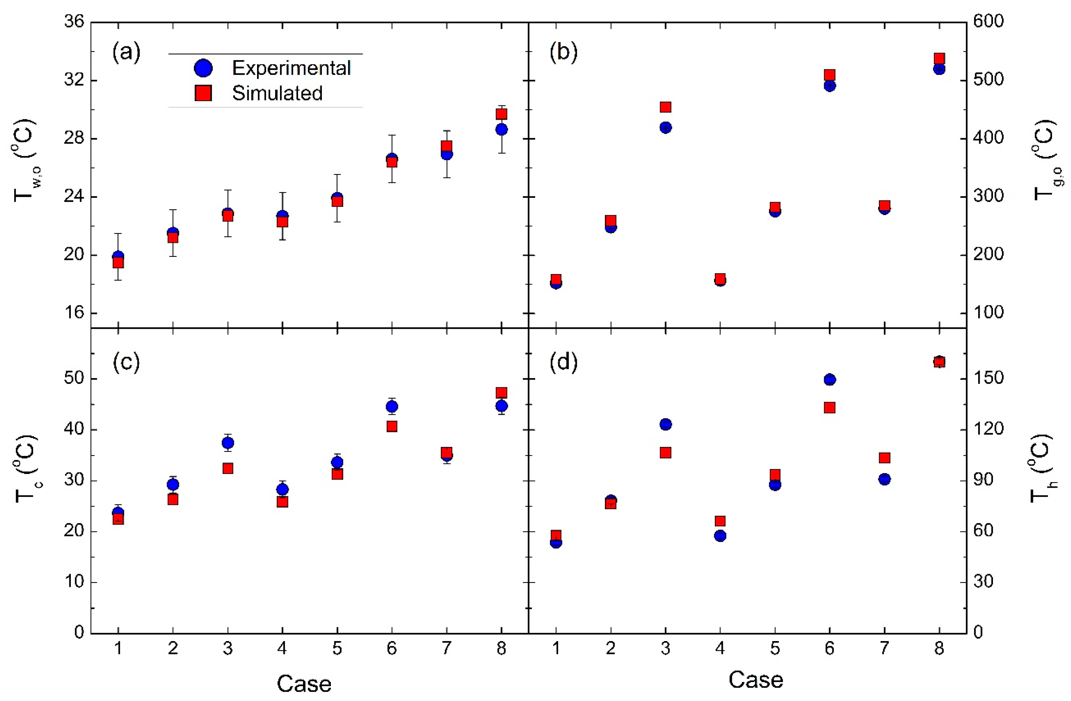
3.2. Model Validation

Experimental points 1 to 9 (Figure 3) were simulated with a set up that applies the boundary conditions detailed in Table 3. For fluids flows, the output results to compare with laboratory data were temperatures of exhaust gases at the ATEG outlet (Tg,o) and of the water coolant at the ATEG outlet (Tw,o). Since we studied one-fifth of the radial ATEG, the simulated value of Tw,o was multiplied by five in order to properly perform the comparison with measurements. For the solid bodies, temperatures predicted at both TEMs hot (Th) and cold (Tc) sides were compared with the experimental data (Figure 6).
From Figure 6, we observed that temperatures of both water and exhaust gases were very well reproduced by the model. It was very remarkable that the agreement of these temperatures was reached under very different engine operating points (ranging from low rpm at almost no load to high rpm and very high loads). On the other hand, hot and cold side TEM temperatures were also very well predicted in most of the cases.
Figure 7 compares the electrical output parameters calculated from simulations with those obtained experimentally. Note that the voltage and current obtained from the numerical model correctly reproduced the laboratory data, with a maximum in voltage and current for Case 8. This corresponds to the point with maximum turning velocity and engine load (Table 3), implying a very high temperature of the exhaust gases (Figure 6). In this case, the experimental output power obtained was 40 W at a TEM hot side temperature equal to 158 °C, and at TEM cold side temperature 46 °C. These temperature conditions almost coincided with the optimum performance point exposed in the manufacturer’s datasheet (Th = 150 °C, ΔT = 100 °C), from which an output power production of 10.9 W per module was expected at the matched resistance load. However, the laboratory data produced 4 W per module only. The reason for such a discrepancy on the TEMs performance could not be attributed to a mismatch in the working conditions of the modules, since TEM #1 (located at coolant inlet) is at Th = 160 °C and ΔT = 115 °C and TEM #5 (located at coolant outlet) is at Th = 155 °C and ΔT = 108 °C. The small difference in the TEM working conditions could not be responsible for reducing the expected power by more than half. In addition, the external resistance was tuned to reach the maximum output power during each stationary regime. The difference may be a consequence of the clamping force that was set to be equal to 1500 N per module, equivalent to a pressure of 0.9 MPa. This conservative value was chosen in order to prevent cracks in the module, especially in the zone that was free of semiconductor pellets where the electrical wires were soldered. This was observed to be the most fragile region of the TEM, since the inlet and outlet hoses of the individual water cooling pressed on it once we had assembled the ATEG. At higher loads (2000 N, as recommended in 40 × 40 mm TEMs by some manufacturers), some of the TEMs cracked and they had to be replaced, and the ATEG reassembled with a more conservative clamping load. However, this did not affect the validation procedure, since numerical calculations of the output power applied an effective Seebeck coefficient that was extracted from the experimental data.
We also carried out a grid independence study. The results shown here corresponded to the finer mesh (8.8 × 10⁶ elements). However, simulations with coarser grids (6.4 × 10⁶, 5.1 × 10⁶, 4.2 × 10⁶, and 3.7 × 10⁶ elements) have been obtained. This has allowed us to calculate the Grid Convergence Index GCIfine21 for the main variables in the system by applying the methodology detailed in [29]. In a numerical simulation of fluid flows, the GCIfine21 index is accepted as an indicator of the discretization error. The mesh independency study gave: GCIfine21 = 2.7% (order p = 0.4) for Th, GCIfine21 = 6.7% (order p = 1.0) for Tc, and GCIfine21 = 1.2% (order p = 3.4) for Δpdp.
From the above, and since the output power simulated for all cases agreed with laboratory data within the uncertainty range of the experiment (Figure 7), we accepted that the model was suitable to carry out comparative analyses of the ATEG performance when some of its design parameters were changed, as in Section 4.

4. Results and Discussion

The continuous research for developing ATEGs faces two challenging tasks: (1) the design of heat exchangers that increase the heat transfer without penalizing the fuel consumption, and (2) the improvement of the heat-to−electricity conversion rate of thermoelectric materials. Here, we analyzed the effects of modifying both the heat exchanger and the efficiency of the thermoelectric modules.
Each one of the five heat absorbers that form the ATEG tested in the engine bench used straight fins that were 1 mm wide with a total surface area At,o = 418 cm2 (Figure 1). In the present comparative analysis, we increased the surface area of the heat absorber by increasing the height of the fins while maintaining the width (=1 mm) and the fin-to-fin distance (=1 mm). Figure 8 shows the four cases analyzed that correspond to heat absorbers with an effective increase in the surface area of the heat absorber equal to 20%, 40%, and 60% with respect to At,o.
On the other hand, the effective figure of merit Z T e of the TEM module was calculated with the following equation:
  Z T e = α e 2 T ¯ ρ e k e   ,  
where T ¯ is the average temperature of Th and Tc, and ρ e is the TEM-effective electrical resistivity, with all previous data calculated at nominal conditions. Following the manufacturer’s datasheet, at nominal conditions, T ¯ = 373.15 K, ρ e = 0.902 Ωm, k e = 5.33 W K−1 m−1 and α e = 0.090 V K−1. This gives a value of the effective figure of merit Z T e = 0.63 . However, under laboratory conditions, the actual effective Seebeck coefficient is α e = 0.052 V K−1, as already discussed at the end of Section 3.1. In this case, the effective figure of merit of the TEMs, once installed in our ATEG, was Z T e = 0.21 only, being three times smaller than the expected value. Since we applied the effective value of the Seebeck coefficient extracted from the laboratory data in order to convert heat into electricity, the power generated was also three times lower than expected.
In the following subsections, a comparative analysis of the effect of using different heat absorbers on the electrical power output, as well as on the fuel economy, was carried out by means of the numerical model.

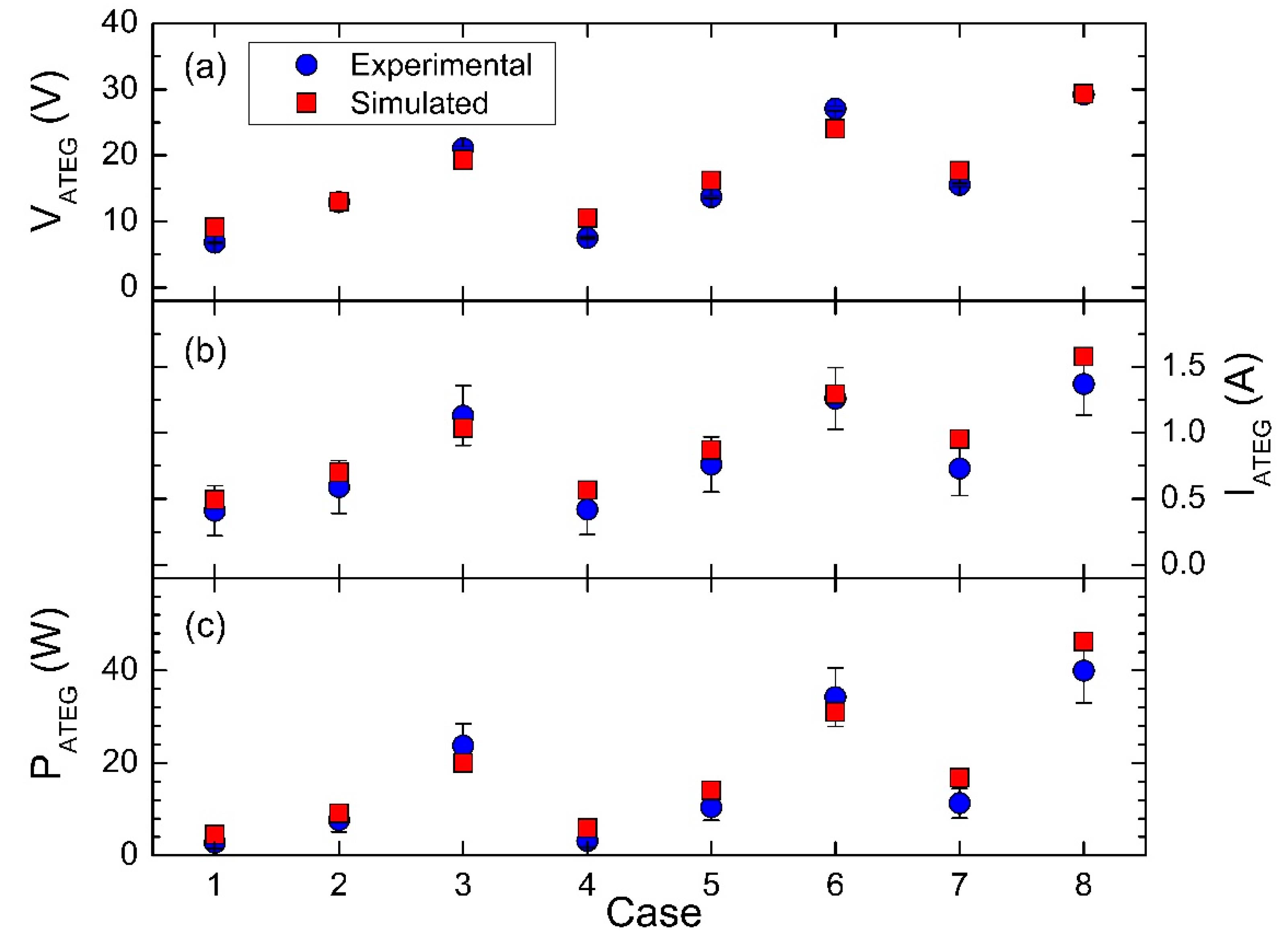
4.1. Electrical Power Output
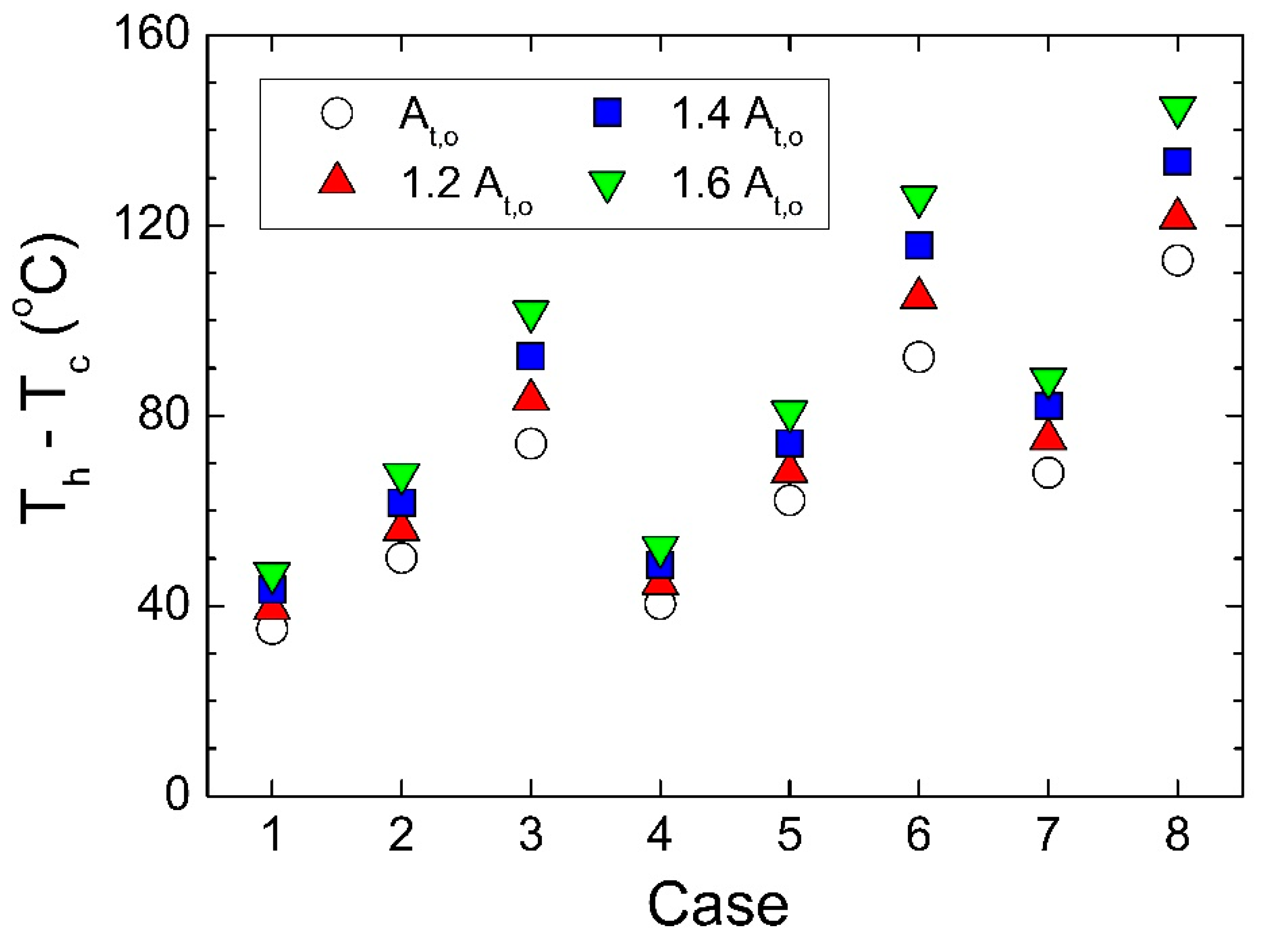
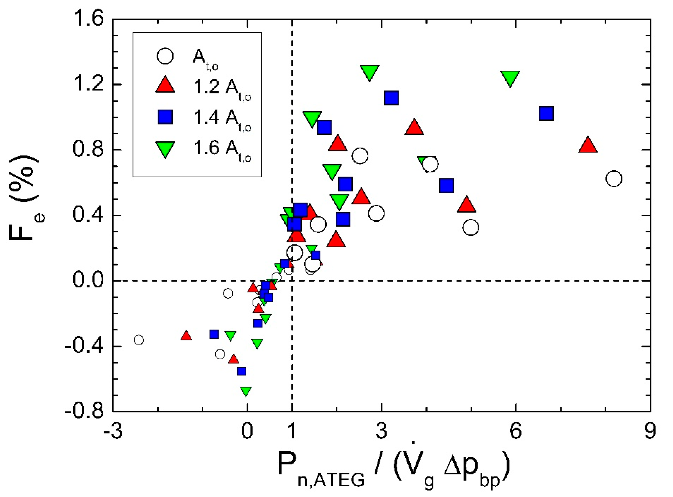
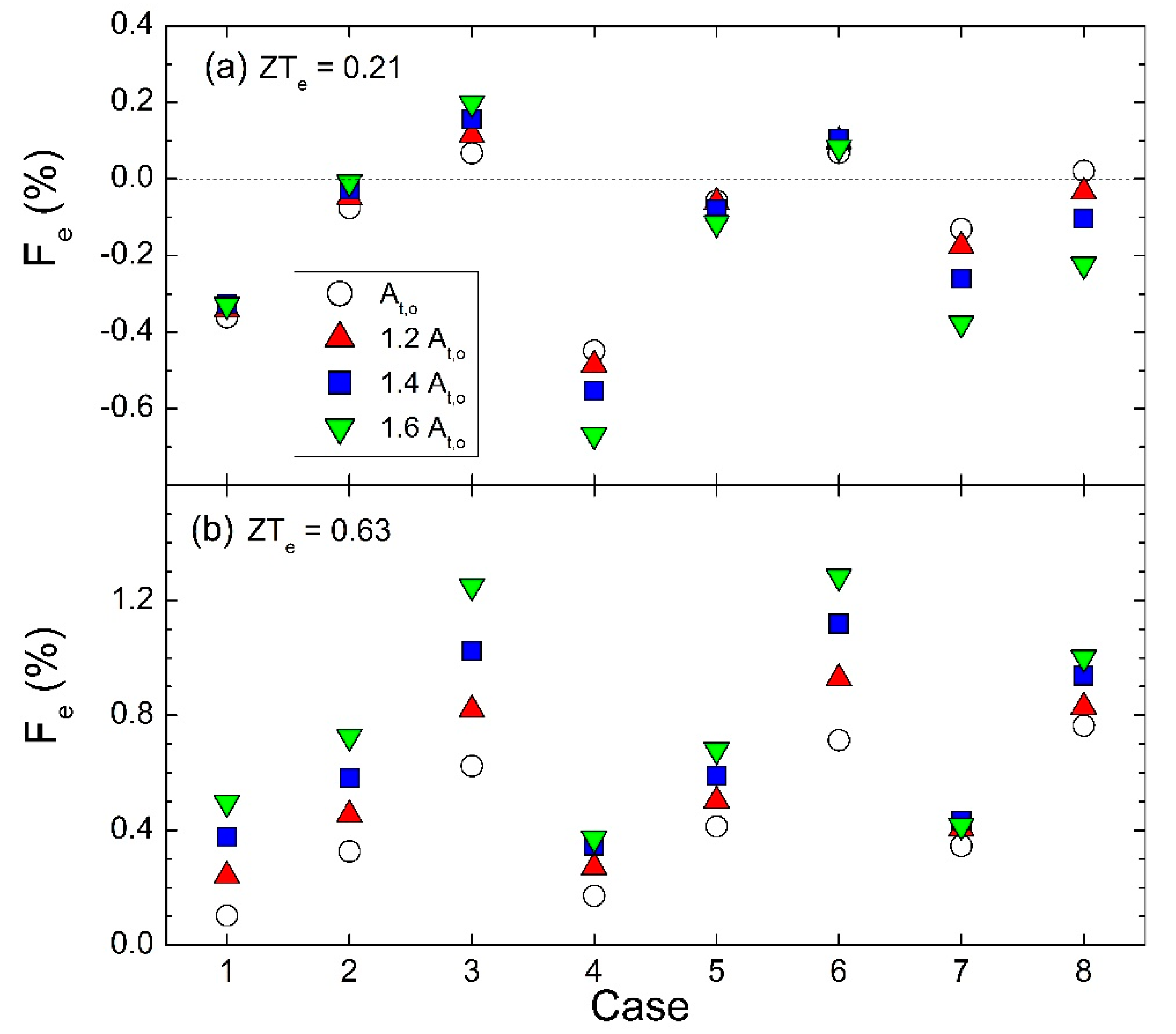
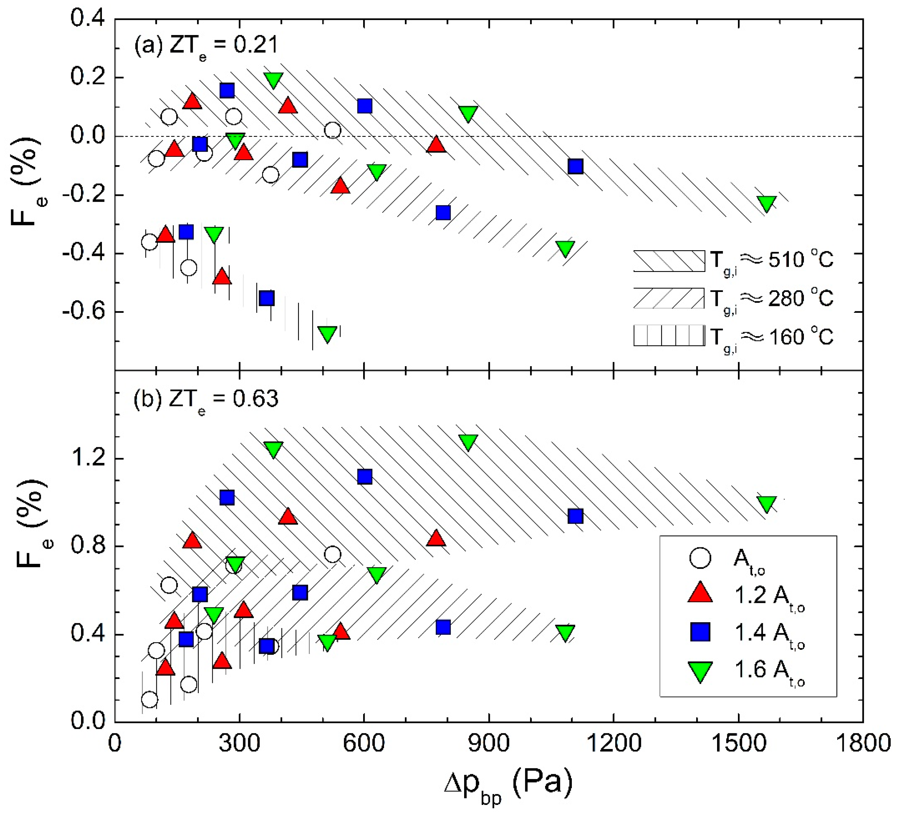
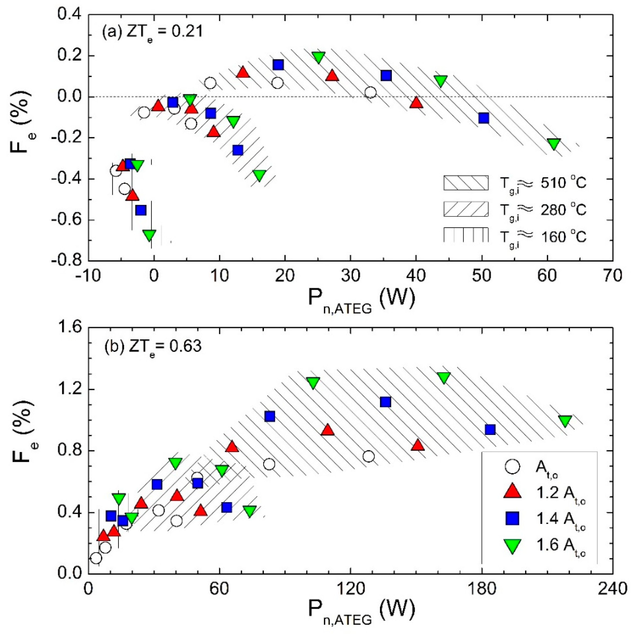
Temperature differences between both the hot and cold sides of the TEM obtained when using heat absorbers with different total surface areas for each one of the cases studied in Figure 3 are shown in Figure 9. The average increase in ΔT = ThTc with respect to the reference design (heat absorber with total surface area equal to At,o) was 11%, 22%, and 33% when increasing the total fin surface area by 20%, 40%, and 60%, respectively. The maximum increase in ΔT is observed in case 3, being 13%, 25%, and 37% corresponding to heat absorbers with 20%, 40%, and 60% more total fin surface area than that of the reference design. In general, the increase in the total surface area of the heat exchange zone with the exhaust gases favored the raise of ΔT in those engine regimes with low mass flow rates (cases 1, 2, and 3 in Figure 3). In comparison, the gain in ΔT at high regimes (e.g., cases 7 and 8) was proportionally, not as pronounced.
Figure 10 shows the temperature variations that occurred in the heat absorber when changing the fin dimensions in case 8. The ATEG with heat absorbers with very high fins (Figure 10b) almost completely blocked the incoming flow that was forced to go through the fin exchanger. This substantially increased the temperature of the fins in comparison with the design tested in Section 2 (Figure 10a). Under the same incoming flow, temperatures may be higher than 100 °C of those found in the original design. This finally led to an increase in the temperature of the body of the heat absorber, and hence, a greater ΔT of the TEM. Note that simulations clearly predicted a reduction of the heat absorber temperature from fins to the body, and even there, the temperature decays as it approaches the outer rings. This was a consequence of heat losses to the ambient surroundings, as well as to the heat flow through the different solid elements until reaching the water heat sinks located at the cold side of the TEMs. Note that although fin temperature was clearly higher in the upstream region, the high thermal conductivity of copper led to almost equal average temperatures in the hot side faces of both upstream and downstream TEMs (variations of less than 0.5 °C).
The maximum electrical output power PATEG per each case of Figure 9 is depicted in Figure 11. Since PATEG is proportional to ΔT2, the average increase in PATEG with reference to the initial design tested in the engine bench (Section 2) was 23%, 49%, and 75% when the total fin surface area of the absorber increased by 20%, 40%, and 60%, respectively. In case 8, the maximum output power for the 1.6At,o heat absorber type reached 76 W, in comparison with the 46 W obtained with the At,o case. In case of using the modules with ZTe = 0.63, the output power would rise up to 228 W and 138 W, respectively.
The efficiency ηTEM of the heat to electricity conversion can be calculated from the electrical output power of a single TEM PTEM (=PATEG/10) and the heat flow through its hot side Qh:
η T E M   ( % ) = 100 P T E M Q h   .  
Under engine operating conditions equal to case 1, the heat flow of the original design is Qh = 34.5 W, leading to a TEM efficiency of η T E M = 1.3%. This value increases up to η T E M = 1.9% under conditions of case 8 (Figure 10a), where the heat flow increases up to Qh = 242 W. The modification of the heat absorber including higher fins, did not substantially increase the TEM efficiency. In the 1.6At,o total surface area design, and for cases 1 and 8 (Figure 10b), the heat flow was Qh = 58 W and Qh = 377 W, respectively, increasing the efficiency by only 0.1%, in comparison with the original design. Thus, a maximum of η T E M = 2.0% was obtained, which was slightly below the values claimed by other authors in the study of ATEGs (on the order of 2.6% [9,13]). An increase in the ZTe value up to 0.63, according with our TEMs datasheet, would imply TEM efficiencies on the order of 6.0% maximum.
The reduction of the available cross-sectional area for the exhaust flow implied an increase in the energy losses along the exhaust pipe. This phenomenon was equivalent to enhancing the value of the required pressure upstream the pipe in order to properly drive the flow to the exit (at atmospheric pressure). We defined the back pressure Δpbp as the pressure change between both the inlet and outlet cross-sections of the ATEG. An increase in the back pressure may have adverse consequences on the regular functioning of the engine, leading to an increase in the fuel consumption. Therefore, not only output power, but also back pressure values are worthy of investigation when developing ATEG designs.
Figure 12 shows the value of the back pressure Δpbp for all of the eight cases tested in the laboratory. As expected, Δpbp increased as a function of the mass flow rate in those cases with almost equal gas inlet temperatures. On the other hand, Δpbp increased as a function of the gas inlet temperature when the mass flow rate was kept constant. The effect of enlarging the total surface area of fins At of the heat absorber dramatically increased the energy losses. An average of a 45%, 108%, and 192% increase in Δpbp with respect to the At,o case was observed for those designs with At = 1.2 At,o, 1.4 At,o, and 1.6At,o respectively.
It is very remarkable that, for a fixed exhaust gas temperature, the electrical output power could be directly related with the back pressure values for any of the designs proposed (Figure 13). This general behavior of our radial design would allow us to predict the output power once the value of the energy losses through the exhaust was estimated. This would be a very fast method to assess the potential of electrical generation of the ATEG without the need to carry out either complex simulations or experimental tests. We point out that a similar behavior has been recently observed in an ATEG with circular tubes as heat absorbers [30], being used for developing an analytical method to calculate the fuel economy.
Power production may be enhanced by adding another radial ATEG in series configuration. We numerically analyzed this case under conditions of case 8 with the original configuration of the heat absorber. Since the temperature of the exhaust gases at the output of the first radial ATEG decreased, the power of the second radial ATEG reached only 27 W, in comparison with the 46 W obtained in the upstream one. Therefore, the strategy of adding more and more TEMs in an ATEG with the purpose of increasing the output power may clearly fail, since the geometrical distribution of TEMs to maximize the available waste heat is a key factor of the ATEG performance [21].

4.2. Fuel Economy

The electrical output power generated by an ATEG is useful information for deciding whether or not the design has the potential to supply a reasonable amount of power to the vehicle. Nevertheless, it is worth mentioning that the ultimate goal of an ATEG is to reduce the fuel consumption rather to maximize power. Previous experimental studies on ATEGs provide data of electrical output power, since it is a straightforward measure. However, very few evaluate the implications on the fuel consumption. This is due to the fact that the conversion of power output to fuel savings is a very complex task where a myriad of factors may be relevant.
Here, we numerically estimate the impact of the ATEG on fuel consumption following the methodology developed by Karri et al. [31]. For simplicity, we account for only two terms, the contribution to the fuel economy due to (1), the power generated by the ATEG ( F e , A T E G ), and (2) the power required to overcome the back pressure that is generated by the ATEG ( F e , B P ):
F e , A T E G ( % ) = 100 η P C U η G   P e P n , A T E G   ,
  F e , B P ( % ) = 100 V ˙ g Δ p b p P e     ,  
where η P C U (=0.84 [30]) is the efficiency of the power converter unit (PCU), which is a direct-current to direct-current converter to match the output voltage of the electrical generator of the vehicle, η G (=0.5 [30]) is the efficiency of the mechanical to electrical conversion of the electrical generator of the vehicle, P e is the engine shaft power (equal to the torque multiplied by the turning velocity of Table 3, and assumed not to vary for each single case when using different ATEG designs), P n , A T E G is the net power produced by the ATEG (ATEG generation minus the power required for pumping the water in the ATEG cooling system), and V ˙ g is the volumetric flow rate of exhaust gases. Note that F e , B P is a negative contribution to fuel economy, as expected. The value of P n , A T E G is here calculated as P n , A T E G = P A T E G P w p where P w p is the power that is required by the water pump installed at the cooling system of the ATEG (see Figure 2a). In our experiment, we used a large reservoir for the cooling system so that the pumping power that was required simply reduced to the value needed to drive the water through water pipes and heat sinks. CFD simulations gave a pressure loss that was equal to 3.1 kPa (pressure difference between the exit and the inlet of the water heat sink). Since we have five heat sinks in a series configuration, and a constant volumetric flow rate of 4.4 liters/minute for all cases, the pumping power would be on the order of 1.2 W only. To this value, we must add the pumping power that is required to drive water through the cooling lines of the ATEG. For all cases, we have assumed a conservative value of P w p   = 10 W, which agrees with the coolant pumping power that is proposed in [31] for a similar flow rate.
Thus, the fuel economy F e   is calculated as:
  F e = F e , A T E G + F e , B P   .  
We stress that Equation (9) gives the maximum possible value of fuel economy assigned to the ATEG device, since P n , A T E G , as calculated in Equation (4), corresponds to the maximum power value, and Equation (9) neglects any additional terms that tend to reduce the fuel economy, such as the increase of power that is needed to transport the ATEG weight. The latter contribution was neglected, since it required the speed of the vehicle, and since our test was on an engine bench, this velocity should be estimated with the transmission ratio, axle ratio, tire diameter, transmission efficiency, etc., which are data from components that were not available in our laboratory. All in all, the Fe value here calculated must be understood as the maximum possible value of fuel economy that was achieved with our ATEG design.
Figure 14 shows F e   for all of the cases previously analyzed using TEMs with an effective figure of merit ZTe = 0.21 or ZTe = 0.63. Cases with ZTe = 0.21 and total fin surface area At = At,0 correspond to the laboratory conditions described in Section 2. In these cases, only three of the eight regimes provided fuel savings. However, these fuel economy values were so small that we could conclude that the original ATEG design did not contribute to improving the engine fuel consumption.
When increasing the total fin surface area, the back pressure effect was more adverse than in the base case. Thus, although electrical power increased, the overall contribution led to an increase of the fuel consumption for the 1.6At,o case, especially at high engine regimes and high engine loads. At low regimes, since the back pressure was not excessive, the 1.6At,o case gave slightly better results than the At,o case. In view of the fuel economy results, the overall conclusion was that the radial ATEG designs here proposed when using TEMs with ZTe = 0.21 were not feasible.
However, the improvement of the thermoelectric properties of the TEMs up to ZTe = 0.63 values under the same thermal properties as in those modules initially used, allowed positive fuel savings to be reached under all conditions (Figure 14b). The maximum fuel economy was achieved at intermediates regimes, since the high value of the back pressure strongly penalized the outcome under high regime conditions.
Results from Figure 14 confirmed that the condition of maximum fuel savings did not coincide with the maximum electrical output power. Therefore, studies on ATEGs should focus on how to improve fuel consumption, and not only on maximizing generated power. Besides power, key information such as back pressure values and, in non-stationary engines, the ATEG mass value, should be provided to estimate the impact of the ATEG on fuel economy.
In Figure 13, we clearly identified a common trend of generated power as a function of back pressure in the form P A T E G = a + b Δ p b p + c Δ p b p 2 , with a, b and c constants for a fixed value of the exhaust gas temperature at ATEG inlet. In terms of fuel economy, this unique dependency with the back pressure was not observed, as it can be seen in Figure 15. In this figure, different hatched areas correspond to cases with different exhaust gas temperatures at ATEG inlet. From Equations (7) and (8), fuel economy not only depends on Δ p b p but also on the volumetric flow rate of exhaust gases V ˙ g and on the engine shaft power P e . Both terms cannot be expressed as a function of Δ p b p only. Thus, F e / 100 = d ( a + b Δ p b p + c Δ p b p 2 P w p ) P e 1 V ˙ g Δ p b p P e 1 with d a constant. At low values of the figure of merit of the TEMs, the energy production was low, and in most of the cases, the dominant term was the negative contribution of the back pressure. As ZTe increased, the power generation term eventually led to positive fuel savings, reaching a maximum at intermediate back pressure conditions.
At low engine load regimes (exhaust gas temperature at ATEG inlet on the order of 160 °C), the output power generated (with ZTe = 0.21) was even lower than that required for pumping water in the ATEG cooling system. As a consequence, Pn,ATEG was negative (Figure 16). This led to an increase of the fuel consumption of almost 0.7% in the design that had a total fin surface area At = 1.6 At,0, since in this case, there was also a high penalization due to the back pressure value. The latter played a key role in the determination of fuel consumption, since even with ZTe = 0.63 (Figure 16b), the maximum fuel saving did not coincide with the maximum net output power, except for the original design due to the comparatively low Δpbp values reached.
ATEG designs able to generate the same output power but at lower engine loads substantially improved the fuel savings. When the figure of merit increased, the TEM power production enhanced, and larger differences of performance between designs were observed. For ZTe = 0.63, the maximum degree of fuel savings was equal to 1.3% at intermediate regimes and high load, whereas the maximum power was equal to 228 W at the highest engine regime and load in both cases for the ATEG design with the greatest surface area of the heat absorber-gas exchange (d in Figure 8). However this layout was the worst one at high engine regimes, in terms of fuel efficiency, when the TEM’s effective figure of merit ZTe = 0.21.
It would be of interest to have a simple rule-of-thumb to determine whether or not an ATEG design is feasible in terms of fuel consumption. From Equation (9), the ratio Fe,ATEG/Fe,BP P n , A T E G / ( V ˙ g Δ p b p ) , since η P C U / η G is on the order of 1. Thus, positive fuel savings are expected when Fe,ATEG/Fe,BP > 1 or, equivalently, P n , A T E G / ( V ˙ g Δ p b p ) > 1, as it is shown in Figure 17. The relevant point is that optimum conditions in terms of fuel economy are reached at intermediate values of P n , A T E G / ( V ˙ g Δ p b p ) (from 2 to 4 depending on the radial ATEG design). Note that points with maximum P n , A T E G / ( V ˙ g Δ p b p ) values correspond to those of the lower regime (1500 rpm), since V ˙ g Δ p b p takes low values. However, the reduction in fuel consumption when P n , A T E G / ( V ˙ g Δ p b p ) >>1 is not very high, since the electrical output power in these points is very modest.

5. Conclusions

We have designed a new type of ATEG with the purpose of using economic, lead-free, low-temperature commercial TEMs without adding any complex mechanical systems to regulate the flow of exhaust gases. A novel radial ATEG with 10 commercial TEMs has been built and tested in an engine bench under eight different engine operating conditions.
A numerical model based on commercial software ANSYS-CFX® has been developed, coupling fluid flows (exhaust gases and water cooling system) and solid bodies in the study of the heat transfer. This model has been validated with the experimental data obtained in the laboratory.
Several ATEG designs with different total surface area of exchange with the exhaust gases have been simulated. In addition, the effect of increasing the conversion rate of heat into electricity of the commercial modules has also been investigated. For all scenarios, values of electrical output power and fuel savings have been reported. Fuel savings values correspond to maximum figures due to the assumptions done in our calculations.
From our findings, we conclude that the electrical output power can be expressed as a parabolic function of the ATEG back pressure when working in conditions of equal exhaust gas temperature at the ATEG inlet. The maximum output power is reached at the highest engine regime with the highest engine load, since it implies conditions of maximum exhaust gas mass flow rate and exhaust gas temperature. However, even in these conditions, the temperature reached at the hot side of the TEM does not exceed its maximum operating temperature (200 °C), which assures the integrity of the system, even in the most demanding working regimes.
Results confirm that back pressure severely affects the fuel savings. This implies that the point of maximum electrical output power does not always coincide with that of maximum fuel economy. In our study, the maximum fuel economy for an effective figure of merit equal to that found in the experimental test, is reached at high engine loads but at low engine regimes. In addition, the strategy to increase the total surface area of the heat exchanger in contact with the exhaust gases may be counterproductive in some engine regimes, since the fuel consumption may greatly increase due to the increment in the back pressure. Thus, analyses of ATEGs should include not only studies on electrical output power, but also on fuel economy.
For a given ATEG configuration, there exists a threshold value of the effective figure of merit ZTe, beyond which all the regimes analyzed produce positive fuel savings. In our designs, a value of ZTe = 0.63 leads to a maximum reduction of fuel consumption of 1.3%, with an efficiency of TEM energy conversion that is equal to 6%.
Finally, we propose the dimensionless expression P n , A T E G / ( V ˙ g Δ p b p ) as a simple parameter to determine the feasibility of the ATEG design. Only those cases with P n , A T E G / ( V ˙ g Δ p b p ) > 1 may be of interest in terms of fuel consumption. In our radial ATEG, maximum efficiency values are achieved when P n , A T E G / ( V ˙ g Δ p b p ) ranges from 2 to 4. Although other types of ATEG designs may have their own maximum ranges, the P n , A T E G / ( V ˙ g Δ p b p ) > 1 criterion still holds.

Author Contributions

M.C. conducted the experimental study, including all the setup of the engine test bench. M.C., T.P., I.R.C., and A.M. conducted the detailed modeling and the validation study. M.C. and E.M. carried out the analyses of the results. M.C. and T.P. wrote the paper.

Funding

This work has been partially funded by the University of Girona under grant MPCUdG2016-4.

Acknowledgments

The authors gratefully acknowledge the technical support provided by Sergi Saus and Jordi Vicens. Iker Garcia provided very helpful assistance in the CAD/CFD drawings.

Conflicts of Interest

The authors declare no conflict of interest. The funders had no role in the design of the study; in the collection, analyses, or interpretation of data; in the writing of the manuscript, or in the decision to publish the results.

References

  1. The World Bank. Available online: https://data.worldbank.org/indicator/en.co2.tran.zs?end=2014&start=1960 (accessed on 5 September 2018).
  2. European Environment Agency. Available online: https://www.eea.europa.eu/data-and-maps/indicators/transport-emissons-of-greenhouse-gases/transport-emissions-of-greenhouse-gases-10 (accessed on 5 September 2018).
  3. European Comission. Available online: https://ec.europa.eu/clima/policies/transport_en (accessed on 5 September 2018).
  4. European Commission. Clean Power for Transport: A European Alternative Fuels Strategy. Communication from the Commission to the European Parliament, the Council, the European Economic and Social Committee and the Committee of the Regions; COM(2013) 17; European Commission: Brussels, Belgium, 2013. [Google Scholar]
  5. Rahman, A.; Razzak, F.; Afroz, R.; AKM, M.; Hawlader, M.N.A. Power generation from waste IC engines. Renew. Sustain. Energy Rev. 2015, 51, 382–395. [Google Scholar] [CrossRef]
  6. Karvonen, M.; Kapoor, R.; Uusitalo, A.; Ojanen, V. Technology competition in the internal combustion engine waste heat recovery: a patent landscape analysis. J. Clean. Prod. 2016, 112, 3735–3742. [Google Scholar] [CrossRef]
  7. Massaguer, A.; Massaguer, E.; Comamala, M.; Pujol, T.; Montoro, L.; Cardenas, M.D.; Carbonell, D.; Bueno, A.J. Transient behavior under a normalized driving cycle of an automotive thermoelectric generator. Appl. Energy 2017, 206, 1282–1296. [Google Scholar] [CrossRef]
  8. Frobenius, F.; Gaiser, G.; Rusche, U.; Weller, B. Thermoelectric generators for the integration into automotive exhaust systems for passenger cars and commercial vehicles. J. Electron. Mater. 2016, 45, 1433–1440. [Google Scholar] [CrossRef]
  9. Kim, T.Y.; Kwak, J.; Kim, B.W. Energy harvesting performance of hexagonal shaped thermoelectric generator for passenger vehicle applications: An experimental approach. Energy Convers. Manag. 2018, 160, 14–21. [Google Scholar] [CrossRef]
  10. Fernández-Yáñez, P.; Armas, O.; Kiwan, R.; Stefaopoulou, A.G.; Boehman, A.L. A thermoelectric generator in exhaust systems of spark-ignition and compression-ignition engines. A comparison with an electric turbo-generator. Appl. Energy 2018, 229, 80–87. [Google Scholar]
  11. Stobart, R.; Wijewardane, M.A.; Yang, Z. Comprehensive analysis of thermoelectric generation systems for automotive applications. Appl. Therm. Eng. 2017, 112, 1433–1444. [Google Scholar] [CrossRef]
  12. Wang, Y.; Li, S.; Xie, X.; Deng, Y.; Liu, X.; Su, C. Performance evaluation of an automotive thermoelectric generator with inserted fins or dimpled-surface hot heat exchanger. Appl. Energy 2018, 218, 391–401. [Google Scholar] [CrossRef]
  13. Orr, B.; Akbarzadeh, A.; Lappas, P. An exhaust heat recovery system utilizing thermoelectric generators and heat pipes. Appl. Therm. Eng. 2017, 126, 1185–1190. [Google Scholar] [CrossRef]
  14. Lan, S.; Yang, Z.; Chen, R.; Stobart, R. A dynamic model for thermoelectric generator applied to vehicle waste heat recovery. Appl. Energy 2018, 210, 327–338. [Google Scholar] [CrossRef]
  15. Crane, D.; Lagrandeur, J.; Jovovic, V.; Ranalli, M.; Adldinger, M.; Poliquin, E.; Dean, J.; Kossakovski, D.; Mazar, B.; Maranville, C. TEG on-vehicle performance and model validation and what it means for further TEG development. J. Electron. Mater. 2013, 42, 1582–1591. [Google Scholar] [CrossRef]
  16. Saidur, R.; Rezai, M.; Muzammil, W.K.; Hassan, M.H.; Paria, S.; Hasanuzzaman, M. Technologies to recover exhaust heat from internal combustion engines. Renew. Sustain. Energy Rev. 2012, 16, 5649–5659. [Google Scholar] [CrossRef]
  17. Di Battista, D.; Mauriello, M.; Cipollone, R. Waste heat recovery of an ORC-based power unit in a turbocharged diesel engine propelling a light duty vehicle. Appl. Energy 2015, 152, 109–120. [Google Scholar] [CrossRef]
  18. Dávila Pineda, D.; Rezania, A. Thermoelectric Energy Conversion. Basic Concepts and Device Applications, 1st ed.; Wiley-VCH Verlag GmbH&Co.: Weihheim, Germany, 2017. [Google Scholar]
  19. Ming, T.; Wang, Q.; Peng, K.; Cai, Z.; Yang, W.; Wu, Y.; Gong, T. The influence of non-uniform high heat flux on thermal stress of thermoelectric power generator. Energies 2015, 8, 12584–12602. [Google Scholar] [CrossRef]
  20. Crystal Ltd. Available online: www.crystalltherm.com (accessed on 4 May 2018).
  21. Cózar, I.R.; Pujol, T.; Lehocky, M. Numerical analysis of the effects of electrical and thermal configurations of thermoelectric modules in large-scale thermoelectric generators. Appl. Energy 2018, 229, 264–280. [Google Scholar] [CrossRef]
  22. Chen, J.; Li, K.; Liu, C.; Li, M.; Lv, Y.; Jia, L.; Jiang, S. Enhanced efficiency of thermoelectric generator by optimizing mechanical and electrical structures. Energies 2017, 10, 1329. [Google Scholar] [CrossRef]
  23. National Instruments. Available online: http://www.ni.com (accessed on 2 May 2018).
  24. Omega. Available online: http://www.omega.com (accessed on 2 May 2018).
  25. Sensus. Available online: http://www.sensus.com (accessed on 2 May 2018).
  26. Su, C.Q.; Tong, N.Q.; Xu, Y.M.; Chen, S.; Liu, X. Effect of the sequence of the thermoelectric generator and the three-way catalytic converter on exhaust gas conversion efficiency. J. Electron. Mater. 2013, 42, 1877–1881. [Google Scholar] [CrossRef]
  27. Wang, Y.; Li, S.; Zhang, Y.; Yang, X.; Deng, Y.; Su, C. The influence of inner topology of exhaust heat exchanger and thermoelectric module distribution on the performance of automotive thermoelectric generator. Energy Convers. Manag. 2016, 126, 266–277. [Google Scholar] [CrossRef]
  28. Bergman, T.L.; Lavine, A.S.; Incropera, F.P.; DeWitt, D.P. Fundamentals of Heat and Mass Transfer, 7th ed.; John Wiley & Sons, Inc.: Hoboken, NJ, USA, 2011. [Google Scholar]
  29. Celik, I.B.; Ghia, U.; Roache, P.J.; Freitas, C.J.; Coleman, H.; Raad, P.E. Procedure for estimation and reporting of uncertainty due to discretization in CFD applications. J. Fluids Eng. 2008, 130. [Google Scholar] [CrossRef]
  30. Massaguer, A.; Massaguer, E.; Comamala, M.; Pujol, T.; González, J.R.; Cardenas, M.D.; Carbonell, D.; Bueno, A.J. A method to assess the fuel economy of automotive thermoelectric generators. Appl. Energy 2018, 222, 42–58. [Google Scholar] [CrossRef]
  31. Karri, M.A.; Thacher, E.F.; Helenbrook, B.T. Exhaust energy conversion of thermoelectric generator: Two case studies. Energy Convers. Manag. 2011, 52, 1596–1611. [Google Scholar] [CrossRef]
Figure 1. (a) Copper heat absorber (note the milling to insert the thermocouple); (b) radial distribution of the copper heat absorbers; (c) final assembly of the radial TEG including 5 heat absorbers, 10 individual water heat sinks and 10 TE modules (TEMs). For dimensions, see text.
Energies 11 02720 g001
Figure 2. (a) Schematic laboratory set up; (b) TEG installed at the exhaust pipe.
Energies 11 02720 g002
Figure 3. Exhaust gas temperature at ATEG inlet as a function of the exhaust mass flow rate for the eight experimental points analyzed.
Energies 11 02720 g003
Figure 4. (a) Visualization of the domain applied in the simulations (solid parts only); (b) schematic drawing of the heat flow path.
Energies 11 02720 g004
Figure 5. Mesh and non-wall boundaries with a different color scheme than in Figure 4 for a better visualization. (a) Frontal view; (b) longitudinal view.
Energies 11 02720 g005
Figure 6. Experimental and simulated temperatures of (a) water at the ATEG outlet; (b) exhaust gas at the ATEG outlet; (c) cold side TEM and (d) hot side TEM for the regimes shown in Table 3.
Energies 11 02720 g006
Figure 7. Experimental and simulated values of (a) ATEG voltage; (b) ATEG current; and (c) ATEG output power for the regimes shown in Table 3.
Energies 11 02720 g007
Figure 8. Fin geometries of heat absorbers simulated. (a) Dimensions of the original case tested and validated in Section 3 (ATEG total heat exchanger surface area At = At,o = 418 cm2); (b) At = 1.2At,o; (c) At = 1.4At,o; (d) At = 1.6At,o. Fin thickness: 1 mm. Fin-to-fin distance: 1 mm. Fin length = 30 mm. Dimensions in mm.
Energies 11 02720 g008
Figure 9. Temperature differences at both hot and cold sides of the TEM for the cases shown in Figure 3 when using heat absorbers with different total surface area At. Numerical results.
Energies 11 02720 g009
Figure 10. Temperature of the heat absorber (body and fins in different color scales for clarity) for case 8, with a total fin surface area equal to (a) At,o (=418 cm2 for the whole ATEG) and (b) 1.6At,o.
Energies 11 02720 g010
Figure 11. Electrical output power for the cases shown in Figure 3 when using heat absorbers with different total surface area At. Numerical results.
Energies 11 02720 g011
Figure 12. Back pressure Δpbp of those cases analyzed in Figure 11. Numerical results.
Energies 11 02720 g012
Figure 13. Electrical output power as a function of the back pressure for all cases analyzed. Numerical results.
Energies 11 02720 g013
Figure 14. Fuel economy for those cases analyzed in Figure 11 using TEMs with an effective figure of merit (a) ZTe = 0.21 and (b) ZTe = 0.63. Numerical results.
Energies 11 02720 g014
Figure 15. Fuel economy as a function of the back pressure for all cases when using TEMs with an effective figure of merit (a) ZTe = 0.21 and (b) ZTe = 0.63. Numerical results.
Energies 11 02720 g015
Figure 16. Fuel economy as a function of net ATEG power production for all cases when using TEMs with an effective figure of merit (a) ZTe = 0.21 and (b) ZTe = 0.63. Numerical results.
Energies 11 02720 g016
Figure 17. Fuel economy as a function of the net output power to exhaust gas flow power ratio for all cases analyzed. Small symbols: ZTe = 0.21. Large symbols. ZTe = 0.63. Numerical results.
Energies 11 02720 g017
Table 1. Exhaust gas temperature at automotive thermoelectric generators (ATEG) inlet Tg,i, coolant temperature at ATEG inlet Tc,i, ATEG mass mATEG, ATEG electrical output power PATEG, ATEG backpressure Δpbp and fuel economy Fe due to the ATEG at the best performance point in recent experimental studies.
Engine 1ATEG Design 2#TEMsTg,I (°C)Tc,I (°C)Heat AbsorbermATEG (kg)PATEG (W)Δpbp (Pa)Fe (%)Reference
1.4 L SI2PP1270974Circular tubes71113653 [7]
HDV2PP224 80Fins 416 [8]
2.0 L SIHexS1861180Fins 992100 [9]
1.6 L SI2PP8071950Fins 1373181.1 *[10]
1.9 L CI4SSP84277Radial fins 30149 [11]
3.9 L CI2PP24029080Fins/dims2006181348 [12]
3.0 L SIHP835030Heat pipes 38135 [13]
6.6 L CI2PP420010 8 [14]
1.8 L CIRadial1054028Fins4.840524 *0.0 *Present
1 SI = Spark ignition; CI = Compression ignition; HDV = heavy duty vehicle (engine not specified); 2 2PP = two parallel plates; 4SSP = four square section plates; HexS = hexagonal section; HP = heat pipes; * Data obtained from numerical calculations.
Table 2. Accuracy of the experimental equipment.
EquipmentAccuracyReference
Current (NI 9227)±(169.7 mA + 5% of reading)[23]
Voltage (NI 9215)±(85.3 mV + 1.05% of reading)[23]
Temperature (NI 9211)± 0.6 °C[23]
Type K thermocouple± 1.5 °C[24]
Sensus 405 S water meter± 0.05 L[25]
Manometer± 10 Pa
Calibrated volume cylinder± 10 cm3
Table 3. Experimental data of torque, exhaust gas mass flow rate m ˙ g , temperature of the exhaust gas at ATEG inlet Tg,i, temperature of water coolant at ATEG inlet Tw,i, and ambient temperature Tamb.
CaseRegime (rpm)Torque (N m) m ˙ g (g/s)Tg,I (°C)Tw,I (°C)Tamb (°C)
1150021.4 ± 0.124.1 ± 0.6158.5 ± 1.619.1 ± 1.620.0 ± 1.6
2150050.0 ± 0.124.0 ± 0.6259.7 ± 1.620.2 ± 1.620.9 ± 1.6
3150079.1 ± 0.124.1 ± 0.7454.8 ± 1.620.3 ± 1.623.4 ± 1.6
4220014.4 ± 0.134.5 ± 0.4159.5 ± 1.621.8 ± 1.624.6 ± 1.6
5220045.0 ± 0.134.2 ± 0.5282.9 ± 1.622.2 ± 1.625.5 ± 1.6
6220072.3 ± 0.134.1 ± 0.7510.5 ± 1.622.9 ± 1.627.6 ± 1.6
7270043.3 ± 0.144.7 ± 0.4285.8 ± 1.625.1 ± 1.627.7 ± 1.6
8270076.2 ± 0.144.8 ± 0.7539.1 ± 1.624.8 ± 1.629.4 ± 1.6

