Driving Factor Analysis and Forecasting of CO₂ Emissions from Power Output in China Using Scenario Analysis and CSCWOA-ELM Method

Abstract

With power consumption increasing in China, the CO₂ emissions from electricity pose a serious threat to the environment. Therefore, it is of great significance to explore the influencing factors of power CO₂ emissions, which is conducive to sustainable economic development. Taking the characteristics of power generation, transmission and consumption into consideration, the grey relational analysis method (GRA) is adopted to select 11 influencing factors, which are further converted into 5 main factors by hierarchical clustering analysis (HCA). According to the possible variation tendency of each factor, 48 development scenarios are set up from 2018–2025, and then an extreme learning machine optimized by whale algorithm based on chaotic sine cosine operator (CSCWOA-ELM) is established to predict the power CO₂ emissions respectively. The results show that gross domestic product (GDP) has the greatest impact on the CO₂ emissions from power output, of which the average contribution rate is 1.28%. Similarly, power structure and living consumption level also have an enormous influence, with average contribution rates over 0.6%. Eventually, the analysis made in this study can provide valuable policy implications for power CO₂ emissions reduction, which can be regarded as a reference for China’s 14th Five-Year development plan in the future.

1. Introduction

With the gradual increase of CO₂ emissions, global warming tends to be intensified, resulting in severe damage to the ecological environment [1]. Since 2007, total CO₂ emissions in China have surpassed that of the United States, ranking first in the world [2]. In 2016, the Global Carbon Atlas showed that the sum of global CO₂ emissions was about 34.81 billion tons and 29.16% was from China, which is more than the aggregate of the United States and the European Union [3,4,5]. Under heavy international pressure for CO₂ reduction, active measures have been taken to save energy in China, aiming to cut down CO₂ emissions [6]. In 2009, Chinese government promised at the Copenhagen climate negotiation conference that the CO₂ emission intensity in 2020 will be reduced by 40–45% compared with 2005 [7]. Furthermore, a target was established by Chinese government at the UN General Assembly in 2015 that CO₂ emissions will reach a peak around 2030 and strive to peak as soon as possible, with the unit GDP of CO₂ emissions falling by 60–65% compared with 2005 [8,9]. Simultaneously, China’s 13th Five-Year development plan has put forward the higher goal of having the proportion of non-fossil energy consumption account for about 15% of primary energy until 2020 for power development [10].

As regards electrical energy, it plays a significant role in China’s economic development and ranks first all over the world. Accounting for about 22.6% of terminal energy, electrical energy generates more than 40% of total CO₂ emissions [11]. Obviously, reducing electricity carbon emissions is a problem to reduce total carbon emissions. Therefore, it is significant to explore the influencing factors of power CO₂ emissions and establish an accurate prediction model, aiming at reducing CO₂ emissions and promoting the development of low carbon economy.

Throughout the study of predecessors, there are many studies with research on the influencing factors of power CO₂ emissions with the method of logarithmic mean Diicks index (LMDI). Klein [12] utilized Kaya Identity to obtain four factors, including population, GDP per capita, electricity intensity and the carbon intensity of electricity generation. According to the bottom-up sectoral and industry comprehensive assessment model (SIAM), Chai et al. [13] evaluated the carbon emission management performance of China’s power industry and researched on the objectives and policies of total carbon emission control. With the goal of peak carbon emissions in 2030 and carbon tax as the driving factor for emission reduction, Ma et al. [14] designed three emission reduction scenarios to forecast energy demand and carbon emissions under each scenario. Based on LMDI, Huo et al. [15] established a decomposition model and calculated CO₂ emissions from power output, with the influencing factors decomposed into income effect, power production intensity effects, power production structure effects, population effects, and coal consumption effects of power generation. By establishing a factorization model based on the LMDI method, Hou et al. [16] analyzed the influencing factors about the carbon intensity of electricity, which showed that the impacts from high to low are power generation structure, coal consumption of generation, line loss rate and plant power consumption rate. In terms of power production, transmission and consumption, Wang and Xie [17] adopted the LMDI method to decompose the impact factors of power CO₂ emissions into emission factors, energy structure, power structure, conversion efficiency, transmission and distribution loss, economic scale, population scale, industry structure, electricity intensity and consumption. Considering power generation and consumption in the Beijing-Tianjin-Hebei region, Zhang [18] used the LMDI hierarchical decomposition model to decompose the influencing factors into positive drivers and negative drivers. Specifically, the former included economic size, population size, thermal power conversion efficiency, and industrial structure effects, and the latter included industrial power intensity effect, coal consumption effect of power generation, electricity generation proportion effect, household electricity consumption intensity, power structure effect and coal consumption effect of generating electricity. As mentioned above, most scholars have adopted LMDI to decompose the influencing factors intuitively. However, some influencing factors have less contribution and correlation to power CO₂ emissions, resulting in inaccuracy of predictions.

Compared with the research on influencing factors, there are few studies predicting power CO₂ emissions. Wang and Luo [19] used scenario analysis method to predict the power CO₂ emissions in Sichuan Province, setting up baseline scenario, technological progress scenario and energy structure optimization scenario. The results indicated that CO₂ emissions could be reduced in the last two scenarios. Based on the per capita electricity forecast method, the single output method and the per capita household electricity consumption method, Xu [20] forecasted the medium- and long-term power load and CO₂ emissions of Baoding through the corresponding calculation formula. Liu et al. [21] combined the autoregressive integrated moving average model and the second-order polynomial regression model to established a new forecasting mode, which was further optimized by particle swarm optimization (PSO). The results showed that the thermal power generation will reach 7258.83 billion kWh in 2020, with CO₂ emissions reaching up to 17,379.90 million tons. Through IPCC and GM (1, 1), Zhang et al. [22] estimated and predicted the carbon emission intensity of various industries in Anhui province, indicating that the carbon reduction of power sector would rank third among all industries. In order to forecast the power CO₂ emissions, Wang et al. [23] used VENSIM software to build a system dynamics model based on baseline scenario, low carbon scenario and ultra-low carbon scenario, and the results revealed that low carbon technology, power supply structure and industrial structure had great impact on low-carbon development of power industry. Wang et al. [24] used the extended STIRPAT model to evaluate the reduction potential of CO₂ emissions in the industrial sub-sectors, which showed that the power industry is one of the industries with the most potential for emission reduction. In summary, the research scope about forecasting power CO₂ emissions is limited to provinces and municipalities. With fewer scenarios set up, existing studies were overly optimistic about China’s economic growth in the future. Furthermore, the prediction models mainly adopted mathematical method, which remains over-fitting and poor generalization capability. Therefore, it is necessary to reset and refine the development scenarios and established an accurate model for predicting power CO₂ emissions.

Given the above, this article selects the influence factors of power CO₂ emissions in China by grey correlation analysis, and the HCA method is adopted to screen key factors with less redundancy as independent variables. In addition, the CSCWOA-ELM model is firstly adopted to predict the CO₂ emissions from power output.

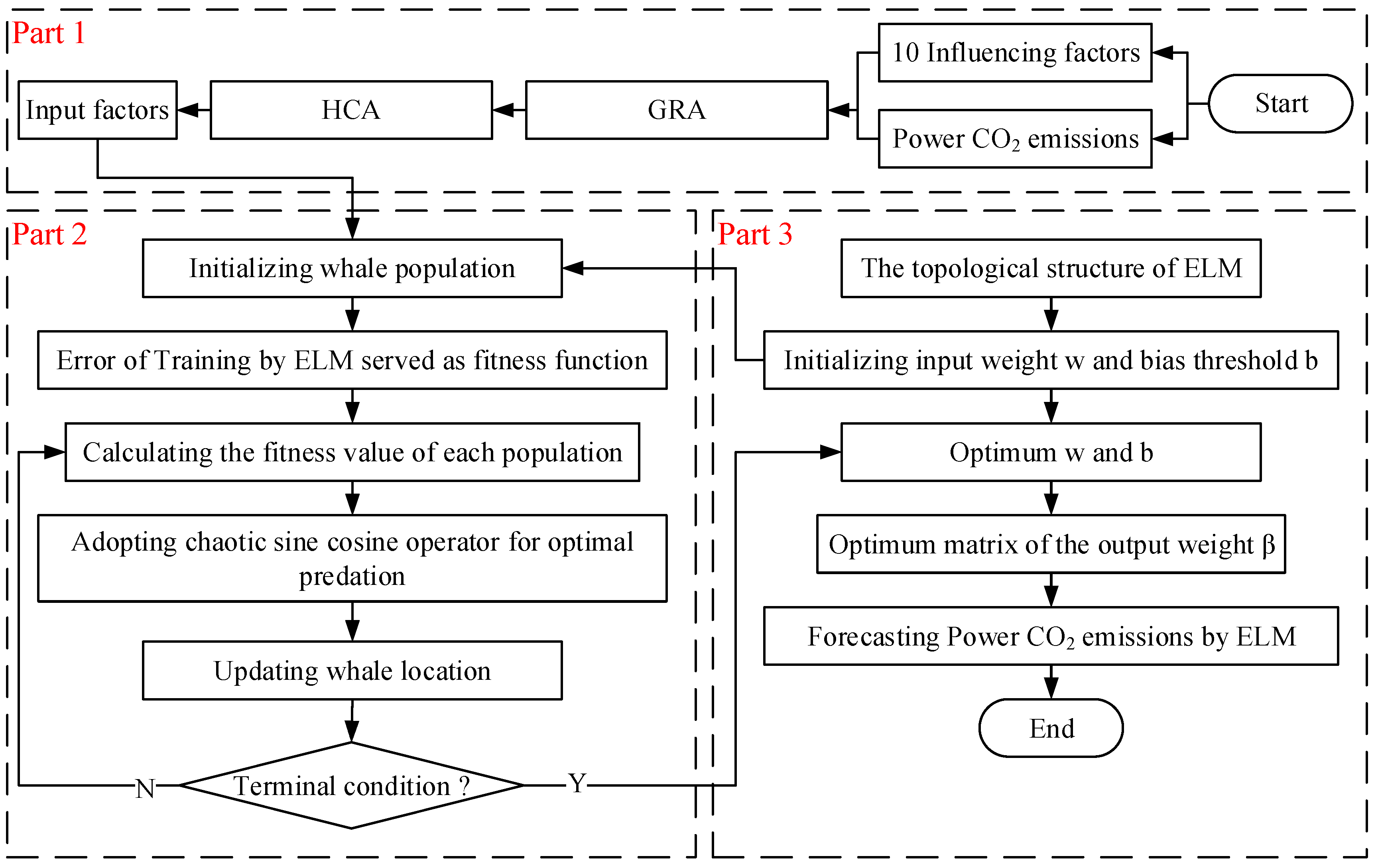
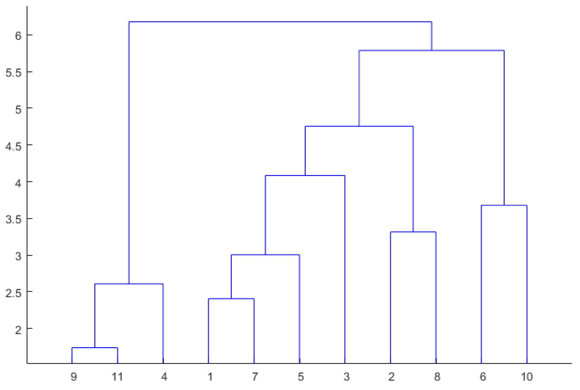
The remainder of this study is organized as follows. Firstly, the GRA is applied to select 11 influencing factors to form a perfect index system, highly correlated with power CO₂ emissions. Secondly, 5 key factors are exacted from 11 influencing factors as input values of the prediction model by HCA, aiming to reduce redundancy and keep information integrity. Thirdly, CSCWOA-ELM model is established to predict the powerCO₂ emissions, using 21 samples from 1992 to 2012 for training and 5 samples from 2013 to 2017 for testing. Finally, we put forward effective policy recommendations based on the above research.

2. Materials and Methods

In this section, the process of an extreme learning machine optimized by whale algorithm based on chaotic sine cosine operator (CSCWOA-ELM) establishment is described in detail.

2.1. Whale Optimization Algorithm Based on Chaotic Sine Cosine Operator (CSCWOA)

The whale optimization algorithm (WOA), a new group intelligent optimization algorithm, was proposed by Mirjalili et al. from Griffith University in 2016, simulating the hunting behavior of humpback whales [25]. The position of each humpback whale represents a feasible solution in the WOA algorithm, which has the advantages of simple operation and fewer adjustment parameters compared with other optimization algorithms. As the humpback whales navigate by the coordinates of optimal individual $X_{best}$ in the process of spiral predation, the convergence rate is accelerated, and the individuals of solution space aggregate rapidly, resulting in the accelerated decline of population diversity and the increased probability of the algorithm’s premature. In order to reduce the possibility of individuals gathering to local small areas, the sine cosine mechanism and chaos operator are introduced to control the motion regions of individuals, which improve the ability to jump out of local optimum [26]. In terms of the sine chaotic spiral predator movement (shown as Formula (1)), artificial whales use random individuals $X_{rand}$ as navigation coordinates to do sinusoidal logarithmic spiral motion, and search for food in a global context, which maintain the diversity of the population and avoid individual falling into local optimal solutions. Similarly, the cosine chaotic spiral predator movement (shown as Formula (2)) selects the optimal individual $X_{best}$ as the navigation coordinate, improving the speed of positioning during the optimization process.

$$X_{t+1}=X_t+r_1\cdot e^{b\cdot r_2}\cdot \sin \left(2\pi r_2\right)\cdot \left|r_3\cdot X_{rand}-X_t\right|$$

(1)

$$X_{t+1}=X_t+r_1\cdot e^{b\cdot r_2}\cdot \cos \left(2\pi r_2\right)\cdot \left|r_3\cdot X_{best}-X_t\right|$$

(2)

here, $r_3$ is the random number between [1,2], which controls the distance from the current individual $X_t$ to the random individuals $X_{rand}$ and the optimal individual $X_{best}$.Then, $r_1$ controls the range of regions for sinusoidal global search and cosine local development, of which the equation is:

$$r_1=a-a\cdot \frac{t}{T}$$

(3)

where $a$ is a constant; $t$ is the current number of iterations, and $T$ is the total number of iterations. As shown in the formula, $r_1$ adaptively decreases with the increase of the number of iterations, narrowing the optimization area. With the algorithm converging in the same optimal solution, convergence effect is guaranteed.

In addition, $b$ is the constant for shaping the spiral trajectory; $r_2$ is an optimization operator based on cubic chaotic map, which has better equilibrium ergodicity and convergence efficiency compared with the general chaotic operator sequence. The calculation process can be specified as follows:

$$r_2^{t+1}=\{\begin{array}{ll}rand\left[-1,1\right],& t=0\\ 4\cdot {\left(r_2^t\right)}^3-3\cdot r_2^t,& t\ge 1\end{array}$$

(4)

As shown in Formula (4), with the randomness and ergodicity of the chaotic map, the variation degree of the individuals is adaptively adjusted, enhancing the ability of the artificial whale to jump out of the local optimal solution in the sine cosine optimization.

As mentioned above, the sine chaotic global search helps the local development of cosine chaos to reduce the optimal blind spot, avoiding the loss of potential optimal solution. Conversely, the local development of cosine chaos compensates for the shortcoming of slow convergence in sine chaotic global search, which improves the efficiency of the algorithm. Comparing the progeny solutions generated by sine and cosine in chaotic prediction, the greedy mechanism is introduced to select the optimal solution [27]. To sum up, the sine cosine chaotic crossover optimization is adopted to avoid premature algorithm, aiming at improving the accuracy and calculation speed.

2.2. Extreme Learning Machine (ELM)

The multilayer perceptron (MLP) neural network trained by backpropagation algorithms is widely applied, which consists of input layer, hidden layer and output layer. ELM, composed of input layer, hidden layer and output layer, was proposed by Huang Guangbin to solve the single hidden layer feedforward neural network [28]. As the input weights and hidden layer thresholds are given randomly, the number of hidden layer nodes has a significant impact on the performance of the model. In terms of the single hidden layer feedforward neural network (SLFN), ELM utilizes the number of hidden network layers for network training, which greatly reduces the time and the computational complexity. Compared with other neural network algorithms, ELM has obvious advantages including faster learning speed, fewer input parameters, avoiding local extremum problems, and better generalization performance [29]. From the structure of the neural network, ELM is a simple SLFN (as shown in Figure 1). With fast learning speed and good generalization performance, ELM has attracted more attention from experts and scholars at home and abroad. However, the traditional ELM algorithm has the defect that the number of hidden layer nodes cannot be determined and the singularity problem is easy to occur [30].

2.3. Extreme Learning Machine Optimized by Whale Algorithm Based on Chaotic Sine Cosineoperator (CSCWOA-ELM)

As we know, the ELM output weight matrix is determined by the input weight matrix and the hidden layer threshold, which are randomly given during the training process. With the input weight matrix and hidden layer threshold invalid, the corresponding hidden layer node will be null [31]. As the number of hidden layer nodes directly affects the prediction accuracy of ELM, increasing the number of hidden layer nodes is the only way to improve the forecast accuracy, resulting in generalization problem at the same time.

In this paper, a new ELM optimized by whale algorithm based on chaotic sine cosine operator, is proposed to calculate the hidden layer weight, using the global optimization ability to optimize the connection weight $w_{ij}$ between the input layer and the hidden layer, and the neuron threshold $b_j$ in hidden layer. With the space occupied by hidden layer nodes reduced and the network structure simplified, the prediction model based on CSCWOA-ELM is established, which improves the regression prediction performance of neural networks with fewer hidden layer nodes. Furthermore, the sample data from 1992 to 2012 is selected as the training set, and the sample data from 2013 to 2017 as the test set. The prediction results indicate that the mean square error MSE = 0.00130 and the correlation coefficient R² = 0.99195, which means less error and high prediction accuracy. To sum up, CSCWOA-ELM is suitable for predicting the power CO₂ emissions in China. The specific implementation steps are shown as follows.

As illustrated in Figure 2, Based on literature research and characteristics of electric power industry, part 1 obtains 11 influencing factors of power CO₂ emissions by GRA. Furthermore, 5 key factors are extracted as the input variables of the prediction model by HCA. Part 2 is whale optimization algorithm based on chaotic sine cosine operator. In part 3, the ELM is adopted to forecast the power CO₂ emissions in China.

3. Data Analysis

In this section, the total carbon emissions of China’s power industry during 1992–2017 were calculated. Furthermore, key factors were selected by GRA and clustered by HCA. Eventually, 48 different development scenarios were set.

3.1. Data Sources and Usage

In this article, the initial data is from China Statistical Yearbook [32], International Energy Agency (IEA) and China Energy Statistics Yearbook [33,34]. In order to eliminate the price factors, the actual GDP and the living consumption level during 1992–2017 are converted into the constant price data based on 2005. Specifically, real GDP can be obtained by dividing the nominal GDP by the price index.

Up to now, there is no power CO₂ emissions data in China. Based on the carbon emission accounting method of energy balance sheet and the guidelines for China’s greenhouse gas (GHG) accounting methods for power generation enterprises, this paper calculates the power CO₂ emissions with the carbon emission coefficient of power generation fuels selected in IPCC 2006 [35]. Therefore, the calculation formula is as follows:

$$C={\displaystyle {\sum }_{i=1}^{n}F{C}_i}\times F{R}_i\times S\times E{F}_i$$

(5)

where $C$ is the amount of power CO₂ emissions; $i$ is the type of fuel for power generation; $F{C}_i$ is the consumption of the fuel $i$, and $F{R}_i$ is the standard coal conversion coefficient of the fuel $i$; $S$ is the low calorific value of the standard coal per kilogram, which is 29,307.6 kilojoules. $E{F}_i$ is the carbon emission coefficient of the fuel $i$. The calculation result of power CO₂ emissions from 1992 to 2017 is shown in Figure 3.

3.2. Grey Relational Analysis (GRA)

Throughout the study of predecessors, there are many influencing factors of power CO₂ emissions, which are not simply linearly related to the CO₂ emissions and present complex non-linear relationship. Namely, the impact of different factors on power CO₂ emissions is diverse. With all factors considered, it will have a negative impact on the prediction accuracy [36]. In terms of power generation, transmission and consumption, this paper selects11 factors by GRA, including population, living consumption level, GDP, thermal power conversion efficiency, urbanization rate, line loss rate, power structure, industrial structure, disposable income of residents, plant electricity consumption, and power generation structure. In particular, power structure refers to the proportion of thermal power installed capacity, and power generation structure is the proportion of thermal power production [37].

In this paper, power CO₂ emissions are selected as the parameter series. Furthermore, 11 influencing factors are selected as comparison series. The results of the correlation analysis are shown in

Table 1. Correlation analysis of 11 influencing factors.

Number	Influencing Factors	Correlation	Number	Influencing Factors	Correlation
1	GDP	0.934	7	disposable income of residents	0.814
2	living consumption level	0.917	8	urbanization rate	0.792
3	population	0.902	9	power generation structure	0.768
4	power structure	0.873	10	line loss rate	0.759
5	industrial structure	0.848	11	plant electricity consumption	0.752
6	thermal power conversion efficiency	0.822

.

As shown in Table 1, the 11 influencing factors have a strong correlation with the power CO₂ emissions, with the correlation degree all above 0.75. In addition, the impact of various influencing factors from high to low is GDP, living consumption level, population, power structure, industrial structure, thermal power conversion efficiency, disposable income of residents, urbanization rate, power generation structure, line loss rate, and plant electricity consumption.

3.3. Hierarchical Clustering Analysis (HCA)

As we all know, the GRA mainly studies the correlation between the influencing factors and the power CO₂ emissions, without exclusion and screening of the repeated influencing factors. In light of this, hierarchical clustering analysis, hereafter referred to as HCA, is adopted to eliminate the redundancy, with the influencing information retained.

Without knowing the number and structure of the categories, cluster analysis classifies a large number of observations into several classes, aiming at exposing a subset of observations in a data set. Particularly, HCA is most popular in many research fields [38]. According to the degree of similarity between the observed objects, the aggregation is carried out successively to achieve the purpose of clustering, that is, the distance between the individuals in the sample is replaced by the distance, and the samples with similar distances are placed in one class, which is repeated until the clustering is completed.

Based on the series of dimensionless processing in the GRA, the distance between each influencing factor is calculated, with the optimal class spacing selected by the composite coefficient R value. As shown in Figure 4, the clustering results of various influencing factors are obtained by MATLAB.

As shown in Figure 4, cluster analysis can classify different influencing factors into several categories, so as to find similarities between similarities and differences between different classes. Furthermore, analysis and reduction of redundancy between indicators can improve prediction accuracy. Based on the results of GRA and HCA, expert experience method is adopted to select 5 key factors in space family 7, including GDP, living consumption level, population, power structure, thermal power conversion efficiency.

3.4. Description of Scenarios

Obviously, various influencing factors have different trend in development, which means that setting a single forecasting scenario cannot cover the complex factors [39]. Therefore, this paper sets 48 different development scenarios based on different growth rates of the 5 influencing factors.

3.4.1. The Growth Rates of GDP

After a long-term sustained decline, China’s economic growth rate began to increase in 2016 and 2017. As the negative impact of financial crisis gradually decreases, the Chinese economy enters a stable period, referred as new economic normal. Based on the related research and economic development planning, the potential growth rate of GDP is set between 6–7% for 2018–2025, which are divided into high and medium categories (

Table 2. Values set for the growth rate of GDP from 2018 to 2025 (%).

Year	High Growth Rate	Medium Growth Rate
2018–2025	6.8	6.3

).

3.4.2. The Growth Rates of Living Consumption Level

According to the China Statistical Yearbook, the average annual growth rate of living consumption level from 2005 to 2017 was 12.79%. Simultaneously, the growth rate during 2014 to 2016 maintained around 9.5% [40]. With the economy revived and the living standard improved, the growth rate of living consumption level is expected to be steady and further promoted. Therefore, the growth rates are set to high, medium and low categories (

Table 3. Annual average growth rate of living consumption level from 2018 to 2025 (%).

Year	High Growth Rate	Medium Growth Rate	Low Growth Rate
2018–2025	15	12	9.5

).

3.4.3. The Growth Rates of Power Structure

In recent years, structural optimization policies, issued by the National Development and Reform Commission and the Energy Bureau, strictly limit the scale of thermal power, resulting in the proportion of installed thermal power capacity decreased by an average of 1.53%. The target of 13th Five-Year power structure adjustment target indicates that the installed capacity of non-fossil energy will increase to 39% of the total installed capacity, with the installed coal-fired capacity declined to 55% [41]. It is estimated that the investment and installed capacity of thermal power will be further controlled by government in the future. Therefore, the growth rates of power structure are set to high and medium categories (

Table 4. Power structure growth rates of China from 2018 to 2025 (%).

Year	High Growth Rate	Medium Growth Rate
2018–2025	−1.5	−1

).

3.4.4. The Growth Rate of Population

In the light of the China Statistical Yearbook, the natural growth rate of China’s population was around 0.5%from 2000 to 2017. The government has announced that the total population will be around 1.42 billion by 2020, with an average annual natural growth rate of 0.6% [42]. With the vigorous promotion of the comprehensive two-child policy, the population will increase in recent years. However, under the impact of the birth concept, the two-child policy will not make the population increase rapidly. Therefore, the population growth rates are set to medium and low categories (

Table 5. Values set for population growth rates of China from 2018 to 2025 (%).

Year	Medium Growth Rate	Low Growth Rate
2018–2025	0.8	0.6

).

3.4.5. The Growth Rates of Thermal Power Conversion Efficiency

With an average growth rate of 0.9%, the thermal power conversion efficiency has increased from 39.84% to 43.8% during 2005–2017. Specifically, the maximum growth rate was 1.9%, and the minimum was 0.02%. Based on the 13th five-year plan for power development, about 20 million kW backward coal-fired power units will be eliminated, aiming to upgrade coal-fired power [43]. Taking the technology and policies into consideration, the conversion efficiency of thermal power generation will maintain low or steady growth. In this paper, the growth rates of thermal power conversion efficiency are set to medium and low categories (

Table 6. Values set for conversion efficiency of thermal power in China from 2018 to 2025 (%).

Year	Medium Optimization Rate	Low Optimization Rate
2018–2025	1.5	0.5

).

As shown in

Table 7. Setting different development scenarios from 2018 to 2025.

Weakened Development Scenario						Base Development Scenario						Strengthened Development Scenario
SS	RG	EG	GS	PG	CG	SS	RG	EG	GS	PG	CG	SS	RG	EG	GS	PG	CG
WD1	Low	Medium	Medium	Low	Low	BD1	Medium	Medium	Medium	Low	Low	SD1	High	Medium	Medium	Low	Low
WD2	Low	Medium	Medium	Low	Medium	BD2	Medium	Medium	Medium	Low	Medium	SD2	High	Medium	Medium	Low	Medium
WD3	Low	Medium	Medium	Medium	Low	BD3	Medium	Medium	Medium	Medium	Low	SD3	High	Medium	Medium	Medium	Low
WD4	Low	Medium	Medium	Medium	Medium	BD4	Medium	Medium	Medium	Medium	Medium	SD4	High	Medium	Medium	Medium	Medium
WD5	Low	Medium	High	Low	Low	BD5	Medium	Medium	High	Low	Low	SD5	High	Medium	High	Low	Low
WD6	Low	Medium	High	Low	Medium	BD6	Medium	Medium	High	Low	Medium	SD6	High	Medium	High	Low	Medium
WD7	Low	Medium	High	Medium	Low	BD7	Medium	Medium	High	Medium	Low	SD7	High	Medium	High	Medium	Low
WD8	Low	Medium	High	Medium	Medium	BD8	Medium	Medium	High	Medium	Medium	SD8	High	Medium	High	Medium	Medium
WD9	Low	High	Medium	Low	Low	BD9	Medium	High	Medium	Low	Low	SD9	High	High	Medium	Low	Low
WD10	Low	High	Medium	Low	Medium	BD10	Medium	High	Medium	Low	Medium	SD10	High	High	Medium	Low	Medium
WD11	Low	High	Medium	Medium	Low	BD11	Medium	High	Medium	Medium	Low	SD11	High	High	Medium	Medium	Low
WD12	Low	High	Medium	Medium	Medium	BD12	Medium	High	Medium	Medium	Medium	SD12	High	High	Medium	Medium	Medium
WD13	Low	High	High	Low	Low	BD13	Medium	High	High	Low	Low	SD13	High	High	High	Low	Low
WD14	Low	High	High	Low	Medium	BD14	Medium	High	High	Low	Medium	SD14	High	High	High	Low	Medium
WD15	Low	High	High	Medium	Low	BD15	Medium	High	High	Medium	Low	SD15	High	High	High	Medium	Low
WD16	Low	High	High	Medium	Medium	BD16	Medium	High	High	Medium	Medium	SD16	High	High	High	Medium	Medium

Note: SS stands for scenario sequence; RG indicates the growth rates of living consumption level; EG is the growth rates of GDP; GS indicates the growth rates of power structure; PG is the growth rates of population; CG is the growth rates of thermal power conversion efficiency.

, based on the different rates of living consumption level, the development scenarios of power CO₂ emissions from 2018 to 2025 are set to 3 essential development scenarios, including the weakened development scenario (WD), the base development scenario (BD), and the strengthened development scenario (SD). In combination with the other four influencing factors, each essential development scenario is decomposed into 16 specific scenarios. As a consequence, this article totally sets up 48 specific scenarios.

4. Results and Discussions

In different essential development scenarios, the 5 key factors in16 specific scenarios are input into the CSCWOA-ELM model respectively. Ultimately, the predictions of powerCO₂ emissions can be obtained in different scenarios.

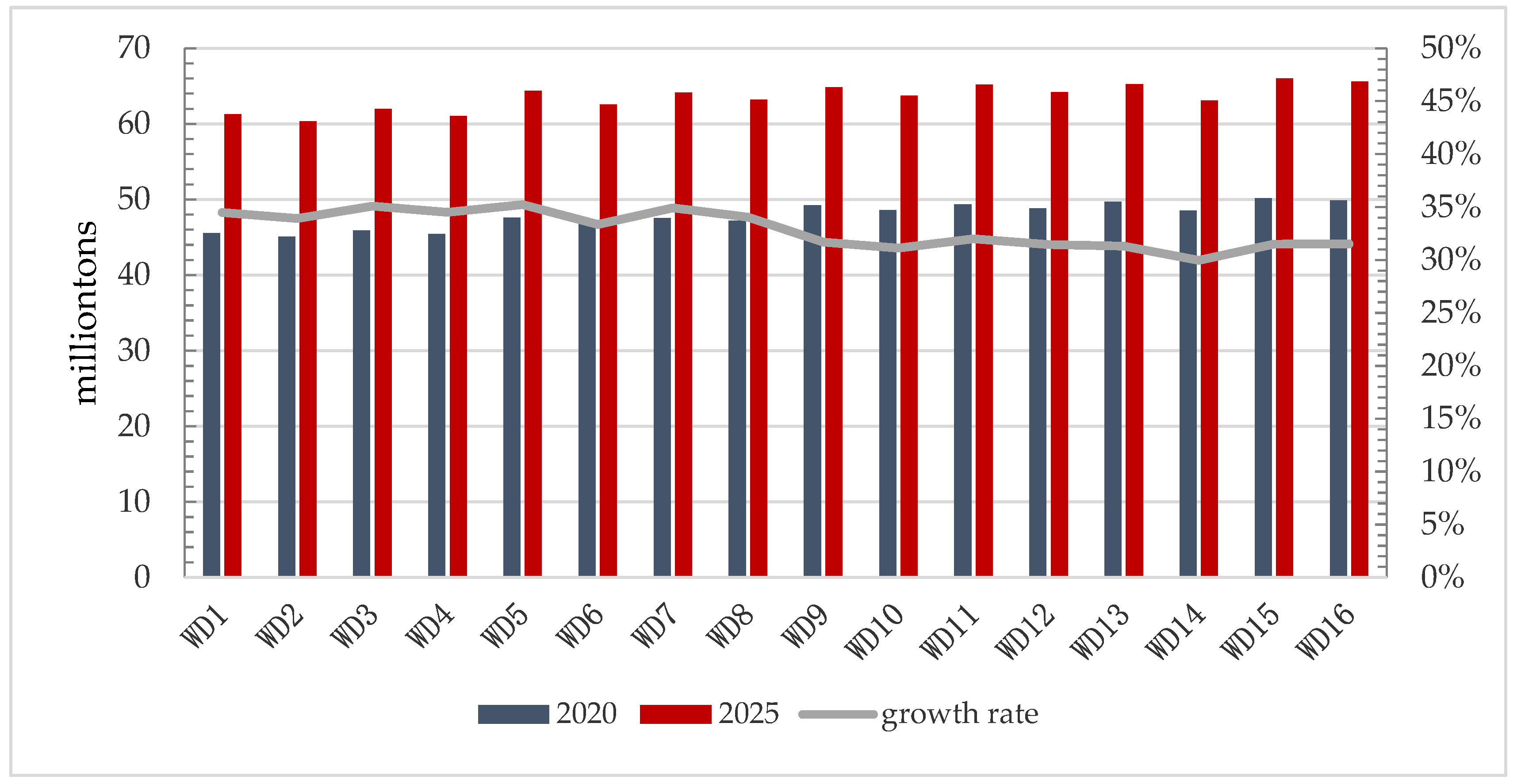
4.1. Predictions in the Weakened Development Scenario

The weakened development scenario includes 16 specific scenarios, with the low-speed growth rates of living consumption level. Meanwhile, the other four influencing factors select different growth rates. The results are shown in Figure 5.

As illustrated in Figure 5, the predictions of power CO₂ emissions will increase by 29.96–35.23% from 2020 to 2025 in the weakened development scenario. In detail, the growth rates will remain at 33.35–35.23% in the scenarios WD1–WD8, and at 29.96–31.99% in the scenarios WD9–WD16. In general, the power CO₂ emissions in the scenarios WD9–WD16 are more than those in the scenarios WD1–WD8. Particularly, the power CO₂ emissions in the scenario WD15 will reach a maximum, with the growth rates of GDP and power structure at high level, the population growth rate at medium level, and the growth rates of the living consumption level and the thermal power conversion efficiency at low level. Meanwhile, the power CO₂ emissions in the scenario WD2 will reach a minimum, with the growth rates of GDP, the growth rates of power structure and the growth rates of thermal power conversion efficiency at medium level, the growth rates of population and the living consumption level at low level.

Furthermore, the results indicate that the growth rates of thermal power conversion efficiency is negative correlation with the power the CO₂ emissions, while the others are positive. By comparing BD1 to BD9 (BD2 to BD10, BD3 to BD11, BD4 to BD12, BD5 to BD13, BD6 to BD14, BD7 to BD15, BD8 to BD16), the contribution rate of the GDP growth rate to the power CO₂ emissions is 1.24%. Similarly, the contribution rates of the power structure growth rate, the thermal power conversion efficiency growth rate, and the population growth rate are0.63%, 0.47%, and 0.35% respectively. Based on the above, the contribution rates of the4 influencing factors from high to low are the growth rates of GDP, the growth rates of power structure, the growth rates of thermal power conversion efficiency, and the growth rates of population. As the growth rate of GDP increase by 1%, the power CO₂ emissions will rise 1.24%. Similarly, the growth rate of power structure, the growth rate of thermal power conversion efficiency, and the growth rate of population increase by 1%, with the power CO₂ emissions rising0.63%, 0.47%, and 0.35% in turn.

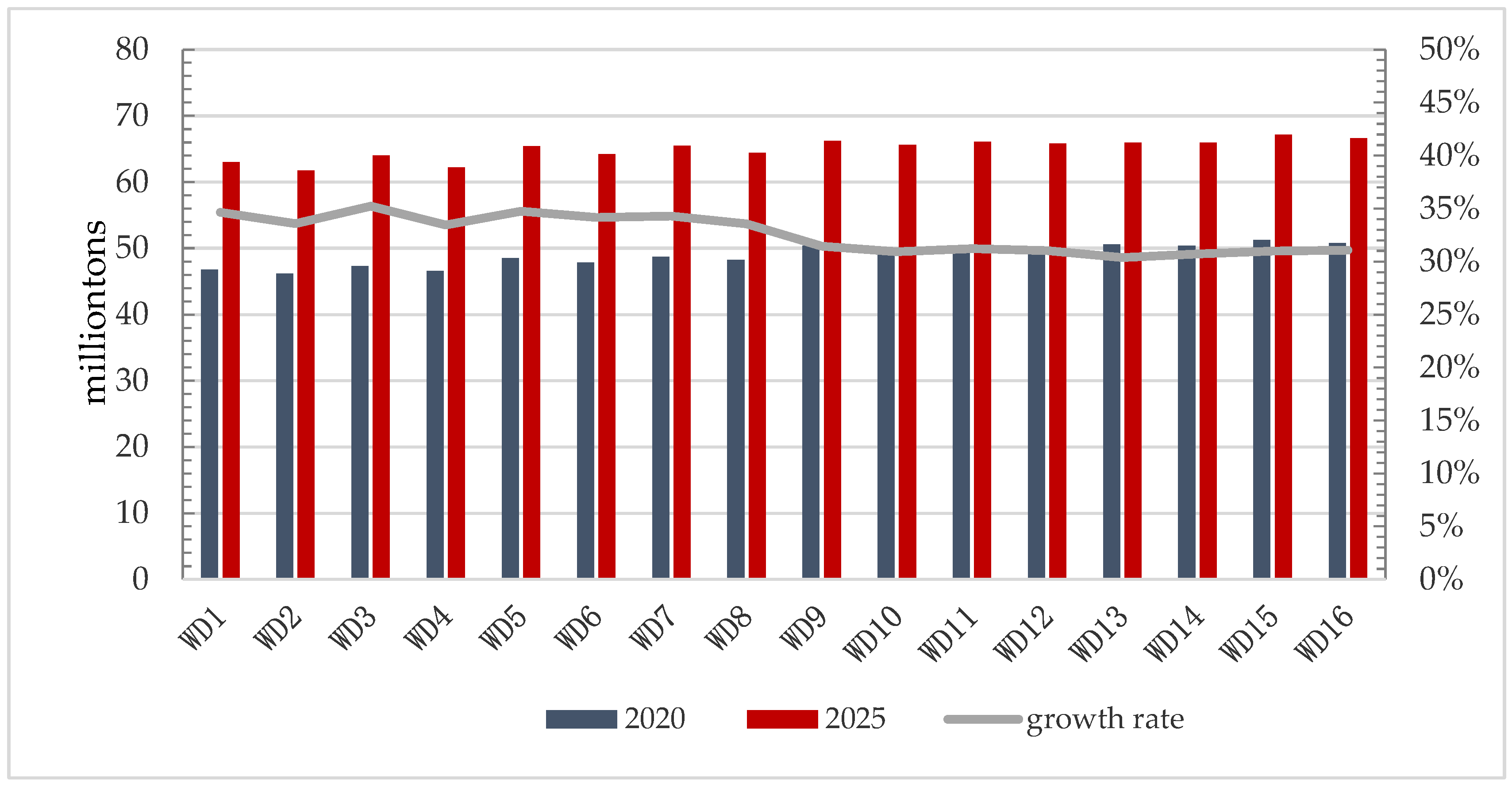
4.2. Predictions in the Based Development Scenarios

The based development scenario includes 16 specific scenarios, with the medium growth rates of living consumption level. As the other four influencing factors select different growth rates, the predictions of power CO₂ emissions are shown in Figure 6.

According to Figure 6, compared with 2020, the predictions of power CO₂ emissions in 2025 will increase by 30.38–35.22% in the based development scenario. In detail, the growth rates will remain at 33.46–35.22% in the scenarios WD1–WD8, and at 30.38–31.44% in the scenarios WD9–WD16. Furthermore, the power CO₂ emissions in the scenarios WD9-WD16 are higher than those in the scenarios WD1–WD8. Obviously, the power CO₂ emissions in the scenario WD15 will reach a maximum, with the growth rates of GDP and power structure at high level, the growth rates of living consumption level and population at medium level, and the growth rates of thermal power conversion efficiency at low level. In addition, the power CO₂ emissions in the scenario WD2 will reach a minimum, with the growth rates of population at low level, and the others at medium level.

By comparing BD1 to BD9 (BD2 to BD10, BD3 to BD11, BD4 to BD12, BD5 to BD13, BD6 to BD14, BD7 to BD15, BD8 to BD16), the contribution rate of the GDP growth rate to the power CO₂ emissions is 1.33%. Similarly, the contribution rates of the power structure growth rate, the thermal power conversion efficiency growth rate, and the population growth rate are 0.61%, 0.46%, and 0.37% respectively. Therefore, the contribution rates of the 4 influencing factors are ordered in turn: the growth rate of GDP, the growth rate of power structure, the growth rate of thermal power conversion efficiency, and the growth rate of population. As the growth rate of GDP increases by 1%, the power CO₂ emissions will rise 1.33%. Similarly, the growth rates of power structure, thermal power conversion efficiency, and population increase by 1%, leading to the power CO₂ emissions rising 0.61%, 0.46%, and 0.37% respectively.

4.3. Predictions in the Strengthened Development Scenarios

The strengthened development scenario includes 16 specific scenarios, with the living consumption levels all maintaining high growth rates. Meanwhile, the other 4 influencing factors select different growth rates. The predictions of power CO₂ emissions in 2020 and 2025 are shown in Figure 7.

As shown in Figure 7, the predictions of the power CO₂ emissions will increase by 29.68–35.16% from 2020 to 2025 in the strengthened development scenario. Specifically, the growth rates will remain at 33.44–35.16% in the scenarios WD1–WD8, and at 29.68–32.06% in the scenarios WD9–WD16. Generally, the power CO₂ emissions in the scenarios WD9–WD16 are higher than those in the scenarios WD1–WD8. In particular, the power CO₂ emissions in the scenario WD15 will reach a maximum, with the growth rates of GDP, living consumption level, and power structure at high level, the growth rates of population at medium level, and the growth rates of thermal power conversion efficiency at low level. Simultaneously, the power CO₂ emissions in the scenario WD2 will reach a minimum, with the growth rates of living consumption level at high level, the population growth rate at low level, and the others at medium level.

By comparing BD1 to BD9 (BD2 to BD10, BD3 to BD11, BD4 to BD12, BD5 to BD13, BD6 to BD14, BD7 to BD15, BD8 to BD16), the contribution rate of the GDP growth rate to the power CO₂ emissions is 1.28%. Similarly, the contribution rates of the power structure growth rate, the thermal power conversion efficiency growth rate, and the population growth rate are 0.61%, 0.5%, and 0.38% respectively. Based on the above, the contribution rates of the 4 influencing factors ordered from high to low are the growth rate of GDP, the growth rate of power structure, the growth rate of thermal power conversion efficiency, and the growth rate of population. As the growth rate of GDP increases by 1%, the power CO₂ emissions will rise 1.28%. Similarly, the growth rates of power structure, thermal power conversion efficiency, and population increase by 1%, resulting in the power CO₂ emissions rising 0.61%, 0.5%, and 0.38% respectively. In addition, through the comparison of WD1, BD1, and SD1 (WD2, BD2, and SD2; WD3, BD3, and SD3; ...; WD16, BD16, and SD16), the contribution rate of the living consumption level growth rate is 0.76%. That is, when the growth rate of living consumption level increases by 1%, the power CO₂ emissions will rise 0.76%.

4.4. Comparisons of the Three Essential Development Scenarios

As shown in the comparison results, the power CO₂ emissions in the corresponding specific scenarios from the three essential scenarios, such as WD1, BD1 and SD1 (WD2, BD2 and SD2, WD3, BD3, and SD3; ...; WD16, BD16, and SD16), increase in turn. Furthermore, the growth rates of the power CO₂ emissions show a significant decline in general, fluctuating between 29.68–35.23%. Meanwhile, it is found that GDP, power structure, and the living consumption level are the main influencing factors of the power CO₂ emissions, with the contribution rates all above 0.6%. Nevertheless, the impacts of the thermal power conversion efficiency and population are small, with the contribution rates less than 0.5%. As consequence, the contribution rates of each influencing factor in the three essential scenarios are shown in

Table 8. Comparison results of the three essential development scenarios from 2018 to 2025.

Contrastive Terms	WD	BD	SD
Predictions of power CO2 emissions	lower	average	higher
Moving trend of the power CO2 emissions growth rate from 2020 to 2025	WD1–WD8: 33.35–35.23%; WD8–WD9: 29.96–31.99%	BD1–BD8: 33.46–35.22%; BD8–BD9: 30.38–31.44%	SD1–SD8: 33.44–35.16%; SD8–SD9: 29.68–32.06%
The contribution rates of GDP	1.24%	1.33%	1.28%
The contribution rates of living consumption level	0.76%	0.76%	0.76%
The contribution rates of the power structure	0.63%	0.61%	0.61%
The contribution rates of the thermal power conversion efficiency	0.47%	0.46%	0.51%
The contribution rates of population	0.35%	0.37%	0.38%

.

5. Conclusions

In this study, based on the correlation of influencing factors, 5 key factors are selected from 11 influencing factors through HCA. Furthermore, the prediction model of CSCWOA-ELM is established to forecast the power CO₂ emissions in 48 specific development scenarios, with the contribution rates of 5 influencing factors calculated. Through the comparison within the three essential development scenarios, it is regarded as evident to conclude that: (1) With an average contribution rate of 1.28%, GDP is the biggest influencing factor of the power CO₂ emissions. (2) With an average contribution rate of 0.62%, the power structure is also a significant influencing factor. Through the comparison among the three essential development scenarios, we can draw the conclusion that: (3) the average contribution rate of the living consumption level is 0.76%, which is higher than that of the power structure. To sum up, GDP, the power structure, and the living consumption level are the most important influential factors of the power CO₂ emissions in China.

As we know, the power output in China generates a large number of CO₂, posing a serious threat to the reduction of CO₂ emissions. Based on the above, some recommendations for the reduction of the power CO₂ emissions in China are proposed as follows: (1) As industry plays a significant role in China’s economy, the industrial power consumption accounts for around 71.6% of the total, and the unit power consumption is 23.45 kWh/million, which was 15.95 times than that of the service. Therefore, it is recommended that High-tech industries and service industry should be promoted to achieve the economic growth without considerable CO₂ emissions. (2) The thermal power production, accounting for around 73.7% of power output, is main source of CO₂ emissions, resulting in serious air pollution. Hence, improving the proportion of clean power generation is an effective measure to reduce power CO₂ emissions, based on the implementation of clean energy policies. Furthermore, new technologies and equipment should be applied to increase the conversion efficiency of thermal power, which is conducive to reducing the consumption of coal and petroleum. (3) With regard to the power waste, more attention should be taken to the awareness of energy conservation. With the living standards improving gradually, the degree of household electrification continues to increase, driving the power consumption and CO₂ emissions. In order to solve the above problem, the government should also strengthen propaganda to cultivate the conservation awareness, and the focus of emission reduction should be concentrated on the optimization of the power structure. Finally, these recommendations can be regarded as a reference for China’s 14th Five-Year development to cut down CO₂ emissions.

References

1. Wang, Y.; Cheng, Y.; Yang, G.Y.; Dong, Y. Provincial Decomposition of China’s Carbon Emissions Rights Under the Constraint of 2020 and 2030 Carbon Intensity Targets. China Environ. Sci. 2018, 38, 3180–3188. [Google Scholar]
2. Li, Q.Q.; Su, Y.; Shang, L.; Wei, W.; Wang, M.H. Comparison Analysis of China’s Emissions Accounting by Typical International Carbon Databases. Clim. Chang. Res. 2018, 14, 275–280. [Google Scholar]
3. Global Carbon Atlas. Available online: http://www.globalcarbonatlas.org/cn/CO2-emissions (accessed on 3 April 2018).
4. Li, Q. Carbon Emissions Analysis and Forecast of High Energy-Consuming Industries in China; Tianjin University: Tianjin, China, 2016. [Google Scholar]
5. Ma, X.J.; Wang, Y.; Wang, C. Low-carbon Development of China’s Thermal Power Industry Based on an International Comparison: Review, Analysis and Forecast. Renew. Sustain. Energy Rev. 2017, 80, 942–970. [Google Scholar] [CrossRef]
6. Dong, K.Y.; Sun, R.J.; Dong, X.C. CO2 Emissions, Natural Gas and Renewables, Economic Growth: Assessing the Evidence from China. Environ. Sci. 2018, 640, 293–302. [Google Scholar] [CrossRef] [PubMed]
7. People.cn. What Commitments Has China Made to Respond to Global Climate Change? Available online: http://world.people.com.cn/n/2015/1201/c1002-27877413.html (accessed on 8 May 2018).
8. China Carbon Trading Network. Path Optimization for China’s 2030 Carbon Emission Peak Target. Available online: http://www.tanjiaoyi.com/article-23830-1.html (accessed on 10 June 2018).
9. Li, L.; Lei, Y.L.; Wu, S.M.; He, C.Y.; Chen, J.B.; Yan, D. Impacts of City Size Change and Industrial Structure Change on CO2 Emissions in Chinese Cities. Clean. Prod. 2018, 195, 831–838. [Google Scholar] [CrossRef]
10. National Development and Reform Commission. Outline of the Thirteenth Five-Year Plan for National Economic and Social Development of the People’s Republic of China. Available online: http://www.ndrc.gov.cn/zcfb/zcfbghwb/201603/P020160318573830195512.pdf (accessed on 11 June 2018).
11. Zhao, X.L.; Ma, Q.; Yang, R. Factors Influencing CO2 Emissions in China’s Power Industry: Co-integration Analysis. Energy Policy 2013, 57, 89–98. [Google Scholar] [CrossRef]
12. Klein, D.E. CO2 Emissions Trends for the US and Electric Power Sector. Electr. J. 2016, 29, 33–47. [Google Scholar]
13. Chai, Q.M.; Fu, S.; Zheng, X.Q.; Zhao, X.C.; Xu, Q.H. Carbon Emission Cap Control Target and Policy Study of Selected Sectors and Industries in China. China Popul. 2017, 27, 1–7. [Google Scholar]
14. Ma, D.; Shan, B.G.; Zhu, F.A. Vision of Medium-and Long-Term Energy Demand Based on CO2 Emission Peak Target. Electr. Power 2017, 50, 180–185. [Google Scholar]
15. Huo, M.L.; Han, X.Y.; Shan, B.G. Empirical Analysis of Factors Affecting Carbon Emission Intensity in China’s Power Industry. China Power 2013, 4, 122–126. [Google Scholar]
16. Hou, J.C.; Tan, Z.F. Decomposition of CO2 Emission Changes in Electric Power Production. China Power 2011, 44, 39–42. [Google Scholar]
17. Wang, C.K.; Xie, H.Z. Dynamic Characteristics and InfluencingFactors of China’s Power Carbon Emissions. China’s Popul. Resour. Environ. 2015, 25, 21–27. [Google Scholar]
18. Zhang, M. Research on Influence Factors of Carbon Emission from Power Industry in Jing-Jin-Ji Region Based on LMDI; North China Electric Power University: Beijing, China, 2017. [Google Scholar]
19. Wang, Y.H.; Luo, J. Research on Potential and Mechanism of Emission Reduction in Power Industry: Taking Sichuan as an Example. Jiangxi Soc. Sci. 2013, 5, 87–92. [Google Scholar]
20. Xu, J. Baoding Electric Power Industry Carbon Emission Measurement and Forecast. J. Hebei Univ. 2014, 34, 122–128. [Google Scholar]
21. Liu, L.W.; Zong, H.; Zhao, E.D.; Chen, C.X.; Wang, J.Z. Can China Realize Its Carbon Emission Reduction Goal in 2020: From the Perspective of Thermal Power Development. Appl. Energy 2014, 124, 199–212. [Google Scholar] [CrossRef]
22. Zhang, Q.Q.; Zhu, C.Z. Study on the Potential of CO2 Reduction in Industry in Anhui Province. J. Anhui Univ. Technol. 2014, 31, 433–437. [Google Scholar]
23. Wang, X.P.; Wang, Y.Y. System Dynamics Based Prediction of Carbon Emission in Power Industry. Shaanxi Electr. Power 2016, 44, 29–32. [Google Scholar]
24. Wang, Y.; Bi, Y.; Wang, E.D. Scene prediction of carbon emission peak and emission reduction potential estimation in Chinese industry. China’s Popul. Resour. Environ. 2017, 27, 131–140. [Google Scholar]
25. Mirjalili, S.; Lewis, A. The Whale Optimization Algorithm. Adv. Eng. Softw. 2016, 95, 51–67. [Google Scholar] [CrossRef]
26. Mirjalili, S. Sca: ASine Cosine Algorithm for Solving Optimization Problems. Knowl. Based Syst. 2016, 96, 120–133. [Google Scholar] [CrossRef]
27. Wang, X.; Li, Z.Y.; Xu, G.Y.; Wang, Y. Artificial Bee Colony Algorithm Based on Chaos Local Search Operator. J. Comput. Appl. 2012, 32, 1033–1036. [Google Scholar] [CrossRef]
28. Sun, X.Y.; Hu, J.T.; Wang, Z.; Zhang, J.L. Online Prediction Method for Generation and Consumption of Blast Furnace Gas Based on Adaptive Forgetting Factor Extreme Learning Machine. Comput. Meas. Control 2017, 25, 235–238. [Google Scholar]
29. Fan, J.; Wang, X.; Xu, H. Prediction Method of Tectonic Coal Thickness Based on Particle Swarm Optimized Hybrid Kernel Extreme Learning Machine. J. Comput. Appl. 2018, 38, 1820–1825. [Google Scholar]
30. Chen, X.Q.; Lu, H.J.; Zheng, W.B.; Yan, K. Optimization of Extreme Learning Machine Parameters by Adaptive Chaotic Particle Swarm Optimization Algorithm. J. Comput. Appl. 2016, 36, 3123–3126. [Google Scholar]
31. Xu, C.C.; Xu, X.Y.; Yan, G.W.; Han, X.X. NOX Emission Prediction Algorithm of Power Station Boiler Based on Improved Distributed Extreme Learning Machine. J. Taiyuan Univ. Technol. 2017, 48, 946–952. [Google Scholar]
32. National Bureau of Statistics. China Statistical Yearbook. Available online: http://www.stats.gov.cn/tjsj/ndsj/ (accessed on 15 August 2018).
33. International Energy Agency. Emissions Factors Methodology. 2017. Available online: https://webstore.iea.org/emissions-factors (accessed on 4 August 2018).
34. National Bureau of Statistics. China Energy Statistical Yearbook. Available online: http://www.stats.gov.cn/tjsj./tjcbw/201806/t20180612_1604117.html (accessed on 20 August 2018).
35. National Development and Reform Commission. The Guidelines and Reporting Guidelines (Trial) for the Second Batch of Enterprises’ GHG Emissions in 4 Industries. Available online: http://qhs.ndrc.gov.cn/zcfg/201502/t20150209_663603.html (accessed on 25 April 2018).
36. Liu, H.; Wu, J.; Geng, G.H. Research on High-interest Data Mining Algorithm Based on Grey Relational Analysis. Comput. Eng. Des. 2008, 29, 4242–4244. [Google Scholar]
37. Li, Z.Z. Study on the Influence Factors of Consumption Level of Residents in Henan Based on Grey Correlation Analysis. Value Eng. 2018, 10, 176–177. [Google Scholar]
38. Ratto, G.; Berri, G.J.; Maronna, R. On the Application of Hierarchical Cluster Analysis for Synthesizing Low-Level Wind Fields Obtained with aMesoscale Boundary Layer Model. Meteorol. Appl. 2014, 21, 708–716. [Google Scholar] [CrossRef]
39. Li, J.Y.; Shi, J.F.; Li, J.C. Exploring Reduction Potential of Carbon Intensity Based on Back Propagation Neural Network and Scenario Analysis: A Case of Beijing. Energies 2016, 9, 615. [Google Scholar] [CrossRef]
40. Dong, J.P.; Chen, G.D.; Yang, Z.Y. Research on theThreshold Effect of Household Consumption Level on Carbon Emission in Life. Arid Zone Resour. Environ. 2017, 31, 38–43. [Google Scholar]
41. Liu, T.; Bai, H.T.; Xu, H. Decomposition of Carbon Emission Drivers for Electricity Consumption in Typical Regions of China. Environ. Pollut. Prev. 2017, 39, 1278–1283. [Google Scholar]
42. Wu, C. Low-Carbon Policy and Action in the Chinese Mainland: An Overview of Current Development. Chin. Stud. 2014, 3, 157–164. [Google Scholar]
43. Yang, L.; Lin, B. Carbon Dioxide-emission in China’s Power Industry: Evidence and policy implications. Renew. Sustain. Energy Rev. 2016, 60, 258–267. [Google Scholar] [CrossRef]
Figure 1. The structure of Extreme Learning Machine (ELM) model.
Energies 11 02709 g001
Figure 2. Application process of the extreme learning machine optimized by whale algorithm based on chaotic sine cosine operator (CSCWOA-ELM) model.
Energies 11 02709 g002
Figure 3. The power CO2 emissions of China from 1992 to 2017.
Energies 11 02709 g003
Figure 4. Cluster diagram of various influencing factors.
Energies 11 02709 g004
Figure 5. The predictions of power CO2 emissions for the weakened development scenario in 2020 and 2025.
Energies 11 02709 g005
Figure 6. The predictions of power CO2 emissions for the based development scenario in 2020 and 2025.
Energies 11 02709 g006
Figure 7. The predictions of power CO2 emissions for the strengthened development scenario in 2020 and 2025.
Energies 11 02709 g007