A Semi-Analytical Method for Simulating Two-Phase Flow Performance of Horizontal Volatile Oil Wells in Fractured Carbonate Reservoirs

Abstract

Two-phase flow behavior in fractured carbonate reservoirs was investigated due to the importance for geothermal and petroleum resource recovery, such as in this study the phase change of volatile oil. This paper presents a semi-analytical method for accurately modeling two-phase flow behavior and quickly predicting the production performance. The fractured carbonate reservoir was modeled with a dual-porosity model, and the phase change and two-phase flow were modeled using the black oil model. The production of the oil phase was obtained through linearizing and solving the mathematical model. The gas phase production was forecast using the producing gas-oil ratio (GOR), calculated using flowing material balance equations. By comparing the semi-analytical solution to the solution of the commercial numerical simulator and applying it to a field case, the accuracy and practicability of the proposed semi-analytical method could be validated. Based on the semi-analytical model, the influences of several critical parameters on production performance were also analyzed. The proposed model was shown to be efficient in evaluating two-phase production performance of horizontal volatile oil wells. Furthermore, the new technique is able to serve as a useful tool for analyzing two-phase production data and making forecasts for volatile oil wells in fractured carbonate reservoirs.

1. Introduction

With the degree of deepening exploration and adoption of advanced technology, the exploitation of fractured carbonate volatile oil reservoirs has been attracting considerable attention in recent years [1,2,3,4]. Meanwhile, the application of horizontal wells not only increases the drainage area but also enhances production of a single well. Analyzing the performance of horizontal wells has become more and more popular among engineers [5,6,7,8,9,10,11,12]. The two-phase flow of oil and gas is quite common and hard to simulate in volatile oil reservoirs. The fractured carbonate volatile oil reservoir is rather complicated because of its complex reservoir architecture and fluid properties. A big challenge is that the phase change, pressure dependent properties, and two-phase flow behavior and stress-dependent fracture permeability should be all considered when developing the mathematical model of fractured carbonated volatile oil reservoirs. The current method to establish horizontal volatile oil wells is mainly depletion. It is crucial to predict the production and analyze two-phase production data from this kind of well, and much research has been done on theoretical models of horizontal wells in fractured carbonate reservoirs [13,14,15,16,17]. However, most of them are only applicable to the single-phase flow problem. Moreover, little to no research has been performed on the production performance of horizontal volatile oil wells in fractured carbonate reservoirs.

Recently, researchers became interested in the study of two-phase flow modeling of horizontal wells in volatile oil reservoirs [1,2,3,4,7]. Empirical, semi-analytical and numerical methods have been widely used for two-phase production data analysis. Empirical methods [18,19,20,21,22,23,24] are commonly applied in the actual oil field to conduct history matching and make forecasts for production wells because they are easy to use. However, these methods are only suitable for specific conditions and generally inappropriate for the two-phase flow problem. Conventional methods have used numerical simulations [25,26,27,28,29] for modeling two-phase flow behavior of horizontal volatile oil wells, but gridding and simulating are time-consuming.

Modeling the two phase flow characteristics is a key part in the numerical simulation of petroleum development. There are mainly two semi-analytical methods to capture the two-phase flow behavior. The first method is based on Perrine’s [30] and Martin’s [31] assumption, in which two-phase flow could be reduced to single-phase flow by defining a two-phase pseudo-pressure. According to Perrine’s approach [30], the relationship between saturation and pressure is constant and should be known in advance. In addition, laboratory PVT tests are needed to evaluation this relationship. Fetkovich [32], Raghavan et al. [33,34,35,36], as well as Ng and Aguilera [37] proposed a procedure to obtain the relationship from producing the gas–oil ratio. Actually, the flow equations are still mathematically nonlinear; this is because the relative permeability is a function of saturation. Also, oil density and the formation volume factor are functions of reservoir pressure. However, both the saturation and pressure in the reservoir are unknown parameters. The second method is by using the similarity method [38,39,40,41,42,43,44,45], which uses the Boltzmann transformation to turn the partial governing equations (PDEs) into ordinary differential equations (ODEs). O’Sullivan [38] firstly introduced the similarity method in the study of the two-phase flow problem. Bøe et al. [39] and Kissling et al. [40] extended O’Sullivan work by using the Boltzmann transformation to turn PDEs into ODEs. Ayala and Kouassi [41] and Zhang and Ayala [42] expanded the Bøe’s approach to cover the transient linear flow condition. The advantages of using the similarity method lie in two aspects, the first is that the relationship between saturation and pressure does not need to be known in advance, and the second is that the solutions of the equations could be solved accurately if the PDEs could be transformed into ODEs [43,44,45]. However, the similarity method is only suitable for transient linear flow regime, rather than dual porosity models. Recently, Clarkson and Qanbari [46,47] proposed an approximate semi-analytical method to analyze two-phase production data for fractured tight reservoirs, in which the producing gas-oil ratio (GOR) is used to forecast gas production. Generally, current research on the semi-analytical methods mostly focuses on the fractured tight reservoirs. Moreover, relatively less research on horizontal volatile wells in fractured carbonate reservoirs has been found in public literature. Therefore, proposing an effective semi-analytical method to capture the two-phase flow behavior of horizontal volatile oil wells in fractured carbonate reservoirs is of significant importance.

In this study, a novel semi-analytical method is presented to simulate the two-phase flow behavior of horizontal volatile oil wells in fractured carbonate reservoirs. A dual-porosity, black oil model considering phase change and two-phase flow is applied to model the fractured carbonate reservoirs. The model takes into account the complexities of phase change, pressure dependent PVT properties, two-phase flow behavior, and permeability stress sensitivity characteristics in the reservoir. The governing equations are linearized using a successive iteration method. With Laplace transform and separation of variable, one can obtain the analytical solution of the mathematical model. After getting the production of the oil phase from the previous time step, the average pressure and saturation within the investigated area are calculated with the flowing material balance equation. Calculations are then repeated for this time step to update the model parameters and the producing GOR with the Newton-Raphson scheme, followed by a novel proposed procedure for history matching of field production data and production forecasts. The semi-analytical method is benchmarked against the commercial simulator Eclipse. Furthermore, the effects of some critical parameters on production performance are also analyzed with the proposed model. Finally, a field example from the eastern Pre-Caspian basin is used to demonstrate the practicability of the method.

2. Methodology

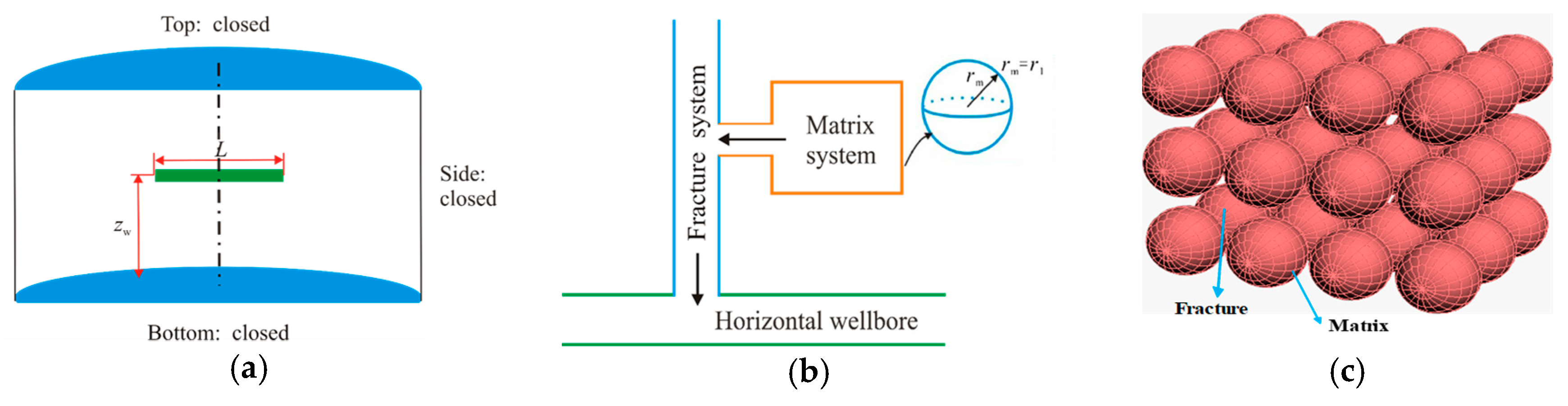
2.1. Model Assumption

As shown in Figure 1, the fractured carbonate reservoir is modeled with a classical dual-porosity model [15], which is composed of fracture and matrix systems. A radial cylindrical dual-porosity medium reservoir is considered in which a single horizontal well is located at the center, which completely penetrates the formation. The dual-porosity model assumes the fracture system is the flow pathway directly connected to the wellbore, fluids in the fracture system first flow into the horizontal wellbore, followed by the matrix-fracture inter-porosity flow. The volatile oil consists of two components, which are dead oil and dry gas. During depletion development, the process of gas dissolving and separating from the oil phase is considered, but oil dissolved in the gas phase is neglected. Some simplifying physical model assumptions for the derivation of the governing equation are listed as: The horizontal well is produced with constant bottom-hole pressure in the fractured carbonate reservoir, and the external boundaries of the top, bottom, and side are all assumed to be closed. The spherical matrix blocks are considered in the model to describe the matrix-fracture inter-porosity flow [48]. Fluid flow follows the law of Darcy seepage, and stress-dependent fracture permeability is considered. Also, capillary and gravity forces are neglected to simplify the model.

2.2. Mathematical Model

In this paper, a semi-analytical method is proposed to simulate two-phase flow behavior and make forecasts of horizontal volatile oil wells in fractured carbonate reservoirs. The forecasted producing GOR is used to reduce the equations of the two-phase flow model, so only the flow equations of the oil phase are used to develop the mathematical model. The production rate of the oil phase is obtained with the solution of the mathematical model, and the production rate of the gas phase is calculated by using the producing GOR. In the following, a simplified black oil model is used to analyze two-phase performance from this kind of well. The process of gas dissolving and separating from the oil phase is considered, while oil dissolved in the gas phase is neglected. After some reasonable assumptions and simplification, the mathematical model was established in a radial cylindrical system.

The governing differential equation of the fracture system is expressed as follows [10]:

$$\frac{1}{r}\frac{\partial }{\partial r}\left[r\left(\frac{k_{\mathrm{fro}}}{{\mu }_{\mathrm{o}}{B}_{\mathrm{o}}}\right)\frac{\partial p_{\mathrm{f}}}{\partial r}\right]+\frac{k_{\mathrm{fv}}}{k_{\mathrm{fh}}}\frac{\partial }{\partial z}\left(\frac{k_{\mathrm{fro}}}{{\mu }_{\mathrm{o}}{B}_{\mathrm{o}}}\frac{\partial p_{\mathrm{f}}}{\partial z}\right)+\frac{q_{\mathrm{oMf}}}{k_{\mathrm{fh}}}=\frac{{\varphi }_{\mathrm{f}}}{{\alpha }_{\mathrm{c}}{k}_{\mathrm{fh}}}\frac{\partial }{\partial t}\left(\frac{S_{\mathrm{o}}}{B_{\mathrm{o}}}\right)$$

(1)

where r is the radial distance in reservoir formation, m; z is the perpendicular distance from bottom, m; μ_o represents the oil viscosity, mPa·s; B_o represents the oil formation volume factor, fraction; p_f represents the fracture-system pressure, MPa; ϕ_f represents the fracture-system porosity, fraction; k_fh represents the formation permeability of fracture-system, mD; k_fv is the perpendicular permeability of the fracture-system, mD; k_fro represents the oil relative permeability of the fracture-system, fraction; q_oMf represents the inter-porosity flow rate per unit matrix volume; α_c represents the conversion factor, fraction; S_o represents the oil saturation, fraction; t is the time, h.

The inter-porosity flow rate, q_oMf can be written as [48]

$$q_{\mathrm{oMf}}=-\frac{3}{r_1}\frac{k_{\mathrm{M}}{k}_{\mathrm{Mro}}}{{\mu }_{\mathrm{o}}{B}_{\mathrm{o}}}(\frac{\partial p_{\mathrm{M}}}{\partial r_{\mathrm{M}}})|{}_{r_{\mathrm{M}}=r_1}$$

(2)

where r₁ is the radius of a spherical matrix block, m; k_Mro represents the oil relative permeability of matrix-system, fraction; k_M represents the matrix-system permeability, mD; p_M represents the matrix-system pressure, MPa; r_M is the radial distance in a spherical matrix block, m.

Taking Equation (2) into Equation (1), the flowing equation can be rewritten as

$$\frac{1}{r}\frac{\partial }{\partial r}\left[r\left(\frac{k_{\mathrm{fro}}}{{\mu }_{\mathrm{o}}{B}_{\mathrm{o}}}\right)\frac{\partial p_{\mathrm{f}}}{\partial r}\right]+\frac{k_{\mathrm{fv}}}{k_{\mathrm{fh}}}\frac{\partial }{\partial z}\left(\frac{k_{\mathrm{fro}}}{{\mu }_{\mathrm{o}}{B}_{\mathrm{o}}}\frac{\partial p_{\mathrm{f}}}{\partial z}\right)-\frac{3}{r_1}\frac{k_{\mathrm{M}}{k}_{\mathrm{Mro}}}{k_{\mathrm{fh}}{\mu }_{\mathrm{o}}{B}_{\mathrm{o}}}(\frac{\partial p_{\mathrm{M}}}{\partial r_{\mathrm{M}}})|{}_{r_{\mathrm{M}}=r_1}=\frac{{\varphi }_{\mathrm{f}}}{{\alpha }_{\mathrm{c}}{k}_{\mathrm{fh}}}\frac{\partial }{\partial t}\left(\frac{S_{\mathrm{o}}}{B_{\mathrm{o}}}\right)$$

(3)

Initial condition

$${p_{\mathrm{f}}|}_{t=0}={p_{\mathrm{M}}|}_{t=0}=p_{\mathrm{i}}$$

(4)

where p_i is the initial formation pressure, MPa.

The external boundaries, including top, bottom, and side are assumed to be closed and given by

$$\frac{\partial p_{\mathrm{f}}(r,z,t)}{\partial z}|{}_{z=h}=0\left(\mathrm{closed}\right)$$

(5)

$$\frac{\partial p_{\mathrm{f}}(r,z,t)}{\partial z}|{}_{z=0}=0\left(\mathrm{closed}\right)$$

(6)

$$\frac{\partial p_{\mathrm{f}}(r,z,t)}{\partial r}|{}_{r=r_{\mathrm{e}}}=0\left(\mathrm{closed}\right)$$

(7)

Inner boundary condition

$$\underset{\epsilon \to 0}{\lim }(\underset{r\to 0}{\lim }\frac{k_{\mathrm{fh}}}{{\alpha }_{\mathrm{c}}}{\displaystyle {\int }_{z_{\mathrm{w}}-\epsilon /2}^{z_{\mathrm{w}}+\epsilon /2}r\left(\frac{k_{\mathrm{fro}}}{{\mu }_{\mathrm{o}}{B}_{\mathrm{o}}}\right)\frac{\partial p_{\mathrm{f}}}{\partial r}}\mathrm{d}z)=\{\begin{array}{l}\stackrel{⌢}{q},\left|z-z_{\mathrm{w}}\right|\le \epsilon /2\\ 0,\left|z-z_{\mathrm{w}}\right|>\epsilon /2\end{array}$$

(8)

where ε represents a variable in the z direction, m; z_w represents the perpendicular distance of the horizontal well from the bottom, m; $\stackrel{⌢}{q}$ represents the production rate from a point source dominated by a point source production, m³/d.

The governing differential equation of the matrix system is expressed by

$$\frac{1}{r_{\mathrm{M}}{}^2}\frac{\partial }{\partial r_{\mathrm{M}}}\left[r_{\mathrm{M}}{}^2\left(\frac{k_{\mathrm{Mro}}}{{\mu }_{\mathrm{o}}{B}_{\mathrm{o}}}\right)\frac{\partial p_{\mathrm{M}}}{\partial r_{\mathrm{M}}}\right]=\frac{{\varphi }_{\mathrm{M}}}{{\alpha }_{\mathrm{c}}{k}_{\mathrm{M}}}\frac{\partial }{\partial t}\left(\frac{S_{\mathrm{o}}}{B_{\mathrm{o}}}\right)$$

(9)

where ϕ_M represents the matrix-system porosity, fraction; k_Mro represents the oil relative permeability of the matrix-system, fraction.

External boundary condition

$$p_{\mathrm{M}}(r_{\mathrm{M}},t)|{}_{r_{\mathrm{M}}=r_1}=p_{\mathrm{f}}$$

(10)

Inner boundary condition

$$\frac{\partial p_{\mathrm{M}}}{\partial r_{\mathrm{M}}}|{}_{r_{\mathrm{M}}=0}=0$$

(11)

2.3. Solution to Mathematical Model

As mentioned above, the production of the oil phase is obtained by solving the mathematical model, and the output of the gas phase is forecast with the producing GOR. According to the established mathematical model, one can find that the flow equations of the oil phase are still nonlinear. This is because the relative permeability is a function of oil saturation. Meanwhile, oil density and oil formation volume factor are functions of reservoir pressure. However, both the saturation and pressure in the reservoir are unknown parameters.

To linearize the mathematical model, the period is divided into several steps, and the production is predicted step by step. At each time step, the saturation related parameters are treated explicitly and updated with the average pressure within the investigation area. Meanwhile, pressure dependent parameters are handled using pseudo-pressure. Thus, the model can be linearized and solved. Then the Laplace transformation is adopted to address the linearized model, and Stehfest [49] numerical inversion is used to calculate the production rate in real space. After obtaining the production rate of the oil phase from the previous time step, the average pressure and fluid saturations within the investigation area are obtained with the solution of coupled material balance equations. Calculations are then repeated for this time step to update the model parameters with the Newton-Raphson scheme. In the following, the linearization of flow equations and solution of the mathematical model are presented.

2.3.1. Linearization of Flow Equation

As the PVT properties such as fluid viscosity and volume factor of oil and gas phases are quite sensitive to formation pressure for volatile oil reservoirs, a transformed two-phase pseudo-pressure equation is adopted to capture pressure sensitive PVT properties.

$$m={\displaystyle \underset{0}{\overset{p}{\int }}\frac{1}{{\mu }_{\mathrm{o}}{B}_{\mathrm{o}}}\mathrm{d}p}$$

(12)

For convenience, the pseudo-pressure drop is defined to make the equations homogeneous.

$$\Delta m=m_{\mathrm{i}}-m_{\mathrm{j}},j=f,M$$

(13)

where m_i represents the initial pseudo pressure, MPa²/(mPa·s); m_f represents the pseudo pressure of the fracture-system, MPa²/(mPa·s); m_M represents the pseudo pressure of the matrix-system, MPa²/(mPa·s); Δm_f is the difference between the initial pseudo pressure and the pseudo pressure of the fracture-system, MPa²/(mPa·s); Δm_M is the difference between the initial pseudo pressure and the pseudo pressure of the matrix-system, MPa²/(mPa·s).

Note that saturation is handled explicitly, which means that average saturation is assumed to be constant in each time step. The values of saturation dependent parameters are updated in each step using the average saturation in the previous time step.

New pressure transmitting coefficients of the two systems are also introduced to simplify the form of the governing equation.

$$\frac{1}{{\eta }_{\mathrm{j}}}\left(\overline{p},{\overline{S}}_{\mathrm{p}}\right)=\frac{{\varphi }_{\mathrm{j}}}{{\beta }_{\mathrm{c}}{k}_{\mathrm{j}}{k}_{\mathrm{jro}}\left({\overline{S}}_{\mathrm{p}}\right)}\frac{1}{{\mu }_{\mathrm{p}}\left(\overline{p}\right)B_{\mathrm{p}}\left(\overline{p}\right)}\left(-\frac{S_{\mathrm{p}}}{B_{\mathrm{p}}{}^2}\frac{\mathrm{d}{B}_{\mathrm{p}}}{\mathrm{d}p}\right)$$

(14)

where η represents the transmitting coefficient, m²/(ks); β_c represents the conversion factor, fraction; $\overline{p}$ represents average pressure, MPa; ${\overline{S}}_{\mathrm{p}}$ represents the average saturation, fraction.

As with the analogous equations for the fracture and matrix system, it can be seen from Equation (14) that the pressure and saturation dependent parameters are also updated with the average pressure and saturation within the investigated area. In this way, η_j could be regarded as a constant variable over a short period of several days and weeks. Consequently, the equations could be linearized and solved analytically.

2.3.2. Solution of Equations

Laplace transform is used to solve the established model and is defined as

$$L[\Delta m(r,t)]=\Delta \tilde{m}(r,s)={\displaystyle {\int }_0^{\infty }\Delta m(r,t){\mathrm{e}}^{-st}\mathrm{d}t}$$

(15)

where s represents the Laplace transform variable, fraction; $\Delta \tilde{m}$ represents the variable in Laplace space.

Therefore, for the fracture system, the governing differential equation is rewritten as

$$\frac{1}{r}\frac{\partial }{\partial r}\left(r\frac{\partial \Delta {\tilde{m}}_{\mathrm{f}}}{\partial r}\right)+\frac{k_{\mathrm{fv}}}{k_{\mathrm{fh}}}\frac{\partial }{\partial z}\left(\frac{\partial \Delta {\tilde{m}}_{\mathrm{f}}}{\partial z}\right)-\frac{3k_{\mathrm{Mh}}{k}_{\mathrm{mro}}}{k_{\mathrm{fh}}{k}_{\mathrm{fro}}{r}_1}(\frac{\partial \Delta {\tilde{m}}_{\mathrm{M}}}{\partial r_{\mathrm{M}}})|{}_{r_{\mathrm{M}}=r_1}=\frac{1}{{\eta }_{\mathrm{f}}}s\Delta {\tilde{m}}_{\mathrm{f}}$$

(16)

External boundary condition

$$\frac{\partial \Delta {\tilde{m}}_{\mathrm{f}}(r,z,t)}{\partial z}|{}_{z=\mathrm{h}}=0\left(\mathrm{closed}\right)$$

(17)

$$\frac{\partial \Delta {\tilde{m}}_{\mathrm{f}}(r,z,t)}{\partial z}|{}_{z=0}=0\left(\mathrm{closed}\right)$$

(18)

$$\frac{\partial \Delta {\tilde{m}}_{\mathrm{f}}(r,z,t)}{\partial r}|{}_{r=r_{\mathrm{e}}}=0\left(\mathrm{closed}\right)$$

(19)

Inner boundary condition

$$\underset{\epsilon \to 0}{\lim }(\underset{r\to 0}{\lim }\frac{k_{\mathrm{fh}}{k}_{\mathrm{fro}}h}{{\alpha }_{\mathrm{c}}}{\displaystyle {\int }_{z_{\mathrm{w}}-\epsilon /2}^{z_{\mathrm{w}}+\epsilon /2}r\frac{\partial \Delta {\tilde{m}}_{\mathrm{f}}}{\partial r}}\mathrm{d}z)=\{\begin{array}{l}-\widetilde{\stackrel{⌢}{q}},\left|z-z_{\mathrm{w}}\right|\le \epsilon /2\\ 0,\left|z-z_{\mathrm{w}}\right|>\epsilon /2\end{array}$$

(20)

For the matrix system, the governing differential equation is given by

$$\frac{1}{r_{\mathrm{M}}{}^2}\frac{\partial }{\partial r_{\mathrm{M}}}\left[r_{\mathrm{M}}{}^2\frac{\partial \Delta {\tilde{m}}_{\mathrm{M}}}{\partial r_{\mathrm{M}}}\right]=\frac{1}{{\eta }_{\mathrm{M}}}s\Delta {\tilde{m}}_{\mathrm{M}}$$

(21)

External boundary condition

$$\Delta {\tilde{m}}_{\mathrm{M}}(r_{\mathrm{M}},t)|{}_{r_{\mathrm{M}}=r_1}=\Delta {\tilde{m}}_{\mathrm{f}}$$

(22)

Inner boundary condition

$$\frac{\partial \Delta {\tilde{m}}_{\mathrm{M}}}{\partial r_{\mathrm{M}}}|{}_{r_{\mathrm{M}}=0}=0$$

(23)

Combined with the separation variable method [9,10], the solution of the point source rate in the Laplace domain can be written as

$$\widetilde{\stackrel{⌢}{q}}=k_{\mathrm{fh}}{k}_{\mathrm{fro}}h{\beta }_{\mathrm{c}}s\Delta m_{\mathrm{wf}}/\left\{\begin{array}{l}\frac{K_1\left(\sqrt{f(\xi )}{r}_{\mathrm{e}}\right)}{I_1\left(\sqrt{f(\xi )}{r}_{\mathrm{e}}\right)}{I}_0\left(\sqrt{f(\xi )}r\right)+K_0\left(\sqrt{f(\xi )}r\right)+\\ 2{\displaystyle \sum _{n=1}^{\infty }\left[\begin{array}{l}\frac{K_1\left(\sqrt{{\zeta }_n}{r}_{\mathrm{e}}\right)}{I_1\left(\sqrt{{\zeta }_n}{r}_{\mathrm{e}}\right)}{I}_0\left(\sqrt{{\zeta }_n}r\right)\\ +K_0\left(\sqrt{{\zeta }_n}r\right)\end{array}\right]\cos \left(\frac{n\mathsf{\pi }z}{h}\right)\cos \left(\frac{n\mathsf{\pi }{z}_{\mathrm{w}}}{h}\right)}\end{array}\right\}$$

(24)

in which

$$f(\xi )=\frac{3k_{\mathrm{M}}{k}_{\mathrm{Mro}}}{k_{\mathrm{f}}{k}_{\mathrm{fro}}{r}_1}\frac{1}{r_1{}^2}\frac{\left({\sigma }_{\mathrm{m}}{r}_1-1\right){\mathrm{e}}^{{\sigma }_{\mathrm{m}}{r}_1}+\left({\sigma }_{\mathrm{m}}{r}_1+1\right){\mathrm{e}}^{-{\sigma }_{\mathrm{m}}{r}_1}}{{\mathrm{e}}^{{\sigma }_{\mathrm{m}}}-{\mathrm{e}}^{-{\sigma }_{\mathrm{m}}}}+\frac{1}{{\eta }_{\mathrm{f}}}s$$

(25)

$${\zeta }_n=f(\xi )+\frac{k_{\mathrm{fv}}}{k_{\mathrm{fh}}}\frac{1}{h^2}{(n\mathsf{\pi })}^2,\hspace{1em}n=0,1,2\cdots$$

(26)

where $\widetilde{\stackrel{⌢}{q}}$ represents the point source rate in the Laplace domain, m³/d; h is the formation thickness, m; r_e is the radial distance of the side external boundary, m; I₀ represents the modified Bessel function of the first kind, zero order; $\Delta m_{\mathrm{wf}}$ represents the difference between the initial pseudo-pressure and the pseudo-pressure of the bottom-hole, MPa²/(mPa·s); K₀ represents the modified Bessel function of the second kind, zero order; I₁ represents the modified Bessel function of the first kind, first order; K₁ represents the modified Bessel function of the second kind, first order.

According to the superposition principle, the production rate of the oil phase can be obtained.

$$\tilde{q}=k_{\mathrm{fh}}{k}_{\mathrm{fro}}h{\beta }_{\mathrm{c}}s\Delta m_{\mathrm{wf}}/\left\{\begin{array}{l}{\displaystyle \underset{-L/2}{\overset{L/2}{\int }}\frac{K_1\left(\sqrt{f(\xi )}{r}_{\mathrm{e}}\right)}{I_1\left(\sqrt{f(\xi )}{r}_{\mathrm{e}}\right)}{I}_0\left(\sqrt{f(\xi )}r\right)\mathrm{d}{x}_{\mathrm{w}}+K_0\left(\sqrt{f(\xi )}r\right)}\mathrm{d}{x}_{\mathrm{w}}+\\ 2{\displaystyle \sum _{n=1}^{\infty }{\displaystyle {\int }_{-L/2}^{L/2}\left[\begin{array}{l}\frac{K_1\left(\sqrt{{\zeta }_n}{r}_{\mathrm{e}}\right)}{I_1\left(\sqrt{{\zeta }_n}{r}_{\mathrm{e}}\right)}{I}_0\left(\sqrt{{\zeta }_n}r\right)\mathrm{d}{x}_{\mathrm{w}}+\\ K_0\left(\sqrt{{\zeta }_n}r\right)\mathrm{d}{x}_{\mathrm{w}}\end{array}\right]\cos \left(\frac{n\mathsf{\pi }z}{h}\right)\cos \left(\frac{n\mathsf{\pi }{z}_{\mathrm{w}}}{h}\right)}}\end{array}\right\}$$

(27)

where $\tilde{q}$ represents the production rate of the oil phase in the Laplace domain, m³/d; L is the horizontal wellbore length, m.

One can apply the Stehfest [49] numerical inversion to obtain the production rate in real space.

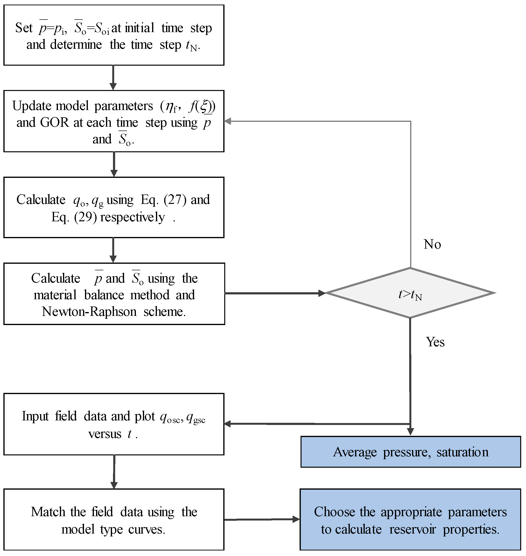
2.4. Work Flow of Two-Phase Flow Analysis

2.4.1. Produced GOR Calculation

The solution derived in the previous section is only for oil phase of horizontal volatile oil wells in fractured carbonate reservoirs, the production of the gas phase is forecast by prediction of the producing GOR, and the method for prediction of the producing GOR is presented in this part.

As stated above, for volatile oil reservoirs, only gas dissolved in the oil phase is considered in this study with ignorance of the oil dissolved in the gas phase. The conventional method used to calculate the producing GOR is based on the assumption that there is a constant relationship between saturation and pressure [32,33,34]. The equation for the producing GOR is expressed by

$$\mathrm{GOR}\left(p_{\mathrm{wf}},S_{\mathrm{owf}}\right)=\frac{q_{\mathrm{gsc}}}{q_{\mathrm{osc}}}=\frac{k_{\mathrm{frg}}}{k_{\mathrm{fro}}}\frac{{\mu }_{\mathrm{o}}{B}_{\mathrm{o}}}{{\mu }_{\mathrm{g}}{B}_{\mathrm{g}}}+R_{\mathrm{s}}$$

(28)

where R_s represents the solution gas-oil ratio; q_gsc represents the surface gas production rate, 10⁴ m³/d; q_osc represents the surface oil production rate, m³/d.

The producing GOR in Equation (28) is a function of pressure and saturation at the wellbore. The bottom-hole flowing pressure is easy to obtain, however, the saturation could not be calculated with analytical models. Therefore, in this approach, an approximate method was proposed to deal with this problem. The saturation dependent parameters in Equation (28) are updated with the average pressure calculated using flowing material balance equations within the investigated area.

The equation for the producing GOR can be rewritten as

$$\mathrm{GOR}\left(\overline{p},{\overline{S}}_{\mathrm{o}}\right)=\frac{k_{\mathrm{frg}}}{k_{\mathrm{fro}}}\left({\overline{S}}_{\mathrm{o}}\right)\frac{{\mu }_{\mathrm{o}}{B}_{\mathrm{o}}}{{\mu }_{\mathrm{g}}{B}_{\mathrm{g}}}\left(\overline{p}\right)+R_{\mathrm{s}}\left(\overline{p}\right)$$

(29)

where GOR represents the producing gas-oil ratio, m³/m³; $k_{\mathrm{fro}}\left({\overline{S}}_{\mathrm{o}}\right)$ represents the relative permeability to oil at the average oil saturation; $R_{\mathrm{s}}\left(\overline{p}\right)$ represents the solution gas at average pressure.

To calculate the average saturation and pressure in Equation (29), the nonlinear equations must be solved iteratively for the oil and gas phases respectively. In the following, a coupled flowing material balance technique is developed to forecast oil and gas production.

2.4.2. Material-Balance Equations

In this section, the detailed derivation of material balance equations for a two-phase system is provided. The basic material balance equation for the oil phase is

$$ROIP=IOIP-N_{\mathrm{p}}$$

(30)

where IOIP is initial oil in place, m³ ROIP is remaining oil in place, m³; N_p is cumulative oil production, m³.

Initial oil in place

$$IOIP=\pi r_{\mathrm{inv}}{}^{2}h\varphi \left(\frac{S_{\mathrm{oi}}}{B_{\mathrm{oi}}}\right)$$

(31)

Remaining oil in place

$$ROIP=\pi r_{\mathrm{inv}}{}^{2}h\varphi \left(\frac{{\overline{S}}_{\mathrm{o}}}{{\overline{B}}_{\mathrm{o}}}\right)$$

(32)

Cumulative oil production

$$N_{\mathrm{p}}={\displaystyle \underset{0}{\overset{t}{\int }}{q}_{\mathrm{o}}\mathrm{d}t}$$

(33)

Substituting Equations (31) through (33) into Equation (30) gives

$$\frac{{\overline{S}}_{\mathrm{o}}}{{\overline{B}}_{\mathrm{o}}}=\frac{S_{\mathrm{oi}}}{B_{\mathrm{oi}}}-\frac{N_{\mathrm{p}}}{\pi r_{\mathrm{inv}}{}^{2}h\varphi }$$

(34)

In this paper, the investigated radius for radial flow is calculated by use of [50]

$$r_{\mathrm{inv}}=0.03248\sqrt{\frac{k_{\mathrm{fi}}}{{\varphi }_{\mathrm{i}}{\mu }_{\mathrm{oi}}{c}_{\mathrm{ti}}}t}$$

(35)

where r_inv represents the investigated radius, m; k_fi represents the fracture permeability of dual-porosity media, MPa.

Similarly, the basic material balance equation for gas is

$$RGIP=IGIP-G_{\mathrm{p}}$$

(36)

where IGIP is initial gas in place, 10⁴ m³; RGIP is remaining gas in place, 10⁴ m³; G_p is cumulative gas production, 10⁴ m³.

Initial gas in place

$$IGIP=\pi r_{\mathrm{inv}}{}^{2}h\varphi \left(\frac{S_{\mathrm{gi}}}{B_{\mathrm{gi}}}+\frac{R_{\mathrm{si}}{S}_{\mathrm{oi}}}{B_{\mathrm{oi}}}\right)$$

(37)

Remaining gas in place

$$RGIP=\pi r_{\mathrm{inv}}{}^{2}h\varphi \left(\frac{{\overline{S}}_{\mathrm{g}}}{{\overline{B}}_{\mathrm{g}}}+\frac{{\overline{R}}_{\mathrm{s}}{\overline{S}}_{\mathrm{o}}}{{\overline{B}}_{\mathrm{o}}}\right)$$

(38)

Cumulative gas production

$$G_{\mathrm{p}}={\displaystyle \underset{0}{\overset{t}{\int }}{q}_{\mathrm{g}}\mathrm{d}t}$$

(39)

Substituting Equations (37) through (39) into Equation (36), one can obtain

$$\left(\frac{{\overline{S}}_{\mathrm{g}}}{{\overline{B}}_{\mathrm{g}}}+\frac{{\overline{R}}_{\mathrm{s}}{\overline{S}}_{\mathrm{o}}}{{\overline{B}}_{\mathrm{o}}}\right)=\left(\frac{S_{\mathrm{gi}}}{B_{\mathrm{gi}}}+\frac{R_{\mathrm{si}}{S}_{\mathrm{oi}}}{B_{\mathrm{oi}}}\right)-\frac{G_{\mathrm{p}}}{\pi r_{\mathrm{inv}}{}^{2}h\varphi }$$

(40)

The saturation relation equation is expressed by

$${\overline{S}}_{\mathrm{g}}+{\overline{S}}_{\mathrm{o}}=1$$

(41)

Combining Equation (34) with Equation (40) and Equation (41) yields that

$$f\left(\overline{p}\right)=\frac{1}{{\overline{B}}_{\mathrm{g}}}+\left({\overline{R}}_{\mathrm{s}}-\frac{{\overline{B}}_{\mathrm{o}}}{{\overline{B}}_{\mathrm{g}}}\right)m_1-m_2$$

(42)

In which

$$m_1=\left(\frac{S_{\mathrm{oi}}}{B_{\mathrm{oi}}}\right)-\frac{N_{\mathrm{p}}}{\pi r_{\mathrm{inv}}{}^{2}h\varphi }$$

(43)

$$m_2=\left(\frac{S_{\mathrm{gi}}}{B_{\mathrm{gi}}}+\frac{R_{\mathrm{si}}{S}_{\mathrm{oi}}}{B_{\mathrm{oi}}}\right)-\frac{G_{\mathrm{p}}}{\pi r_{\mathrm{inv}}{}^{2}h\varphi }$$

(44)

where S_oi and S_gi are the saturations of oil and gas at initial pressure respectively; B_oi and B_gi are the formation volume factors of oil and gas at initial pressure respectively; R_si is the solution gas oil ratio at initial pressure; ${\overline{S}}_{\mathrm{g}}$ and ${\overline{S}}_{\mathrm{o}}$ are the saturations of oil and gas at average pressure, respectively; ${\overline{B}}_{\mathrm{o}}$ and ${\overline{B}}_{\mathrm{g}}$ are the formation volume factors of oil and gas at average pressure, respectively.

According to Equation (42), it is easy to deduce that

$$f^{\prime }\left(\overline{p}\right)=-\frac{1}{{\overline{B}}_{\mathrm{g}}{}^2}\frac{\mathrm{d}{B}_{\mathrm{g}}}{\mathrm{d}p}+m_1\left(\frac{\mathrm{d}{\overline{R}}_{\mathrm{s}}}{\mathrm{d}p}-\frac{1}{{\overline{B}}_{\mathrm{g}}}\frac{\mathrm{d}{B}_{\mathrm{o}}}{\mathrm{d}p}+\frac{B_{\mathrm{o}}}{{\overline{B}}_{\mathrm{g}}{}^2}\frac{\mathrm{d}{B}_{\mathrm{g}}}{\mathrm{d}p}\right)$$

(45)

Then average pressures using the Newton-Raphson scheme for Equation (45) is

$${\overline{p}}_{k+1}={\overline{p}}_k-\omega \frac{f\left(\overline{p_k}\right)}{f^{\prime }\left(\overline{p_k}\right)}$$

(46)

where k is the previous time step, and k+1 is the present time step; ω is the iterative coefficient.

2.4.3. History Matching and Production Prediction

This section provides a flow chart for two-phase history matching and production forecasting with the proposed semi-analytical method. The procedure for estimation of oil and gas production rate and history matching is shown in Figure 2. To conduct history matching and production prediction with the new method successfully, the reliability of model inputs such as reservoir parameters, relative permeability curves, fluid properties, and field data are very significant and should be checked carefully before being used in the model. The production is calculated with the semi-analytical model step by step, and the time increment is given by one day in accordance with the production data. Firstly, the initial average pressure and average saturation are used to calculate the production of the oil phase with Equation (27). The output of the gas phase is forecast with the producing GOR (Equation (29)). The average pressure and saturation within the investigated area are calculated with the flowing material balance equation. Calculations are then repeated for this time step using the Newton–Raphson scheme (Equation (46)). Thus, nonlinear parameters and GOR are updated with the average pressure and saturation at each time step. After that, the production rate curves of oil and gas phases using the proposed model are employed to match the field data. In this paper, we adopted the nonlinear least-square curve fitting method to conduct field data matching by using the semi-analytical method.

3. Results and Discussion

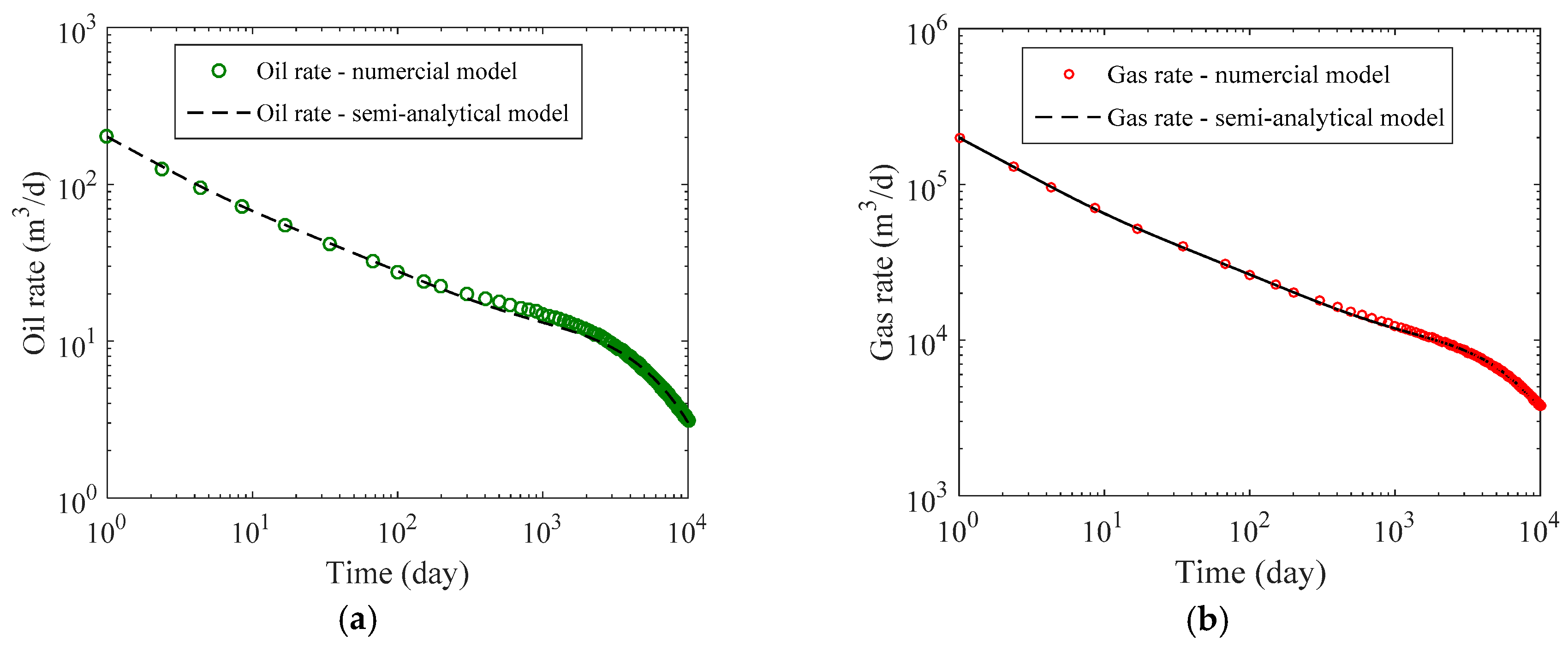
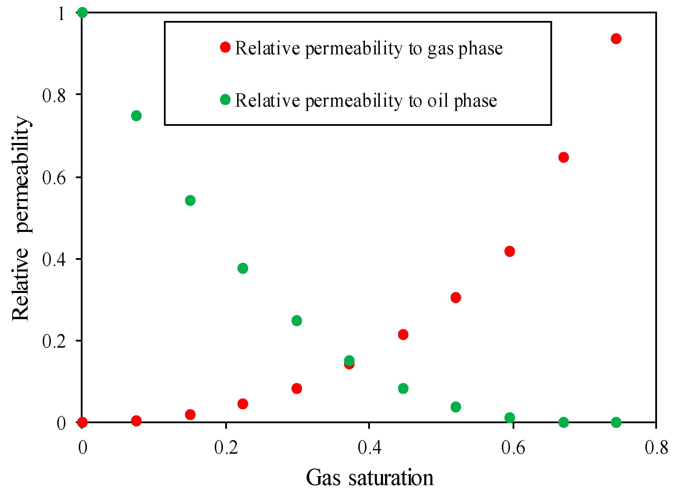
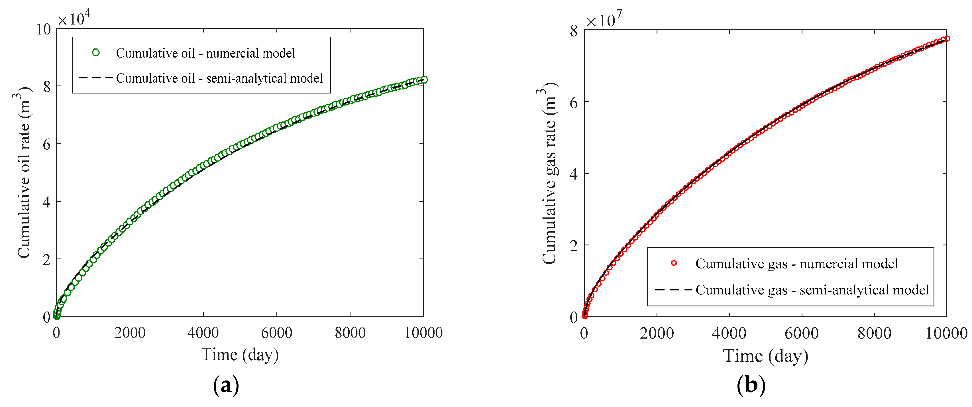
3.1. Model Verification

The proposed semi-analytical method is benchmarked against the commercial simulator Eclipse. A numerical model is built to simulate the two-phase flow of the horizontal volatile oil well. The input parameters for the semi-analytical and numerical model are identical, in which, the horizontal well has a wellbore length of 500 m and is located in the center of the formation. The reservoir diameter and thickness are 880 m and 38 m respectively. The initial reservoir pressure is 24.48 MPa and the bottom-hole pressure is fixed at 6 MPa during the production periods. The basic reservoir, horizontal well, and fluid properties are listed in

Table 1. Parameters used for validation case.

Parameters	Symbol	Unit	Value
Wellbore radius	r	m	0.07
Formation thickness	h	m	38
Matrix porosity	ϕM	Dimensionless	0.1
Horizontal permeability	kh	mD	0.25
Perpendicular permeability	kv	mD	0.25
Permeability modulus	γ	MPa−1	2.2 × 10−3
Rock compressibility	Ct	MPa−1	1.0 × 10−4
Horizontal wellbore length	L	m	500
Perpendicular distance of horizontal well	zw	m	19
Radial distance of external boundary	re	m	880
Initial water saturation	Swi	Dimensionless	0.15
Oil API gravity	/	Dimensionless	40
Reservoir temperature	T	K	323.15
Initial reservoir pressure	pi	MPa	24.48
Bottom-hole pressure	pwf	MPa	6
Bubble point pressure	pb	MPa	22.34

. The initial pressure of the formation is higher than the bubble point of fluids, so the primary phase in the reservoir is the oil phase. In this case, the oil is assumed to be live oil, and the gas is assumed to be dead gas. The fluid properties and relative permeability curves used as input for the semi-analytical and numerical model are shown in Figure 3 and Figure 4 respectively.

Figure 5 and Figure 6 show the comparison of production rate and cumulative production between the semi-analytical method and the numerical simulation. As shown, a good match between the semi-analytical model and the numerical simulation in both flow rate and cumulative production is obtained. The matching error between these two methods for oil production rate and cumulative oil production is less than 2%, which can be seen in Figure 5a and Figure 6a. For the gas production rate and cumulative gas production in Figure 5b and Figure 6b, the matching errors are 3% and 5% respectively. The matching error of the gas production rate and cumulative gas production is higher than the oil phase. This is because the PVT properties of the gas phase are sensitive to the pressure, but less sensitive for the oil phase. Meanwhile, to characterize the pressure sensitive PVT properties, the pseudo-pressure concept is applied in this paper. Although there is a slight mismatch in gas production rate and cumulative gas production, the error is appropriate for engineering purposes (less than 10%). Therefore, the proposed semi-analytical method can accurately simulate the two-phase flow behavior of horizontal volatile oil wells in fractured carbonate reservoirs.

3.2. Sensitivity Analysis

After validation, the influences of some critical parameters on gas and oil production performance are analyzed with the semi-analytical model.

Table 2. Basic parameters used for the sensitivity analysis.

Parameters	Symbol	Unit	Value
Wellbore radius	r	m	0.07
Matrix porosity	ϕM	Dimensionless	0.108
Rock compressibility	Ct	MPa−1	1.0 × 10−4
Perpendicular distance of horizontal well	zw	m	16
Initial water saturation	Swi	Dimensionless	15
Oil API gravity	/	Dimensionless	40
Reservoir temperature	T	K	323.15
Initial reservoir pressure	pi	MPa	26.48
Bottom-hole pressure	pwf	MPa	6
Bubble point pressure	pb	MPa	22.34
Perpendicular permeability	kv	mD	0.25

shows the input parameters used for the sensitivity analysis.

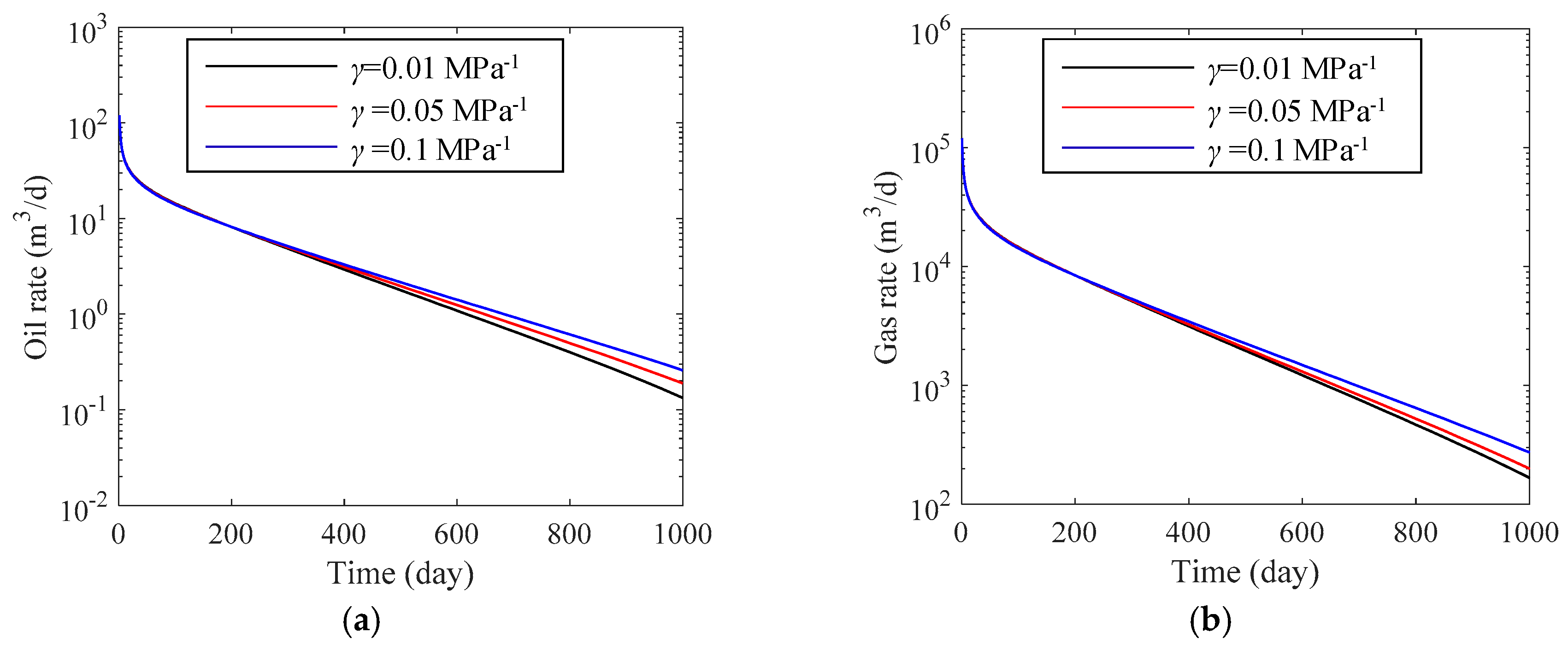
3.2.1. Permeability Stress Sensitivity of Fracture

The permeability stress sensitivity of the fracture is expected to have a significant influence on the production performance in fractured carbonate reservoirs. Therefore, the permeability is evaluated with the average pressure calculated by using flowing material balance equations within the investigated area, which is expressed by

$$k_{\mathrm{f}}=k_{\mathrm{fi}}{e}^{\gamma \left(p_{\mathrm{f}}-p_{\mathrm{i}}\right)}$$

(47)

where γ represents the permeability modulus, MPa⁻¹.

Figure 7 shows the influence of permeability stress sensitivity on production performance. One can see that permeability stress sensitivity affects all production periods, especially in the late period. As the permeability modulus increases, the production rate of both the oil and gas phases decreases greatly during the first year. However, those cases with stronger stress sensitivity have a higher production rate int the late period. This is because the fluid flow will be difficult and more oil and gas are left in the reservoir with the increase of the permeability modulus. The stress-sensitivity reflects the damage of the permeability and a stronger stress-sensitivity will increase the damage of the permeability. Consequently, the permeability stress sensitivity of the fracture decreases the cumulative production.

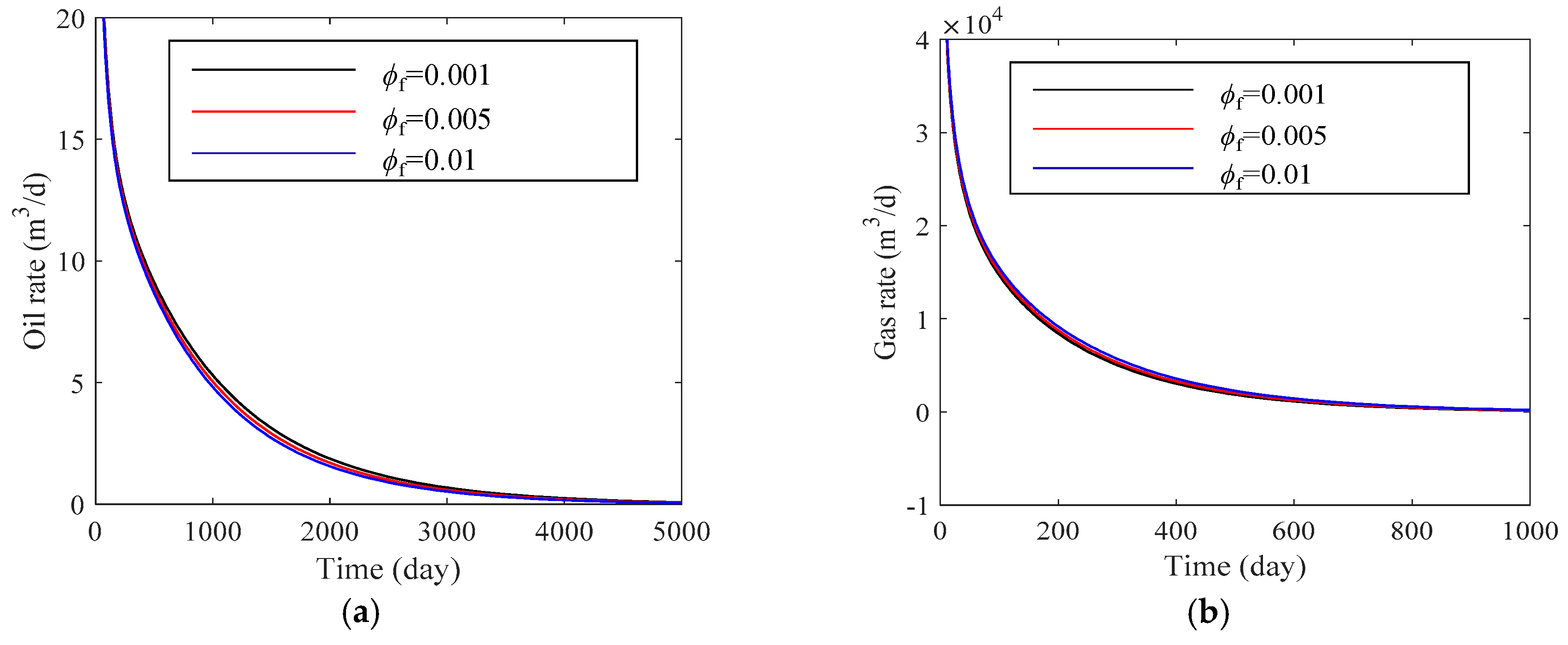
3.2.2. Fracture Porosity

Figure 8 shows the influence of the fracture porosity on the oil and gas production rate calculated by the semi-analytical model. It can be seen from Figure 8 that the production rate increases with the increase of the fracture porosity during the early and intermediate flow periods. However, the fracture porosity has little effect on the late production period. This is because the fracture porosity reflects the relative capacity of the fluid stored in the fracture system, a bigger fracture porosity is the response of the relative abundant reserves in the fracture system. The production drop should decrease to maintain the constant bottom-hole pressure of the production well when increasing the fracture porosity. Meanwhile, compared with the fracture storing capacity of the affected region of the pressure wave, the increment of fracture storing capacity could be neglected during the late flow period. That is the reason why the fracture porosity has little effect on the late production period.

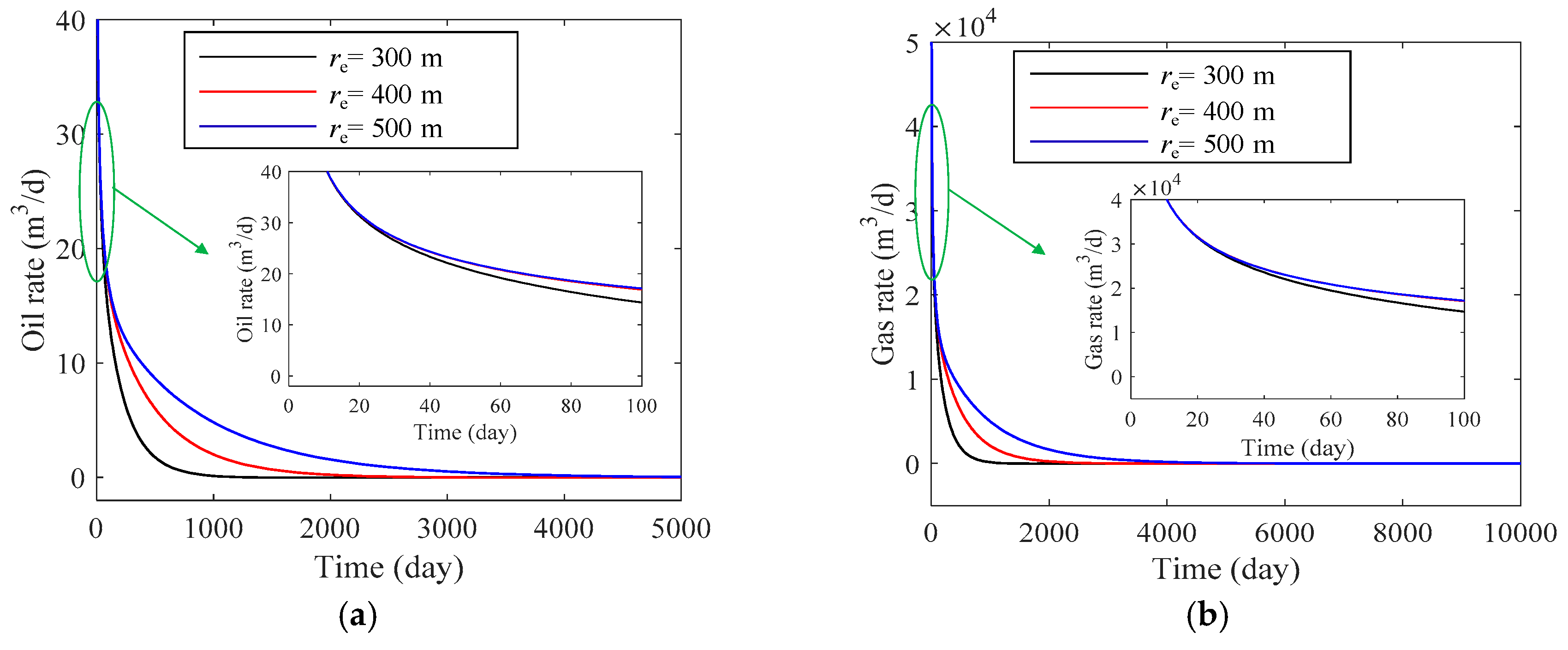
3.2.3. Radial Distance of External Boundary

Figure 9 shows the effect of the radial distance of the external boundary on the production rate. The value of the radial distance of the external boundary reflects the size of the drainage area. The results in Figure 9 indicate that the smaller the drainage area, the faster the production rate declined. As the radial distance of the external boundary increases, the production rates of both oil and gas phases increase greatly during the early and intermediate flow periods. This is because when the radial distance of the external boundary increases, the time of the external boundary response will be delayed, so the production drop should decrease to maintain the constant bottom-hole pressure of the well. In addition, the radial distance of the external boundary has little effect on the production rate before 40 days as shown in Figure 9. This is because the pressure wave is just propagated to the top and bottom boundary.

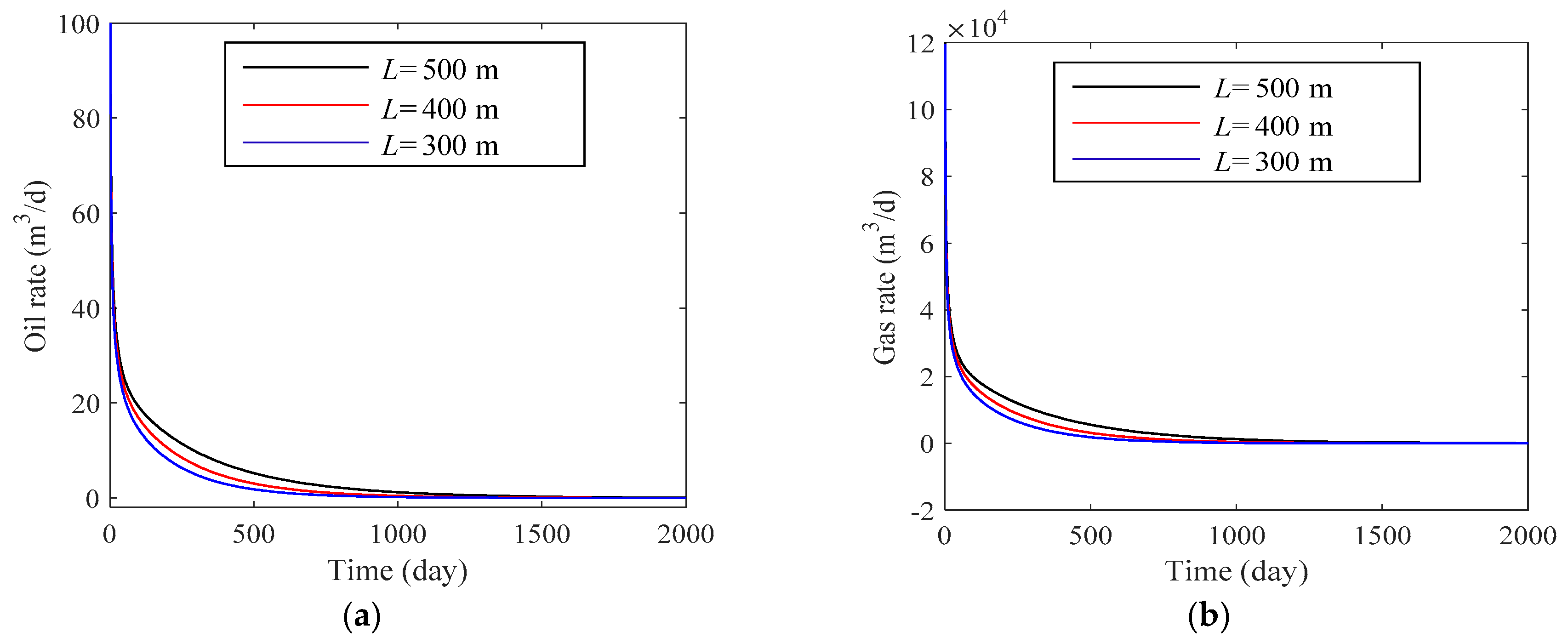
3.2.4. Horizontal Wellbore Length and Reservoir Thickness

Figure 10 and Figure 11 show the effects of horizontal wellbore length and reservoir thickness on the production dynamics of a horizontal well in fractured carbonate volatile oil reservoirs, respectively. As shown in Figure 10, the horizontal wellbore length affects the production rate during the whole process. Increasing the horizontal wellbore length will lead to an increase in production rate, particularly in the intermediate production period. It can be seen from Figure 11 that a greater reservoir thickness will generate a higher production rate during the early production periods. This is because the pressure drop will increase and the pressure wave needs more time to propagate to the closed boundary when increasing the value of the reservoir thickness.

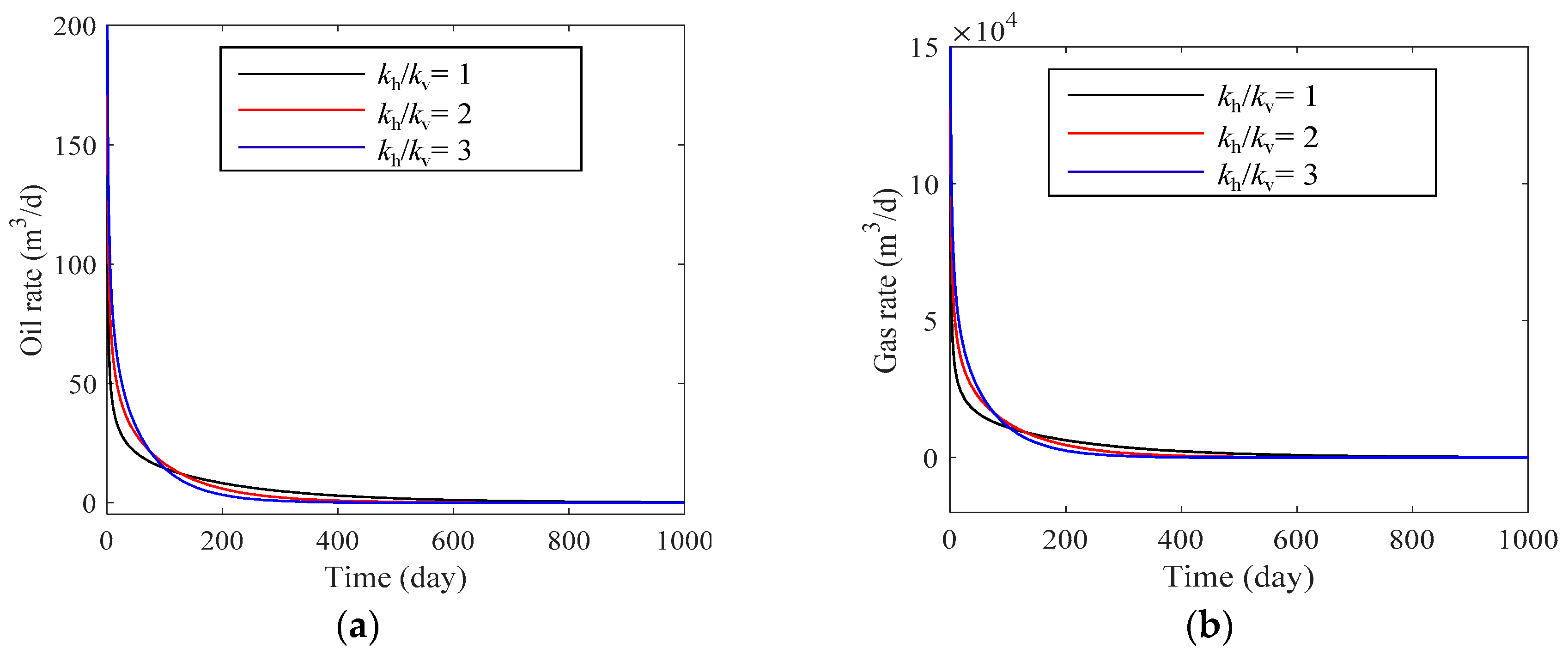
3.2.5. Ratio of Horizontal Permeability to Perpendicular Permeability

Figure 12 shows the effect of the ratio of horizontal permeability to perpendicular permeability on the oil and gas production rate. It can be observed that a larger k_h/k_v will result in a higher production rate during the early production periods. This is because the fluid flow will be more difficult in the vertical direction and the pressure drop will increase when increasing k_h/k_v, so the larger the k_h/k_v, the later the pressure wave propagates to the top and bottom boundary, and the higher the production rate will be.

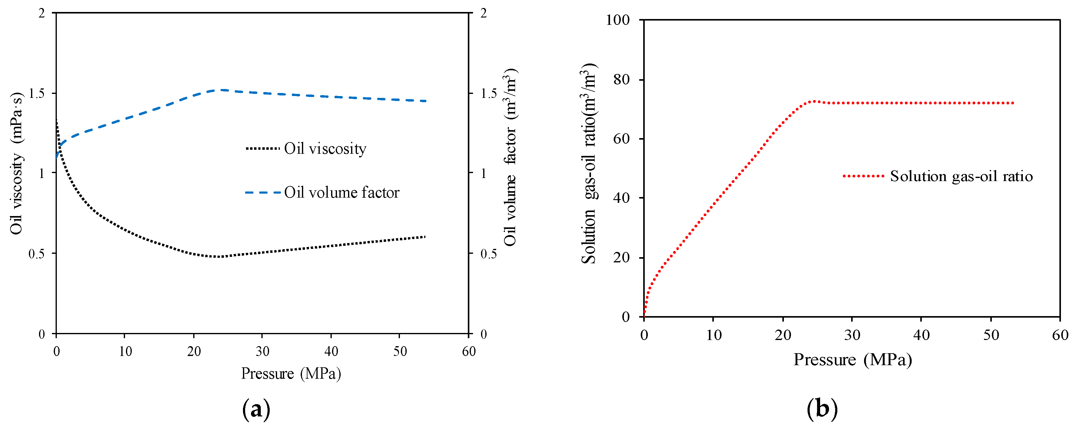
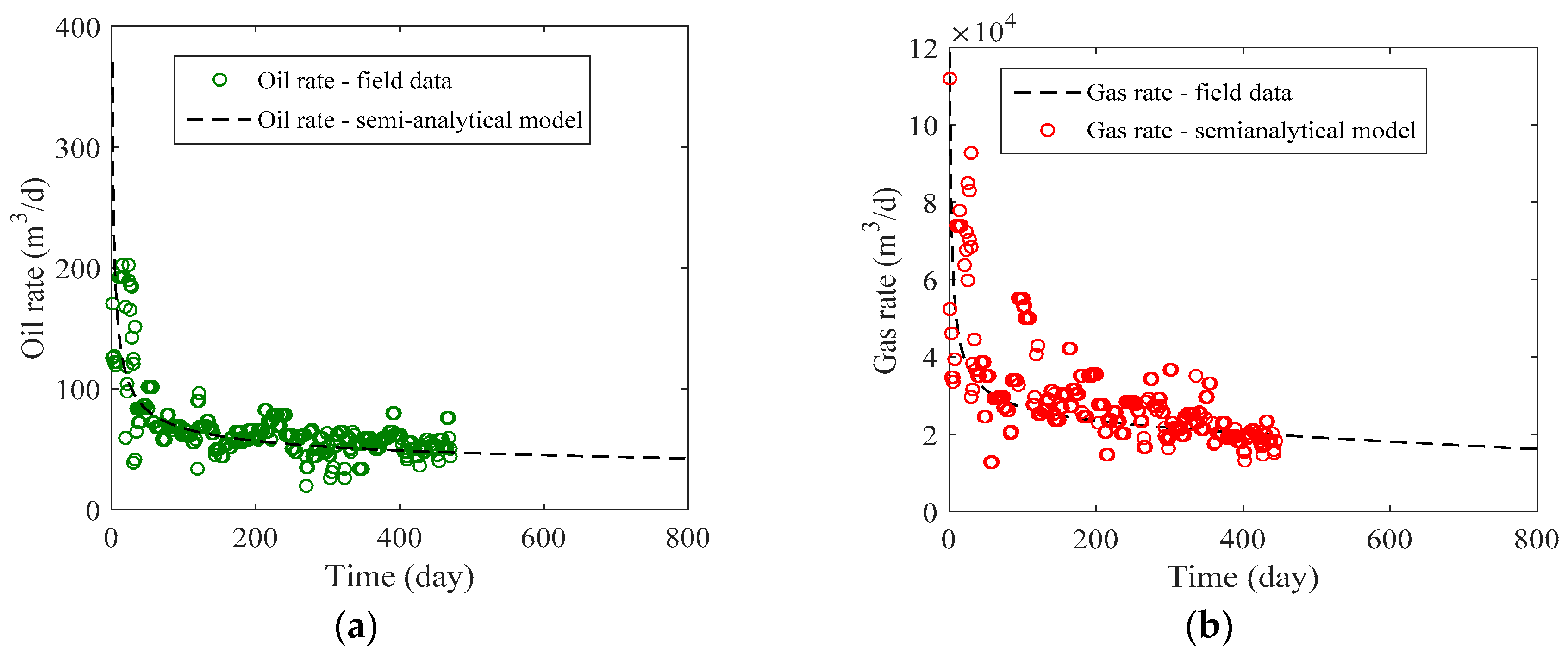
3.3. Methodology Application: A Case Study

The accuracy of the proposed semi-analytical model for forecasting was demonstrated in the previous sections. In this section, to test the practical applicability of the semi-analytical method, field data obtained from a horizontal well completed in a fractured carbonate volatile oil reservoir in the eastern Pre-Caspian basin is analyzed.

Table 3. Basic input parameters for field case.

Parameters	Symbol	Unit	Value
Wellbore radius	r	m	0.07
Formation thickness	h	m	24
Matrix porosity	ϕM	Dimensionless	0.148
Rock compressibility	Ct	MPa−1	1.0 × 10−4
Perpendicular distance of horizontal well	zw	m	12
Initial water saturation	Swi	Dimensionless	0.15
Oil API gravity	/	Dimensionless	40
Reservoir temperature	T	K	358
Initial reservoir pressure	pi	MPa	24.8
Bottom-hole pressure	pwf	MPa	6
Bubble point pressure	pb	MPa	22.34

provides the critical parameters of formation, fracture, and production used for this field case. Figure 13 shows the history matching results for the field case using the proposed semi-analytical method. A satisfactory history matching result is obtained and the final production rate match of the oil phase is less than 3% and within 5% for the gas phase. Although the match to the gas phase appears to be poorer, the match is acceptable for engineering purposes (within 10%).

The interpreted parameters using the semi-analytical model are presented in

Table 4. Main interpreted parameters for field case.

Interpreted Parameters	Symbol	Unit	Value
Fracture permeability	kh	mD	2.6
Permeability modulus	γ	MPa−1	0.014
Fracture porosity	ϕf	Dimensionless	0.005
Horizontal wellbore length	L	m	580
Radial distance of external boundary	re	m	850

. The results show that the interpreted horizontal wellbore length and fracture permeability are 580 m and 2.6 mD respectively, which is in accordance with the actual condition. Besides, the interpretation result of the permeability modulus is 0.014 MPa⁻¹, which indicates that the fracture has a strong permeability stress sensitivity. Moreover, the interpreted fracture porosity is 0.005, which implies that the fracture system has a relatively stronger storage capability. These interpreted parameters are all reasonable and conform to the understanding of horizontal volatile oil wells in fractured carbonate reservoirs.

4. Conclusions

Although not as versatile as numerical simulators, the proposed semi-analytical method is indeed a practical method for simulating two-phase flow and making forecasts for horizontal volatile oil wells. The results of this investigation show that the horizontal wellbore length, reservoir thickness, reservoir anisotropy, stress-dependency of fracture permeability, fracture porosity, and exterior boundary all play a most significant role in production performance. Permeability stress sensitivity plays an important role over the whole production periods. As the permeability modulus increases, the production rate of both the oil and gas phases decreases greatly during the early production stage, but those cases with stronger stress sensitivity have a higher production rate in the late period. In addition, increasing the fracture porosity and the exterior boundary will increase the production rate in the early and intermediate production periods. Moreover, greater horizontal wellbore length will lead to a higher production rate, particularly during the intermediate production period. Finally, a field example from the eastern Pre-Caspian basin was used to show the practicability of the new method. Good history matching results were observed and satisfied interpreted parameters obtained, which reveals the new method’s reliability in analyzing two-phase production data of horizontal volatile oil wells in fractured carbonate reservoirs.

The main contribution of this paper is the provision of a semi-analytical method to accurately analyze production data and make reliable forecasts for horizontal volatile oil wells in fractured carbonate reservoirs.

References

1. Thiebot, B.M.; Sakthikumar, S.S. Cycling fractured reservoirs containing volatile oil: Laboratory investigation of the performance of lean gas or nitrogen injection. In Proceedings of the Middle East Oil Show, Manama, Bahrain, 16–19 November 1991. [Google Scholar]
2. Ghorbani, D.; Kharrat, R. Fluid characterization of an Iranian carbonate oil reservoir using different PVT packages. In Proceedings of the Asia Pacific Oil and Gas Conference and Exhibition, Jakarta, Indonesia, 17–19 April 2000. [Google Scholar]
3. Kang, Z.; Wu, Y.-S.; Li, J.; Zhang, J.; Wang, G. Modeling multiphase flow in naturally fractured vuggy petroleum reservoirs. In Proceedings of the SPE Annual Technical Conference and Exhibition, San Antonio, TX, USA, 24–27 September 2006. [Google Scholar] [CrossRef]
4. Gringarten, A.C.; Ogunrewo, O.; Uxukbayev, G. Assessment of individual skin factors in gas condensate and volatile oil wells. In Proceedings of the SPE EUROPEC/EAGE Annual Conference and Exhibition, Vienna, Austria, 23–26 May 2011. [Google Scholar] [CrossRef]
5. Poon, D.C. Decline curves for predicting production performance from horizontal wells. J. Can. Petrol. Technol. 1991, 30, 77–81. [Google Scholar] [CrossRef]
6. Ozkan, E. Analysis of horizontal-well responses: Contemporary vs. conventional. SPE Reserv. Eval. Eng. 2001, 4, 260–269. [Google Scholar] [CrossRef]
7. Hashemi, A.; Nicolas, L.M.; France, G.D.; Gringarten, A.C. Well test analysis of horizontal wells in gas-condensate reservoirs. SPE Reserv. Eval. Eng. 2006, 9, 86–99. [Google Scholar] [CrossRef]
8. Hagoort, J. A simplified analytical method for estimating the productivity of a horizontal well producing at constant rate or constant pressure. J. Petrol. Sci. Eng. 2009, 64, 77–87. [Google Scholar] [CrossRef]
9. Nie, R.-S.; Meng, Y.-F.; Jia, Y.-L.; Zhang, F.-X.; Yang, X.-T.; Niu, X.-J. Dual porosity and dual permeability modeling of horizontal well in naturally fractured reservoir. Transp. Porous Med. 2012, 92, 213–235. [Google Scholar] [CrossRef]
10. Nie, R.-S.; Jia, Y.-L.; Meng, Y.-F.; Wang, Y.; Yuan, J.; Xu, W. New type curves for modeling productivity of horizontal well with negative skin factors. SPE Reserv. Eval. Eng. 2012, 15, 486–497. [Google Scholar] [CrossRef]
11. Wu, Y.-H.; Cheng, L.-S.; Huang, S.-J.; Jia, P.; Zhang, J.; Lan, X.; Huang, H.-L. A practical method for production data analysis from multistage fractured horizontal wells in shale gas reservoirs. Fuel 2016, 186, 821–829. [Google Scholar] [CrossRef]
12. Jia, P.; Cheng, L.-S.; Clarkson, C.R. A Laplace-domain hybrid model for representing flow behavior of multifractured horizontal wells communicating through secondary fractures in unconventional reservoirs. SPE J. 2017, 22, 1856–1876. [Google Scholar] [CrossRef]
13. Warren, J.E.; Root, P.J. The behavior of naturally fractured reservoirs. SPE J. 1963, 228, 245–255. [Google Scholar] [CrossRef]
14. Kazemi, H. Pressure transient analysis of naturally fractured reservoirs with uniform fracture distribution. SPE J. 1969, 11, 451–462. [Google Scholar] [CrossRef]
15. De Swaan, O.A. Analytical solutions for determining naturally fractured reservoir properties by well testing. SPE J. 1976, 16, 117–122. [Google Scholar] [CrossRef]
16. Ozkan, E.; Ohaeri, U. Unsteady flow to a well produced at a constant pressure in a fractured reservoir. SPE Form. Eval. 1987, 2, 186–200. [Google Scholar] [CrossRef]
17. Al-Ghamdi, A.; Ershaghi, I. Pressure transient analysis of dually fractured reservoirs. SPE J. 1996, 1, 93–100. [Google Scholar] [CrossRef]
18. Arps, J.J. Analysis of decline curves. Trans. AIME 1945, 160, 228–247. [Google Scholar] [CrossRef]
19. Shea, G.B.; Higgins, R.V.; Lechtenberg, H.J. Decline and forecast studies based on performances of selected California oilfields. J. Pet. Technol. 1964, 16, 959–965. [Google Scholar] [CrossRef]
20. Masoner, L.O. A decline analysis technique incorporating corrections for total fluid rate changes. SPE Reserv. Eval. Eng. 1996, 2, 533–541. [Google Scholar] [CrossRef]
21. Hsieh, F.; Vega, C.; Vega, L. Reserves estimation using a PC decline analysis program. J. Can. Petrol. Technol. 2001, 40, 13–15. [Google Scholar] [CrossRef]
22. Gaskari, R.; Mohaghegh, S.; Jalali, J. An integrated technique for production data analysis with application to mature fields. SPE Prod. Oper. 2007, 22, 403–416. [Google Scholar] [CrossRef]
23. Ilk, D.; Rushing, J.A.; Perego, A.D.; Blasingame, T.A. Exponential vs. hyperbolic decline in tight gas sands: Understanding the origin and implications for reserve estimates using Arps’ decline curves. In Proceedings of the SPE Annual Technical Conference and Exhibition, Denver, CO, USA, 21–24 September 2008. [Google Scholar]
24. Wilson, A. Comparison of empirical and analytical methods for production forecasting. J. Pet. Technol. 2015, 67, 133–136. [Google Scholar] [CrossRef]
25. Wu, Y.-S. Numerical simulation of single-phase and multiphase non-Darcy flow in porous and fractured reservoirs. Transp. Porous Med. 2002, 49, 209–240. [Google Scholar] [CrossRef]
26. Gill, H.; Issaka, M.B. Pressure transient behavior of horizontal and slant wells intersecting a high-permeability layer. In Proceedings of the SPE Middle East Oil and Gas Show and Conference, Manama, Bahrain, 11–14 March 2007. [Google Scholar]
27. Mahmoud, M.A.; Nasr-El-Din, H.A. Challenges during shallow and deep carbonate reservoirs stimulation. J. Energy Resour. Technol. 2012, 137, 8. [Google Scholar] [CrossRef]
28. Rao, X.; Cheng, L.-S.; Cao, R.-Y.; Jiang, J.-M.; Fang, S.-D.; Jia, P.; Wang, L. Engineering analysis with boundary elements a novel green element method based on two sets of nodes. Eng. Anal. Bound. Elem. 2018, 91, 124–131. [Google Scholar] [CrossRef]
29. Rao, X.; Cheng, L.-S.; Cao, R.-Y.; Jiang, J.-M.; Li, N.; Fang, S.-D.; Wang, L. A novel green element method by mixing the idea of the finite difference method. Eng. Anal. Bound. Elem. 2018, 95, 238–247. [Google Scholar] [CrossRef]
30. Perrine, R.L. Analysis of pressure-buildup curves. In Proceedings of the Drilling and Production Practice, New York, NY, USA, 1 January 1956. [Google Scholar]
31. Martin, J.C. Simplified equations of flow in gas drive reservoirs and the theoretical foundation of two-phase pressure buildup analyses. AIME 1959, 216, 309–311. [Google Scholar]
32. Fetkovich, M.J. The isochronal testing of oil wells. In Proceedings of the Fall Meeting of the Society of Petroleum Engineers of AIME, Las Vegas, NV, USA, 30 September–3 October 1973. [Google Scholar]
33. Raghavan, R. Well test analysis: Wells producing by solution gas drive. SPE J. 1976, 16, 196–208. [Google Scholar] [CrossRef]
34. Camacho-V, R.G.; Raghavan, R. Performance of wells in solution-gas-drive reservoirs. SPE Form. Eval. 1989, 4, 611–620. [Google Scholar] [CrossRef]
35. Ozkan, E.; Raghavan, R. New solutions for well-test-analysis problems: Part 1—Analytical considerations. SPE Form. Eval. 1991, 6, 359–368. [Google Scholar] [CrossRef]
36. Ozkan, E.; Raghavan, R. New solutions for well-test-analysis problems: Part 2—Computational considerations and applications. SPE Form. Eval. 1991, 6, 369–378. [Google Scholar] [CrossRef]
37. Ng, M.G.; Aguilera, R. Well test analysis of horizontal wells in bounded naturally fractured reservoirs. J. Can. Petrol. Technol. 1999, 38, 20–24. [Google Scholar] [CrossRef]
38. O’Sullivan, M.J. A similarity method for geothermal well test analysis. Water Resour. Res. 1981, 17, 390–398. [Google Scholar] [CrossRef]
39. Bøe, A.; Skjaeveland, S.; Whitson, C. Two-phase pressure test analysis. SPE Form. Eval. 1989, 4, 604–610. [Google Scholar] [CrossRef]
40. Kissling, W.; McGuinness, M.; McNabb, A. Analysis of one-dimensional horizontal two-phase flow in geothermal reservoirs. Transp. Porous Med. 1992, 7, 223–253. [Google Scholar] [CrossRef]
41. Ayala, L.F.; Kouassi, J.P. The similarity theory applied to the analysis of two-phase flow in gas-condensate reservoirs. Energy Fuel 2007, 21, 1592–1600. [Google Scholar] [CrossRef]
42. Zhang, M.; Ayala, L.F. Analytical study of constant gas–oil-ratio behavior as an infinite-acting effect in unconventional two-phase reservoir systems. SPE J. 2016, 22, 1–11. [Google Scholar] [CrossRef]
43. Jia, P.; Cheng, L.-S.; Huang, S.-J. A semi-analytical model for the flow behavior of naturally fractured formations with multi-scale fracture networks. J. Hydrol. 2016, 537, 208–220. [Google Scholar] [CrossRef]
44. Jia, P.; Cheng, L.-S.; Clarkson, C.R. Flow behavior analysis of two-phase flowback and early-time production from hydraulically-fractured shale gas wells using a hybrid numerical/analytical model. Int. J. Coal. Geol. 2017, 180, 14–31. [Google Scholar] [CrossRef]
45. Li, Y.; Zuo, W.; Yu, W.; Chen, Y. A fully three dimensional semi-analytical model for shale gas reservoirs with hydraulic fractures. Energies 2018, 11, 436. [Google Scholar] [CrossRef]
46. Clarkson, C.R.; Qanbari, F. A semi-analytical forecasting method for unconventional gas and light oil wells: A hybrid approach for addressing the limitations of existing empirical and analytical methods. SPE Reserv. Eval. Eng. 2014, 18, 260–263. [Google Scholar] [CrossRef]
47. Clarkson, C.R.; Qanbari, F. An approximate semi-analytical two-phase forecasting method for multifractured tight light-oil wells with complex fracture geometry. J. Can. Petrol. Technol. 2015, 54, 489–508. [Google Scholar] [CrossRef]
48. Guo, J.-C.; Nie, R.-S.; Jia, Y.-L. Unsteady-state diffusion modeling of gas in coal matrix for horizontal well production. AAPG Bull. 2014, 98, 1669–1697. [Google Scholar] [CrossRef]
49. Stehfest, H. Numerical inversion of Laplace transforms. ACM Commun. 1970, 13, 47–49. [Google Scholar] [CrossRef]
50. Kuchuk, F.-J. Radius of investigation for reserve estimation from pressure transient well tests. In Proceedings of the SPE Middle East Oil and Gas Show and Conference, Manama, Bahrain, 15–18 March 2009. [Google Scholar]
Figure 1. Description of the dual-porosity model in this paper: (a) horizontal well-scheme in formation; (b) dual-porosity model flow scheme; (c) dual-porosity model with spherical matrix.
Energies 11 02700 g001
Figure 2. Flowchart of history matching procedure using the proposed semi-analytical method.
Energies 11 02700 g002
Figure 3. PVT properties used as input for the semi-analytical and numerical model: (a) oil volume factor and viscosity curves; (b) solution gas-oil ratio curve.
Energies 11 02700 g003
Figure 4. Relative permeability curve used as input for the semi-analytical and numerical model.
Energies 11 02700 g004
Figure 5. Results comparison of production rate between numerical simulation and the semi-analytical method for validation case: (a) log-log plot of oil production rate; (b) log-log plot of gas production rate.
Energies 11 02700 g005
Figure 6. Results comparison of cumulative production between numerical simulation and the semi-analytical method for validation case: (a) Cartesian plot of cumulative oil production; (b) Cartesian plot of cumulative gas production.
Energies 11 02700 g006
Figure 7. Influence of permeability stress sensitivity of fracture on production rate: (a) influence of permeability stress sensitivity on oil production rate; (b) influence of permeability stress sensitivity on gas production rate.
Energies 11 02700 g007
Figure 8. Effect of fracture porosity on production rate: (a) effect of fracture porosity on oil production rate; (b) effect of fracture porosity on gas production rate.
Energies 11 02700 g008
Figure 9. Effect of radial distance of external boundary on production rate: (a) effect of radial distance of external boundary on oil production rate; (b) effect of radial distance of external boundary on gas production rate.
Energies 11 02700 g009
Figure 10. Effect of length of horizontal well section on production rate: (a) effect of length of horizontal well section on oil production rate; (b) effect of length of horizontal well section on gas production rate.
Energies 11 02700 g010
Figure 11. Effect of reservoir thickness on production rate: (a) effect of reservoir thickness on oil production rate; (b) effect of reservoir thickness on gas production rate.
Energies 11 02700 g011
Figure 12. Effect of permeability ratio on production rate: (a) effect of permeability ratio on oil production rate; (b) effect of permeability ratio on gas production rate.
Energies 11 02700 g012
Figure 13. History matching results for field case: (a) Cartesian plot of oil production; (b) Cartesian plot of gas production.
Energies 11 02700 g013