Article

Cooling Process Analysis of a 5-Drum System for Radioactive Waste Processing

1
Thermal Engineering Group, Energy Engineering Department, School of Engineering, Universidad de Sevilla, Camino de los Descubrimientos, s/n, 41092 Sevilla, Spain
2
NUSIM S.A. c/Balbino Marrón, 8, Pl. 6, 41018 Sevilla, Spain
*
Author to whom correspondence should be addressed.
Energies 2018, 11(10), 2689; https://doi.org/10.3390/en11102689
Submission received: 7 September 2018 / Revised: 4 October 2018 / Accepted: 8 October 2018 / Published: 9 October 2018

Abstract

:
A cooling system design for the processing of radioactive waste drums is investigated in this work, with the objective of providing insights for the determination of the air flow rate required to ensure an acceptable slag temperature (323 K or below) after 5 days. A methodology based on both 3D and 2D axisymmetric Computational Fluid Dynamics (CFD) modelling is developed. Transient temperature distributions within the drums in time and space determined by the heat transfer characteristics are studied in detail. A sensitivity analysis is also carried out assuming different physical properties of the radioactive slag. It was found out that for all variations analyzed, the maximum temperature of slag at the end of five days cooling is below 323 K, where the maximum outlet air temperature for a minimum air inlet velocity of 1 m/s is between 320 K and 323 K depending on the radioactive slag properties. When glass-like radioactive slag properties are assumed, the internal heat conduction within the slag is limiting the overall heat transfer, therefore requiring significantly longer cooling times.

1. Introduction

Heat transfer is one of the fundamental aspects to consider for nuclear waste processing and storage, and it has been therefore the objective of many research studies. Nowadays, Computational Fluid Dynamics (CFD) is commonly used for the design and research of the heat transfer processes associated to nuclear power generation, such as reactor cooling, nuclear material rods cooling, and safety issues. Regarding reactor cooling, Weng et al. [1] carried out a CFD investigation of the performance of a special direct vessel injection (DVI) structure for the core cooling system in a 1400 MW pressurized-water reactor. Flow mixing and heat transfer capability in the reactor vessel was analysed under different injection conditions. Maitri et al. [2] developed CFD simulations to later derive linear dynamic models for the cooling control system for a supercritical water cooled reactor (SCWR). Borreani et al. [3] studied different Primary Circulation Pump designs by means of CFD modelling and simulations, for a Lead-cooled Fast Reactor (LFR) within the Generation-IV initiative. Non-conventional axial pumps were investigated, showing that a blade pump presented the best performance in terms of pressure head generated. CFD thermal hydraulic simulations of the moderator tank in a pressure vessel PHWR were carried out by Corzo et al. [4], considering also the heat source by neutron thermalization. The Boussinesq approach was used for high Rayleigh number flow. Park et al. [5] carried out an experimental study on a novel liquid metal fin concept for the prevention of boiling critical heat flux, and their CFD simulations confirmed that heat transfer was improved when the liquid metal was flooded. Şahin et al. [6] presented a CFD study on modular helium reactors, analyzing the effects of the increase in the coolant outlet temperature modifying inlet temperature, flow rate and bypass flow fraction. Simões et al. [7] and Smith et al. [8] focused on the CFD simulation of gas-liquid two-phase flow in pipes, frequently encountered in nuclear applications and essential in predicting the behavior of reactor systems. Iacobides et al. [9] reported alternative strategies for modelling turbulent flow and local heat-transfer coefficients around in-line tube banks, mainly focused on advanced gas-cooled nuclear reactors (AGRs). The suitability and accuracy of wall-resolved large-eddy simulation (LES) and Unsteady Reynolds-Averaged Navier-Stokes (URANS) approaches were examined and compared with experiments. Other cooling fluids such as molten salts were analysed by Shin et al. [10] who carried out both experimental measurements in a scaled-down facility and CFD simulations of the natural circulation on molten salt cooled reactors.
Regarding nuclear material rods cooling, Cong and Zhang [11] investigated the characteristics of bubbles of different sizes in the fuel assembly, which is playing a crucial role in the two-phase flow and heat transfer capacity. The two-phase flow in a fuel assembly was modelled by the Eulerian two-fluid model and the MUltiple SIze Group (MUSIG) model. They found that due to the swirl flow caused by the mixing vane, bubbles can crowd at the heated surface, which may anticipate the occurrence of departure from nucleation boiling. Mixed and forced convection in vertical rod bundles was studied by Sohag et al. [12], and different spacers were evaluated by means of CFD simulations by Chen et al. [13] and Liu et al. [14], focusing on thermal-hydraulic behavior and the influence of the turbulence model used. Experimental measurements and Large Eddy Simulations of the fluid flow through a 37 element CANDU nuclear fuel bundle were presented by Piro et al. [15], reporting a good model results agreement with the experimental measurements of fluid velocity and discussed 3D flow effects such as geometry-induced inter-subchannel mixing, recirculation, swirl or flow separation. Delafontaine et al. [16] also presented an extensive validation of CFD transient fluctuating hydraulics simulations of a fuel rod bundle mock-up with mixing grids in PWR. Also spent fuel pool cooling has been a subject for CFD modeling, as in the work of Hung et al. [17], who developed a three-dimensional two-phase thermal hydraulic model. The importance of appropriate layout of spent fuel arrangement was shown in the simulation results. New heat transfer correlations for the single-phase natural convection were presented.
Regarding safety issues, Liao and Lucas [18] studied the flashing phenomenon, which is relevant to nuclear safety analysis during a loss of coolant accident. It was concluded that a poly-disperse method is necessary for the reliable prediction of the mean bubble size and phase distribution. Yang et al. [19] investigated the circumferential non-uniformity of heat transfer in rod bundles. A three-dimensional model for the cylindrical fuel was introduced in a thermal-hydraulic code to predict circumferential heat transfer non-uniformity in different geometry and flow conditions. Ciparisse et al. [20] studied the dust resuspension risk after a Loss of Vacuum Accident (LOVA) at the International Thermonuclear Experimental Reactor (ITER). The work was carried out by means of a CFD simulation of the beginning of the pressurisation transient. It was identified that a high mobilization risk of the dust was expected on the entire internal surface of the reactor, depending on the reactor scale as higher speeds and greater dust resuspension capacity of the flow is expected in real-scale reactors. Regarding hydrogen distribution during severe accidents, density stratification and its breakup were analysed by Abe et al. [21] both experimentally and by means of CFD simulations, considering the upward buoyant flow pattern as “diffuse” neither pure jet nor pure plume. The temporal evolution of the temperature and hydrogen concentration distributions in the core of the boiling water reactor (BWR) during a severe accident were computed using CFD methods by Valdés-Parada et al. [22]. Many other accident scenarios have been also studied by CFD simulations, such as for the fall-off core barrel assembly [23] or CO2-gas jet into liquid-sodium following a heat exchanger leakage scenario in Sodium Fast Reactors [24].
This trend in the use of CFD for nuclear power generation studies is expected to grow as studies involving safety of nuclear power plants have also increased the after the Fukushima Daiichi nuclear disaster that was caused by a tsunami on 11 March 2011.
CFD is also being used for heat transfer investigation of different nuclear waste processing technologies. Chang et al. [25] investigated the heat flow characteristics and thermal performance of a dry storage cask both experimentally and by CFD simulations. They found that inner flow circulations occur in the flow channel of the cask, affecting the heat dissipation of the dry storage cask. Lee et al. [26] carried out the thermal-fluid flow analysis for a spent fuel storage system using the commercial code FLUENT, defining a porous model to simplify the complex configuration of the fuel assembly. They successfully predict the temperature distributions of the storage cask, and calculated that the maximum calculated temperatures of the spent fuel and the concrete overpack were lower than the allowable values. Lo Frano et al. [27] evaluated the integrity of spent fuel cask under both normal and accident transport conditions. The finite element code ANSYS were used for both steady-state and transient thermal analyses aimed at determining the maximum fuel temperature and the temperatures behaviour into the cask. A similar work was carried out by Xu et al. [28], who developed a finite element model in ANSYS to study the heat transfer mechanisms, defining an equivalent convection coefficient to represent the boundary conditions. Temperature fields were analyzed under normal and accident transport conditions. Tseng et al. [29] also used FLUENT software to investigate the thermal performance of a novel storage system. Conjugate heat transfer coupled with thermal radiation was modelled, and simulation results were used to verify whether the design fulfills the thermal requirements and the temperature limitation of the structure materials. Sanyal et al. [30] performed a CFD thermal design of a transportation cask under fire scenarios, in order to verify the compliance with the guidelines of regulatory bodies. Bullard et al. [31] proposed a new transport cask design, and temperature profiles were determined by two dimensional CFD simulations of conduction, convection, and radiation within the cask. They carried out simulations for different cask designs with smooth or corrugated external surface and various shield thicknesses, finally defining the design that not exceed the limits for both the fuel cladding and outer surface temperatures.
In this work, the thermal and heat transfer characteristics of a nuclear waste processing unit are investigated. The processing unit has the objective of cooling waste material drums, coming from a previous operation that melts the radioactive waste forming a melted slag. The objective of the study is to analyse the cooling system and to provide insights into the design process, as well as the optimization of its operation determining the minimum air flow rate needed in order to ensure a maximum acceptable slag temperature of 323 K after 5 days of cooling. Computational Fluid Dynamics (CFD) has been used for the simulations, following the methods presented in the next sections.
As the heat transfer transient analysis of the entire system is highly complex in terms of CFD computing time, given the different scales in space and time and the consequent spatial and time discretization requirements, a decoupled approach was therefore developed in order to enable the transient cooling analysis. Two different sub-systems were analysed (i.e., the external 3D air flow forced convection around the drums, and secondly the transient conduction heat transfer within the different drum elements, where the coupling interface between both simulations is the external wall of the drums). This approach is required in order to enable the accomplishment of the full transient cooling process in a CFD simulation.

2. Materials and Methods

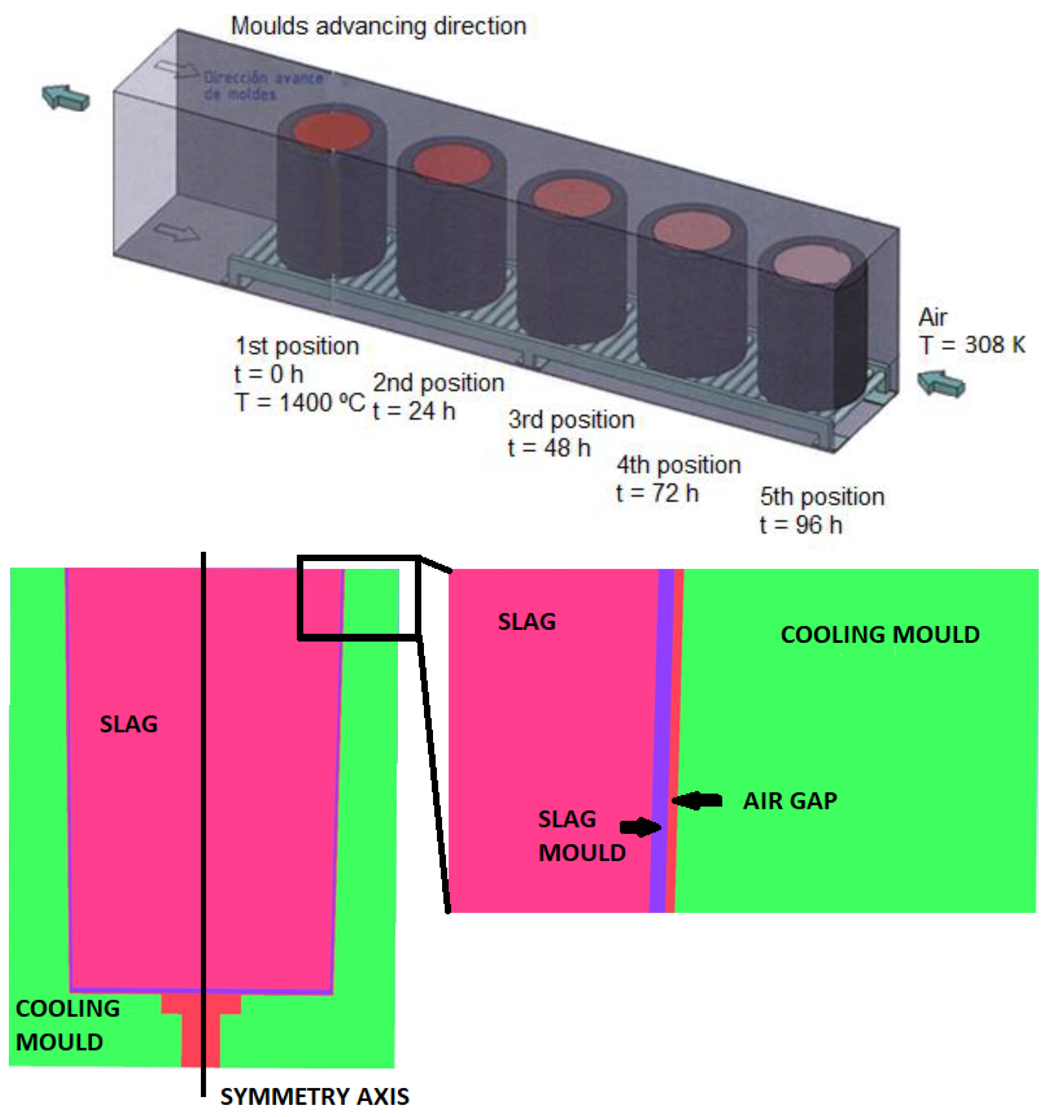
2.1. Description of the Process

The system under analysis is presented in Figure 1, where the operating procedure is the following:
  • The slag mould is filled up in the top part of the cooling tunnel (above drum position 1). After the slag mould is filled, it is located at position 1 inside the cooling tunnel, where air is flowing through in the opposite direction to the drums advancing direction.
  • After 24 h, drum 1 advances to location 2. A new drum is located at position 1 from the filling position.
  • Every 24 h, the drum advances to locations 3, 4 and 5, while it is being cooled down by means of the external air flow.
  • After 5 days the solid slag is taken out and the cooling mould is used again for the same process.
The objective of the cooling process is to achieve a slag maximum temperature below 323 K after 5 days, while minimizing the air flow rate needed and maintaining the air flow outlet temperature below 328 K.

2.2. Modelling Methodology and Assumptions

The information required for the modeling and simulation of the cooling process is related to the physical properties of the materials and to the operating conditions of the system. The geometry of the drums must also be carefully modeled. The following sections present all the data, modelling methods and model assumptions for the development of this work.

2.2.1. Geometry Modelling and Drum Dimensions

Figure 1 (top) shows the cooling system, where the drums are placed within an 8 m long walled parallelepiped, with air inlet and outlet at the sides as marked at the top of Figure 1. The cross-section area for the air inlet (see Figure 1) is 1.192 m (width) × 1.2 m (height).
Figure 1 (bottom) shows the vertical slice of the geometry of the drums to be cooled, where the cooling mould external diameter is 0.8 m. The main geometrical dimensions are listed in Table 1.
Both geometries have been modelled for the objectives of this study (i.e., the 3D air flow around the drums as depicted in Figure 1 (top), and separately the 2D axisymmetric interior of the drum as depicted in Figure 1 (bottom)). This is described in Section 2.2.4.

2.2.2. Slag and Mould Physical Properties

The slag physical properties are listed in Table 2. A slag assuming the physical properties of steel are considered for the cooling analysis. In a further sensitivity analysis (Section 3.5) a slag with the properties of glass is being considered in order to analyse the influence of the slag type.
The cooling mould material is spheroidal graphite cast iron with the following physical properties [32]:
  • Thermal conductivity: 36.2 W/m·K
  • Specific heat: 512 J/kg·K
  • Density: 7100 kg/m3
  • Thermal Expansion Coefficient: 12.5 μm/(m K)
An air gap thickness is included in the design (Figure 2) in order to account for the dilatation of the materials with the temperature change. The thickness of the air gap will therefore will vary along the cooling process. According to the maximum temperature expected for the slag mould (1673 K) and the Thermal Expansion Coefficient of the material, the maximum dilatation expected for the slag mould in radial direction is 9.0 mm, which would reduce the initial gap thickness accordingly.

2.2.3. Operating Conditions

The cooling air enters the system at 308 K according to the treatment plant operational data, and it is assumed to present a flat velocity profile. The air inlet is located as depicted in Figure 1 (top). At the initial time, the liquid slag and the slag mould temperatures are set to 1673 K for the first drum (Figure 1), as this is the temperature of the previous waste processing unit. The air gap and cooling mould temperatures are assumed to be at ambient temperature (323 K) at t = 0, at the time when the slag mould is inserted into the cooling mould.

2.2.4. Modelling Methodology

ANSYS-FLUENT [33] software was used for the Computational Fluid Dynamics (CFD) simulations. ANSYS-FLUENT is based on the Finite Volume Method (FVM), where the discretized Navier-Stokes equations are iteratively solved at the cell centres. The equation for conservation of mass, or continuity equation, can be written as follows [33]:
ρ t + · ( ρ v ) = S m
where the source Sm represents the mass added to the continuous phase from a second phase (which is zero in our case).
The conservation of momentum in an inertial (non-accelerating) reference frame is described by [33]:
t ( ρ v ) + · ( ρ v v ) = p + · ( τ ¯ ) + ρ g + F
where p is the static pressure, τ is the stress tensor), and F represents external body forces (which are zero in our case, as well as the gravitational forces).
The energy equation for heat transfer modelling is solved in the following form:
t ( ρ E ) + · ( v ( ρ E + p ) ) = · ( k e f f T ) + S h
where keff is the effective conductivity (k + kt, where kt is the turbulent thermal conductivity, defined according to the turbulence model being used). The first term on the right-hand side represent energy transfer due to conduction, and Sh represents volumetric heat sources (which are not of applicability in the current case).
In the solid regions within the drums, the energy transport equation for heat conduction used by ANSYS-FLUENT has the following form:
t ( ρ h ) = · ( k T ) + S h
where ρ is the density and h the sensible enthalpy.
The realizable k-epsilon model in ANSYS-FLUENT was used for turbulence modelling, with non-equilibrium wall functions [33].
The pressure-based solver was used for the simulations, with second order spatial discretization schemes for the momentum and energy equations, and the SIMPLE scheme was used for the pressure-velocity coupling [33]. An under-relaxation factor of 1.0 was used for the energy equation in order to ensure convergence. The convergence criteria were set to 1.0 × 10⁻³ (absolute) for all equations, except for the energy equation where 1.0 × 10⁻⁶ was used.
The heat transfer transient analysis of the entire system is complex in terms of CFD computing time, given the different scales in space and time and the consequent spatial and time discretization requirements. As an indication, the cooling air flow advection time is roughly 1 s, in comparison with the 5 days (4.3 × 10⁴ s) operating time of the system. A decoupled approach was therefore developed in order to enable the transient cooling analysis of the system. In order to carry out this, two different sub-systems are analysed:
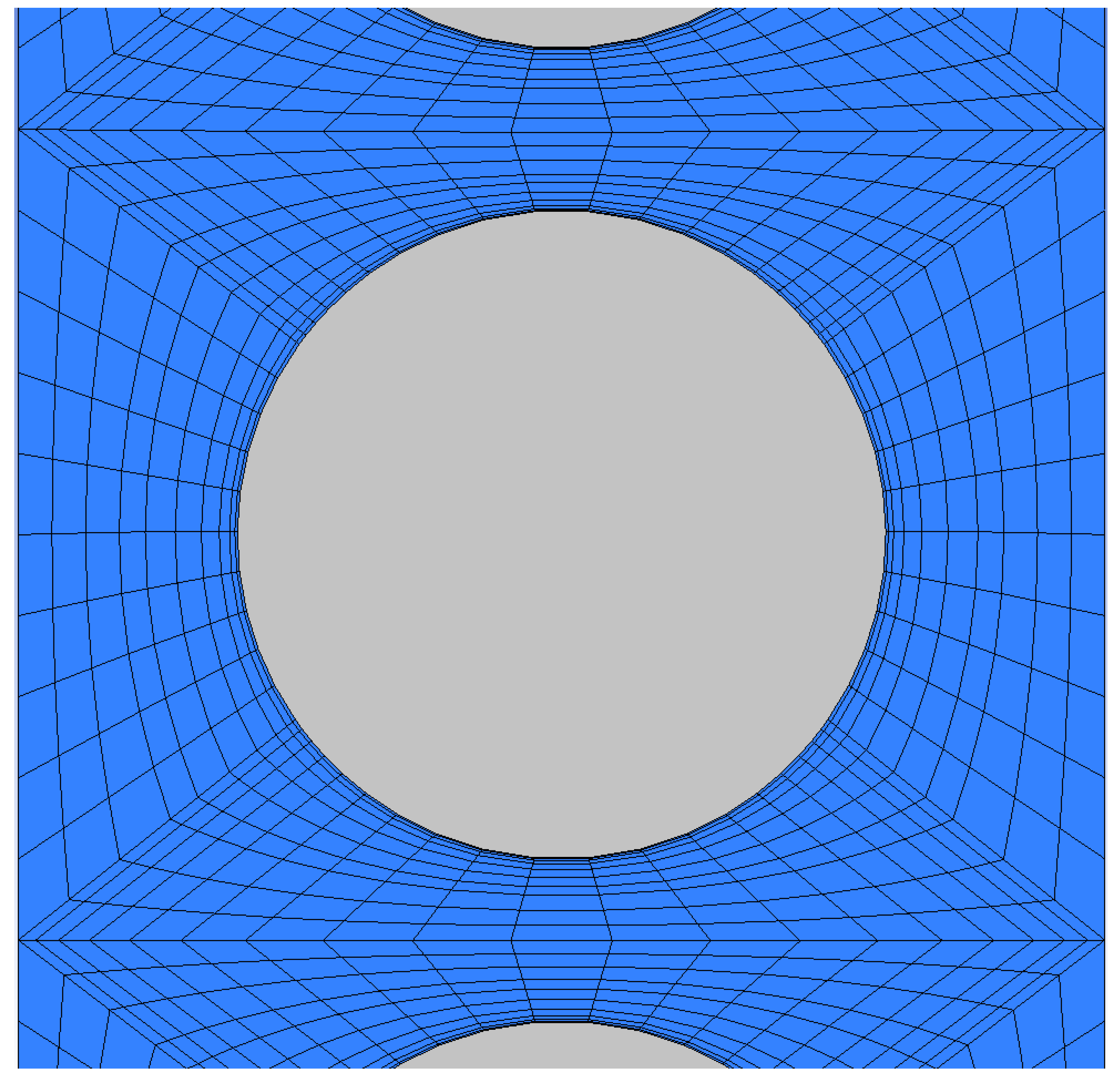
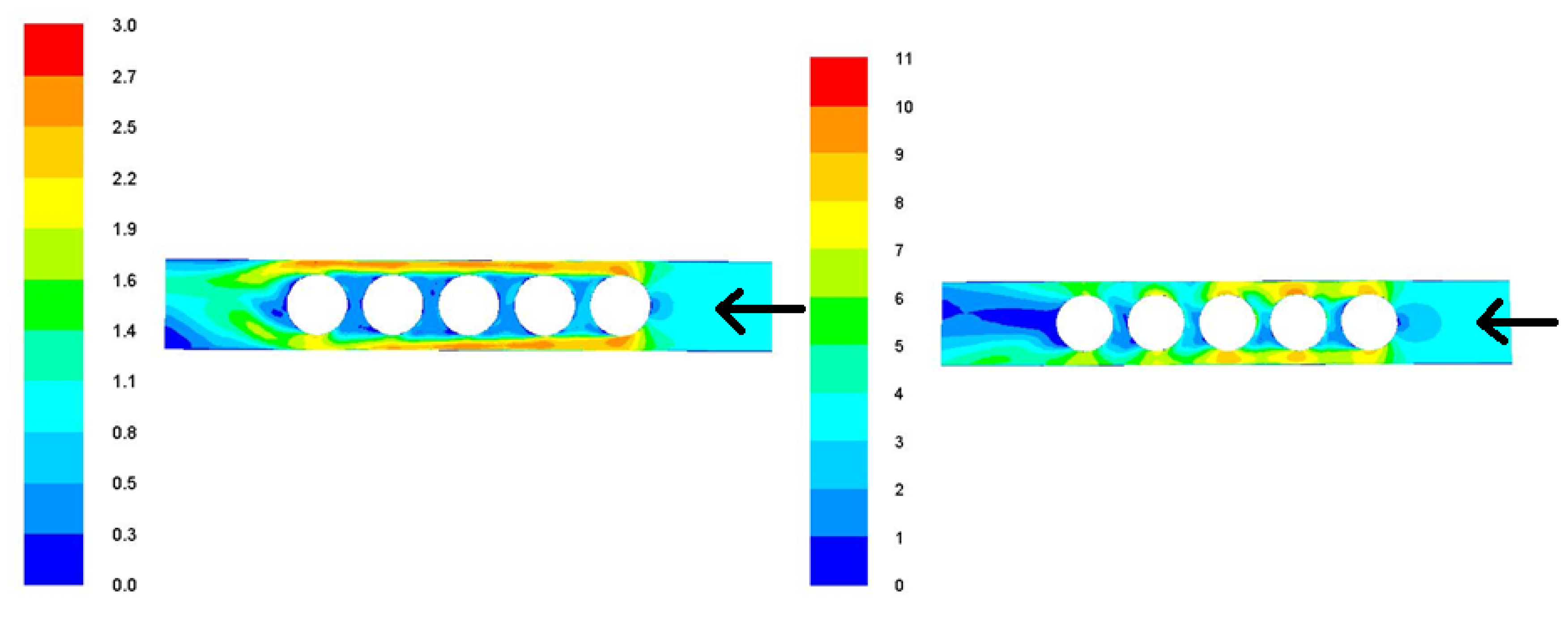
  • First, the external 3D air flow forced convection is solved around the five drums for a set of different air flow rates. Given the turbulent nature of the flow, the Realizable k-epsilon model in ANSYS-FLUENT was used for turbulence modelling, with non-equilibrium wall functions [33]. Simulations are carried out in steady-state. The drum external wall heat transfer coefficient is obtained as a result of the simulations, for each of the five drums in the row.
  • Second, the heat transfer within the different drum elements is resolved separately. 2D axisymmetric simulations are carried out given the symmetry nature of the cylindrical drums (axis is depicted in Figure 1 (bottom)). The transient cooling heat transfer process is resolved, using a constant initial temperature at t = 0 s (1673 K for slag and slag mould, and 323 K for the other drum elements). The boundary condition at the external wall of each drum is the heat transfer coefficient calculated from the previous 3D simulation of the air flow around the drums.
  • The coupling interface between both simulations is therefore the external wall of the drums.
The air flow around the drums as depicted in Figure 1 (top) was analysed by means of 3D CFD simulations, ensuring y+ values in the range of 1–10 to correctly capture the turbulent and thermal boundary layer [33]. A complete set of simulations were carried out for different air flow velocities and drum external wall temperatures, with the aim to calculate the heat transfer coefficient. As the main features of the air flow field do not depend on the drums cooling, all simulations were carried out in steady-state.
However, the cooling process in the drums is obviously a transient process. This process is governed by heat conduction within the drum elements, and forced heat convection to reject heat into the external air flow. In order to simulate this, 2D axisymmetric simulations of the drum geometry were carried out in transient mode, setting the external heat transfer coefficient to the values obtained in the previous step. The phase change of the slag has been accounted for by defining a specific heat capacity (Cp) as a function of temperature, where the Cp value at the solidification temperature has been increased so that the integral of the Cp peak vs temperature is equal to the phase change enthalpy.
As the melting point of the slag is exactly the slag temperature at t = 0 s, the latent heat of the slag was accounted for in the simulations simply by setting a constant slag temperature until the heat transferred from the slag to the slag mould reached exactly the value of the latent heat times the mass of the slag.

2.2.5. Model Assumptions and Boundary Conditions

The assumptions used for the simulation are the following:
  • Equal slag properties for solid and liquid phase (detailed in Table 2), as nuclear waste slag properties are not known. A sensitivity analysis for the slag properties is carried out in Section 3.5 in order to evaluate the effects of the variation of the slag properties.
  • Slag mould properties equal to the slag properties (as nuclear waste slag properties are not known). A sensitivity analysis for the slag properties is carried out in Section 3.5.
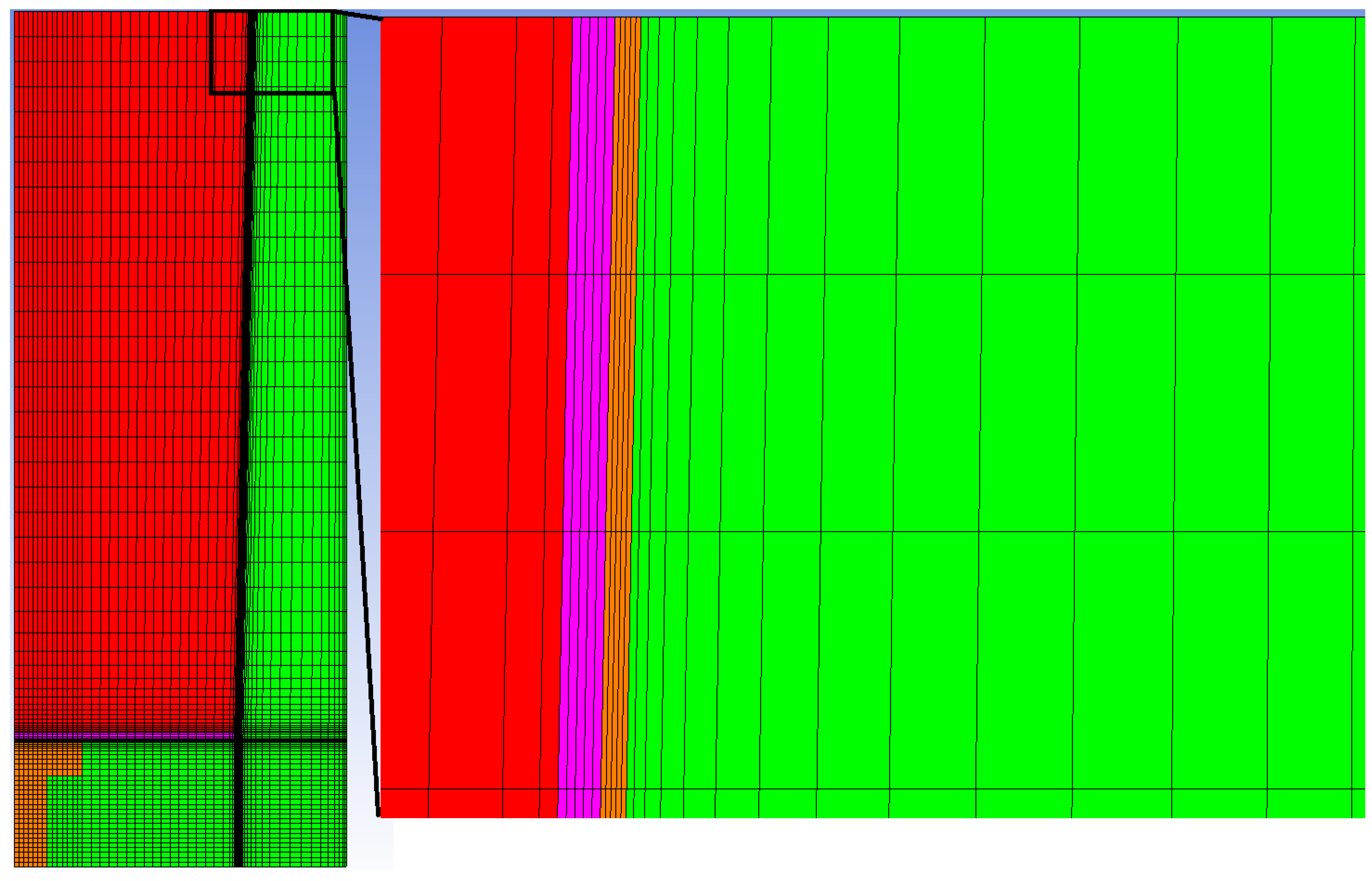
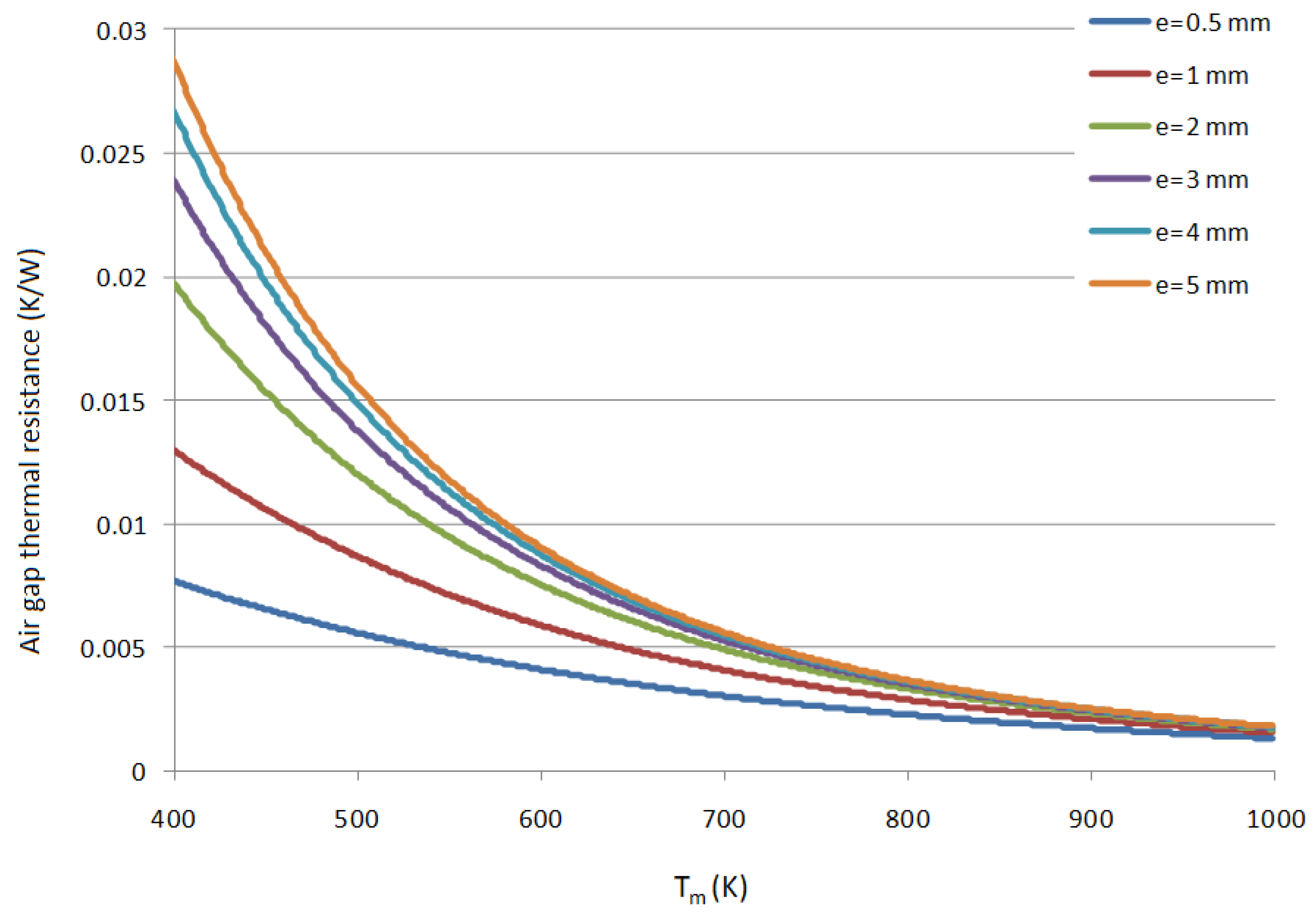
  • The air conductivity in the air gap (0.5–5 mm thickness depending on the dilatation state) is corrected in the CFD simulations in order to take into account the radiation heat transfer between slag mould and cooling mould. This assumption is described and justified in Section 3.1.
  • Constant air velocity at the inlet section (flat velocity profile at the inlet considered, as the real velocity profile from the blower upwind is not known).
  • External heat transfer coefficient is dependent on drum position (see Figure 1), as turbulence and flow field around drums will differ for each drum. However, it is assumed to be constant for the top and side drum surfaces. This assumption is based on the preliminary results obtained for the simulations (29.18 W/m2K at the top surface and 29.24 W/m2K at the side, for the third drum at 2 m/s air velocity).
  • Adiabatic bottom drum surface, as the heat flow through the bottom surface will be negligible in comparison with the side and top surfaces, given the very low air circulation under the drums as a result of the system configuration (Figure 1, with drums laying on the rolling floor).
  • Gravity is not included in the simulations. The drum external heat transfer is a process governed by air flow forced convection, and the internal cooling is dominated by heat conduction within solids. Gravity forces can be therefore neglected.
  • Drum-drum radiation heat transfer and drum-wall radiation heat transfer has been neglected in the simulations, as preliminary estimations show that radiation effects are negligible (drum-drum view factor is 0.15). Simulation results will be therefore minimally affected by radiation heat transfer, and not including it in the model will provide conservative results.
  • The drum is perfectly cylindrical with a central rotation axis. Therefore, in order to allow for shorter computation times, a 2D axisymmetrical segment of 3 degrees has been resolved instead of the full 360-degree geometry (axis is depicted in Figure 1b). This allows for a mesh with less elements than in a 3D geometry, and it fully represents the real drum geometry.
  • Time step size = 100 s. As the total cooling time is 24 h, 100 s time step size means 864 time steps.
The boundary conditions defined are the following:
For the 3D external air flow around the drums, a set of simulations with different air inlet velocity values is defined (1 m/s to 5 m/s). The air outlet is defined to be at atmospheric pressure. The side walls, top and bottom are considered as adiabatic. For each air inlet velocity condition, the drums external wall boundary condition is defined with a fixed temperature, where a set of different simulations with different wall temperatures have been carried out (from 373 K to 1473 K). The objective of this is to verify the dependence of the wall heat transfer coefficient on the drum external wall temperature, which will depend on the time along the cooling process. As mentioned in the model assumptions section, the bottom wall of the drums is considered adiabatic.
For the 2D internal heat conduction within the drums, the only boundary conditions required are the side, top, and bottom. As mentioned in the model assumptions section, the bottom wall of the drums is considered adiabatic. The side and top walls boundary conditions are defined with the heat transfer coefficient obtained from the previous 3D external flow simulation, and the ambient temperature of 308 K (which is the inlet air temperature).

3. Results

In this section the following results are provided and discussed:
  • Analysis of the thermal resistance of the air gap between slag mould and cooling mould, in order to assess the relative importance of heat radiation in comparison to conduction.
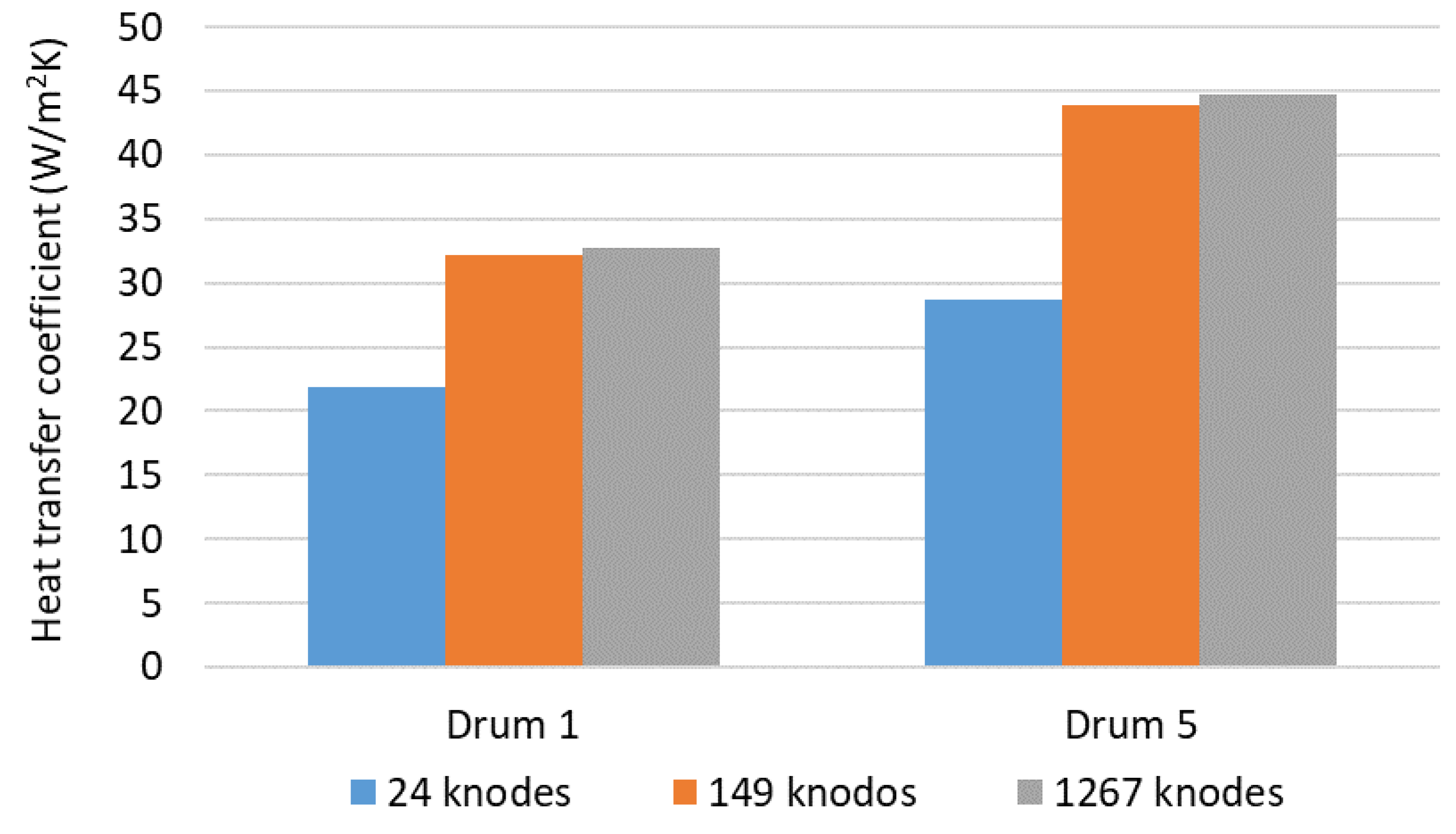
  • Analysis of the external convective heat transfer coefficient of the drum wall-air interface by means of 3D CFD simulations.
  • Determination of the temperature profiles (in space and time) in the drums by means of 2D axisymmetric CFD simulation.
  • Determination of the outlet air temperature.
  • Sensitivity analysis for different slag properties.

3.1. Analysis of the Thermal Resistance between Slag Mould and Cooling Mould

The air gap formed in the gap between slag mould and cooling mould introduces a resistance to heat transfer between the slag and the cooling air outside the drum. This thermal resistance must be evaluated in order to assess its importance in the overall heat transfer process. The thermal resistance is a function of conductive exchange between the external surface of slag mould and interior surface of cooling mould through the air between the two, and radiation heat exchange between two surfaces due to temperature difference. Because the thickness is less than 5 mm, the Nusselt number is assumed to be unity, so there will not be a convective heat transfer between walls and air.
The thermal resistance is calculated by the following expression [34,35]:
R a c = 1 2 π k a i r L s ln ( r e , s m + thickness r e , s m ) + 4   ε   σ   T m 3 A s
where: Ls is the length of slag, As is the heat transfer area of slag, thickness is the thickness of air gap and Tm is the average temperature of the air gap and is defined by:
T m = T e , s m + T i , c m 2
The temperature of the walls will determine the air temperature in the gap (also, its thermal conductivity) and radiant heat flow between them.
Figure 2 shows the thermal resistance value based on the average temperature of the walls for different thickness considered in a sensitivity analysis to cover the possible dilatation states: 0.5, 1, 2, 3, 4 and 5 mm. It is shown that the resistance decreases at higher temperatures due to the effect of radiant heat transfer between surfaces. For any given average temperature, when the thickness of the air gap increases the thermal resistance also increases. For average temperatures above 600 K, the thermal resistance of the air gap is significantly less than the convective thermal resistance at external cooling mould surface (which is about 0.01 K/W). Therefore, the external forced convection is in general the controlling heat transfer resistance in the overall cooling process. Nevertheless, the thermal conductivity of the air within the gap has been corrected in the simulations, in order to account for the increase of the heat transfer due to surface radiation between mould surfaces.

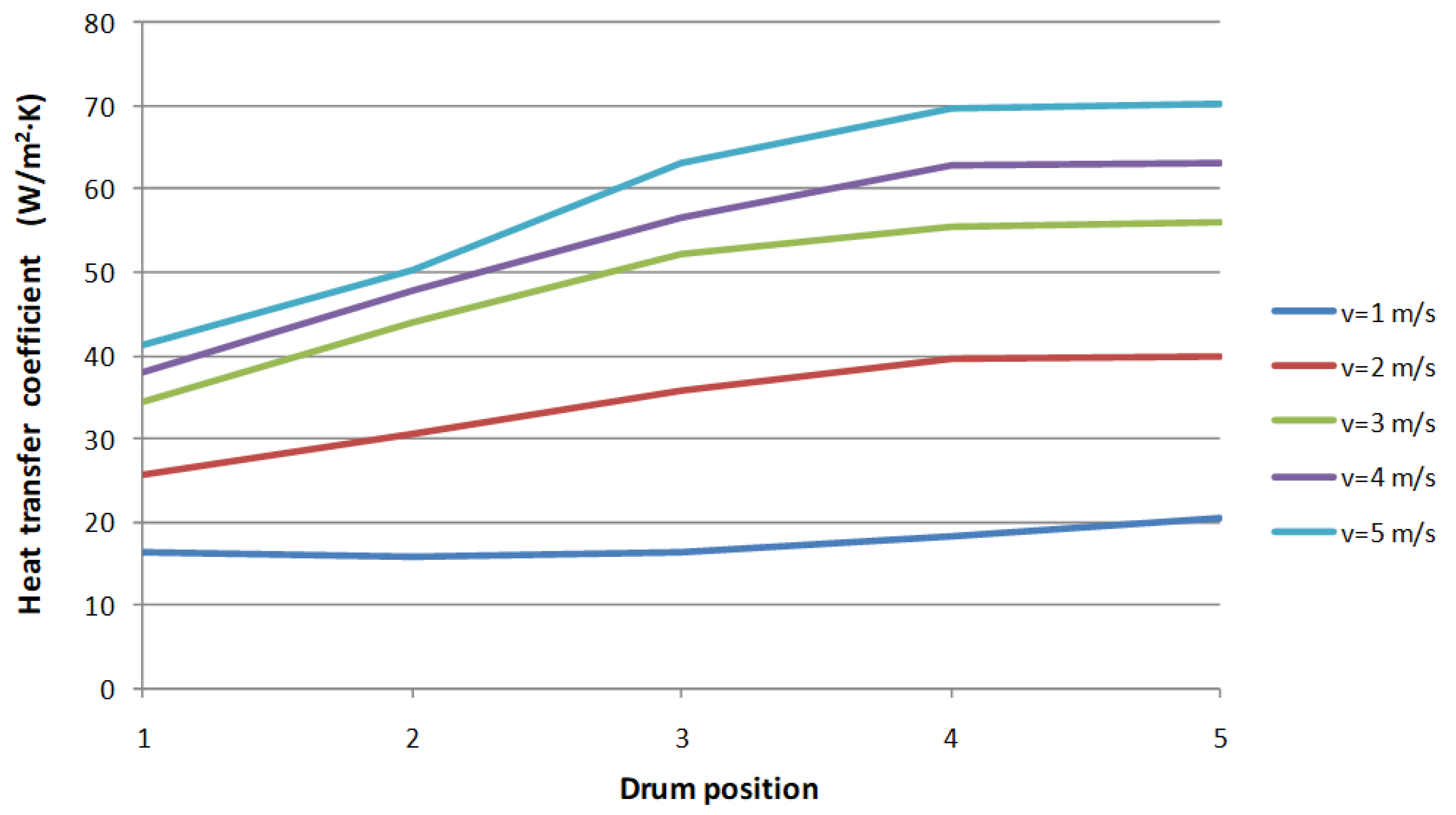
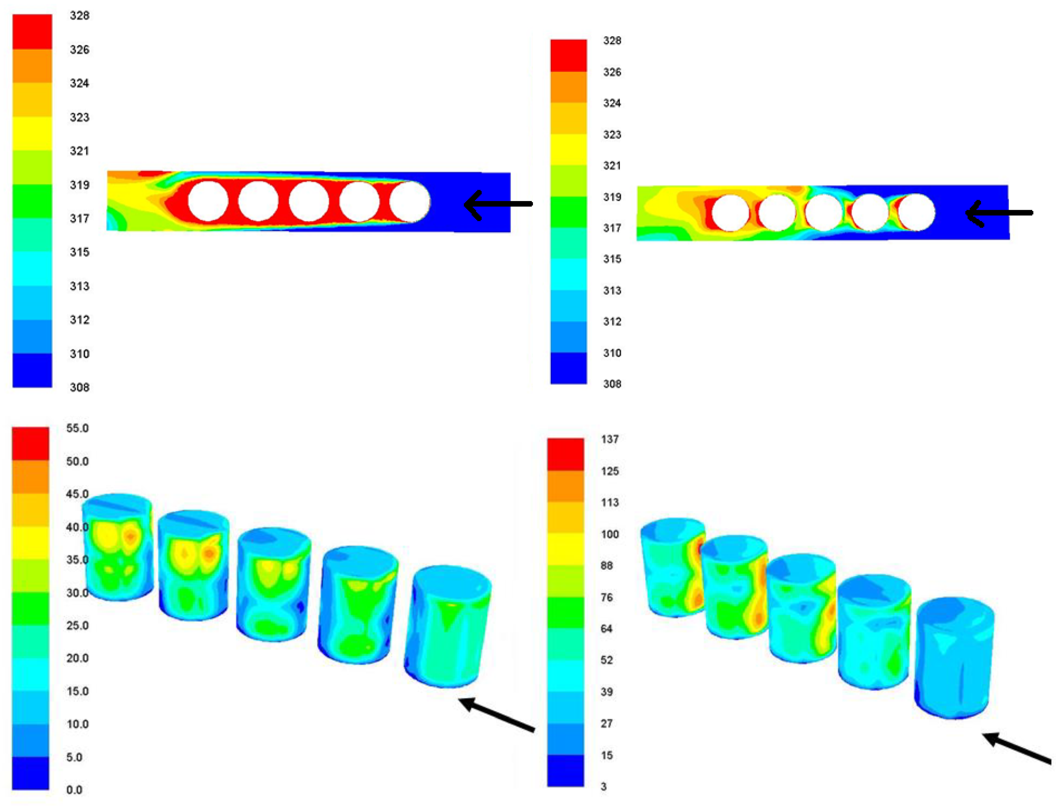
3.2. Analysis of the Mould/Air External Forced Convection

The heat released by the slag through the different elements of the complete drum must be transferred to the air flow by means of an external forced convection mechanism. The set of five cylindrical drums constitutes a typical heat transfer analysis problem similar to cross flow through an array of tubes [34].
Determining the heat transfer coefficient hext is essential for the analysis of the overall problem. This coefficient is depending on the flow velocity and properties, as well as on the system geometry. Although some empirical correlations exist for the calculation of hext in such system, they provide a unique average value for the complete set of drums, with relatively significant errors. Therefore, hext were determined by means of detailed 3D Computational Fluid Dynamics (CFD) simulations of the heat transfer and air flow around the drums. Results of hext for each drum can be obtained from the CFD simulations. Results were obtained for a set of different drum external temperatures and air velocities.
A mesh dependency was carried out in order to ensure that a correct mesh density and refinement is used. Three different meshes were generated, each of them doubling the number of elements in each coordinate x, y, z with respect to the previous one. Thus, each mesh is approximately a factor 8 finer than the previous one. In all cases the mesh was refined towards the drums wall. The resulting meshes (a coarse mesh having 24,500 nodes, a medium mesh with 149,500 nodes and a fine mesh with 1,267,500 elements) were simulated for the case with 3 m/s air velocity and 473 K drum wall temperature. The drums wall heat transfer coefficient for drum positions 1 and 5 (the most extreme ones) was reported as the control variable for the mesh dependency analysis. Results are presented in the Figure A1. It is observed that hext results for the coarse mesh are significantly low, but however the values obtained for the medium and fine meshes are very similar presenting differences of about 1%. As a conclusion of the study, the medium mesh was used for all the simulations reported below, as it presents accurate results without excessive computational cost.
Thus, the 3D mesh with 149,500 hexahedral elements and mesh refinement towards the drum walls was used (depicted in Figure A2). The cell elements aspect ratio was maintained below 100, skewness above 0.35, and face angles over 30 degrees. The average cell size ∆x was 0.04 m, with mesh refinement towards the drum wall where the first node is located at 2.0 × 10⁻⁴ m from the wall, in order to achieve the required y+ values for the resolution of the turbulent boundary layer. The Realizable k-epsilon model in ANSYS-FLUENT was defined for turbulence modelling, with non-equilibrium wall functions [33].
The CFD simulations were performed for air flow velocities in the range 1 m/s–5 m/s, corresponding to an air flow rate between 5.120 and 25.750 m3/h. Re number (based on the drum diameter and the maximum velocity) is ranging from 1.9 × 10⁵–9.6 × 10⁵, and therefore the flow is fully turbulent.
Figure 3 show details of the 3D air flow resolution around the drums for air velocity 1 m/s and 3 m/s, where the air flow direction is indicated by an arrow. The velocity profiles are clearly observed in Figure 3 (top), where the local flow acceleration on the drum sides caused by the reduction in the cross-section area is more significant for 3 m/s. Behind the drums a low velocity area is generated as is typical for the flow over cylinders. The pressure drop across the system as resulted from the simulations is 8 Pa for 1 m/s and 45 Pa for 3 m/s.
The air local temperature distribution is presented in Figure 3 (middle), where the progressive heating is clearly observed. It must be considered that in this simulation the drums external temperatures were defined at 373 K. The present analysis is aimed at the determination of the external heat transfer coefficients, where the influence of the drum external temperature is not significant in the temperature range expected. This has been demonstrated by calculating hext at different wall drum temperatures in the range 323–1273 K.
Finally, Figure 3 (bottom) shows the local heat transfer coefficients over the drum walls, which obviously present larger values for 3 m/s. In order to calculate a unique heat transfer coefficient value (for each drum position) from the local distribution shown in Figure 4, an area-average value was determined for each drum. This value will be later applied in the subsequent 2D simulations at the drum wall in order to calculate the transient cooling process of the drums. This assumption will allow for the 2D simulation of the cooling process of each drum. In addition, it must be considered that despite the fact that the heat transfer coefficient is not constant over the cooling mould external wall (Figure 4) the relatively high thermal conductivity of the cooling mould material will uniformize the temperature field, and heat will be therefore more uniformly transferred from the slag towards the external wall.
The resulting heat transfer coefficient for each drum is reported in Table 3, where di is the drum position number according to Figure 1.
The results show that the heat transfer coefficient increases for higher air velocities as expected. It is also observed that hext increases as the drum position increases (until position 3–5), which is a well-known phenomenon caused by the progressive increase in the turbulence levels as the flow passes along the drums [34,35]. hext then reaches a constant level after 3–5 drums.
It is important to note that as the heat transfer coefficient is not dependent on the material or internal configuration of the drum, it has the same values for the different materials tested (steel, glass) and for the different air gap thicknesses, and will be therefore used for all the simulations hereafter. Simulations were also carried out for different drum wall temperatures, and it was verified that wall temperature is having a very small effect in the heat transfer coefficient, as could be also predicted by analyzing the heat transfer correlations commonly used for flow around bank of tubes. As an example, Zhukauskas correlation [34,35] uses constant fluid properties at the inlet temperature, and then corrects this by the factor (Pr/Prwall)1/4, which for the worst case analysed (308 K inlet air temperature and 1473 K wall temperature) is 0.9964, therefore influencing the Nusselt number by less than 1%. For the sake of completeness, the results for all simulations (average heat transfer coefficient for each drum position, for the matrix of air flow velocities and drum wall temperatures) are included as supplementary material (Table S1).

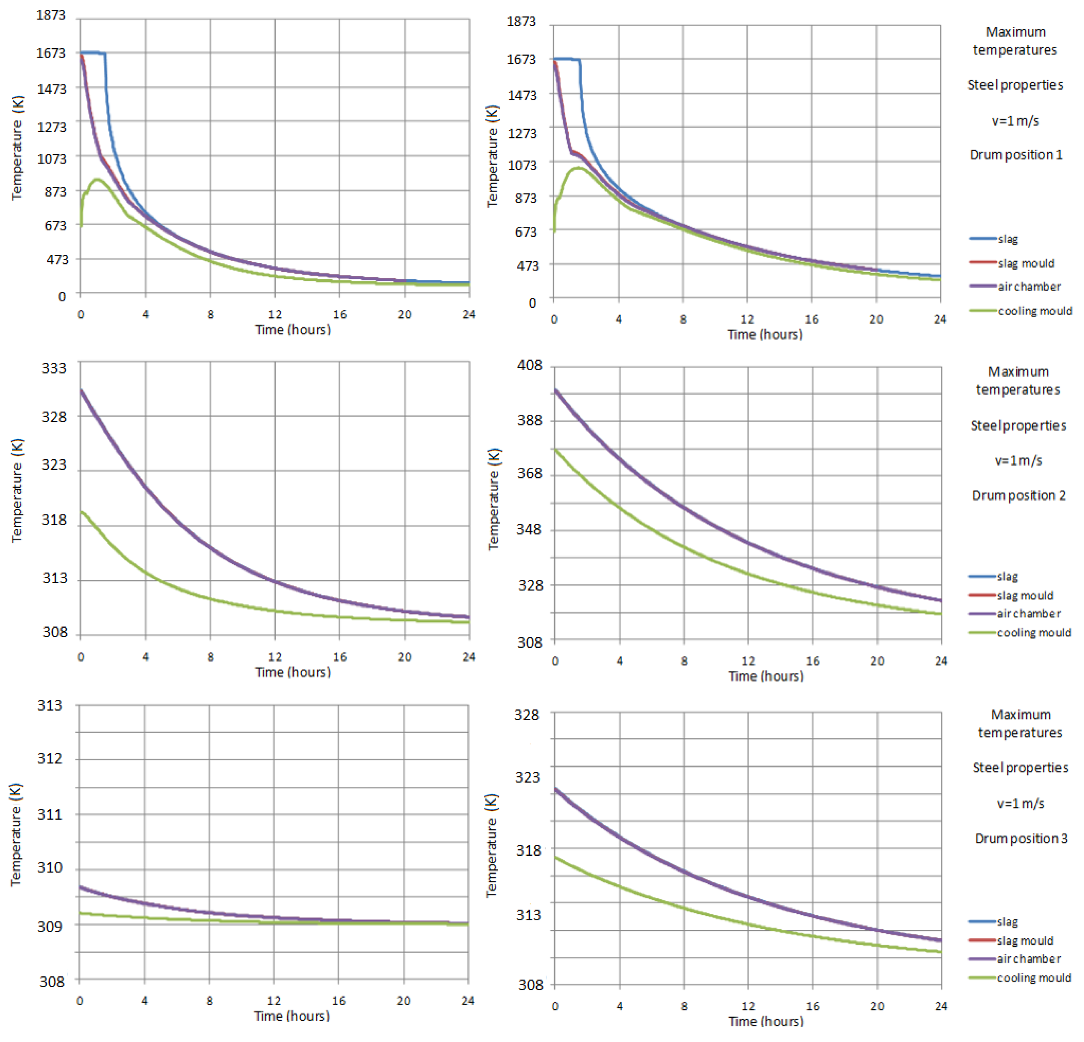
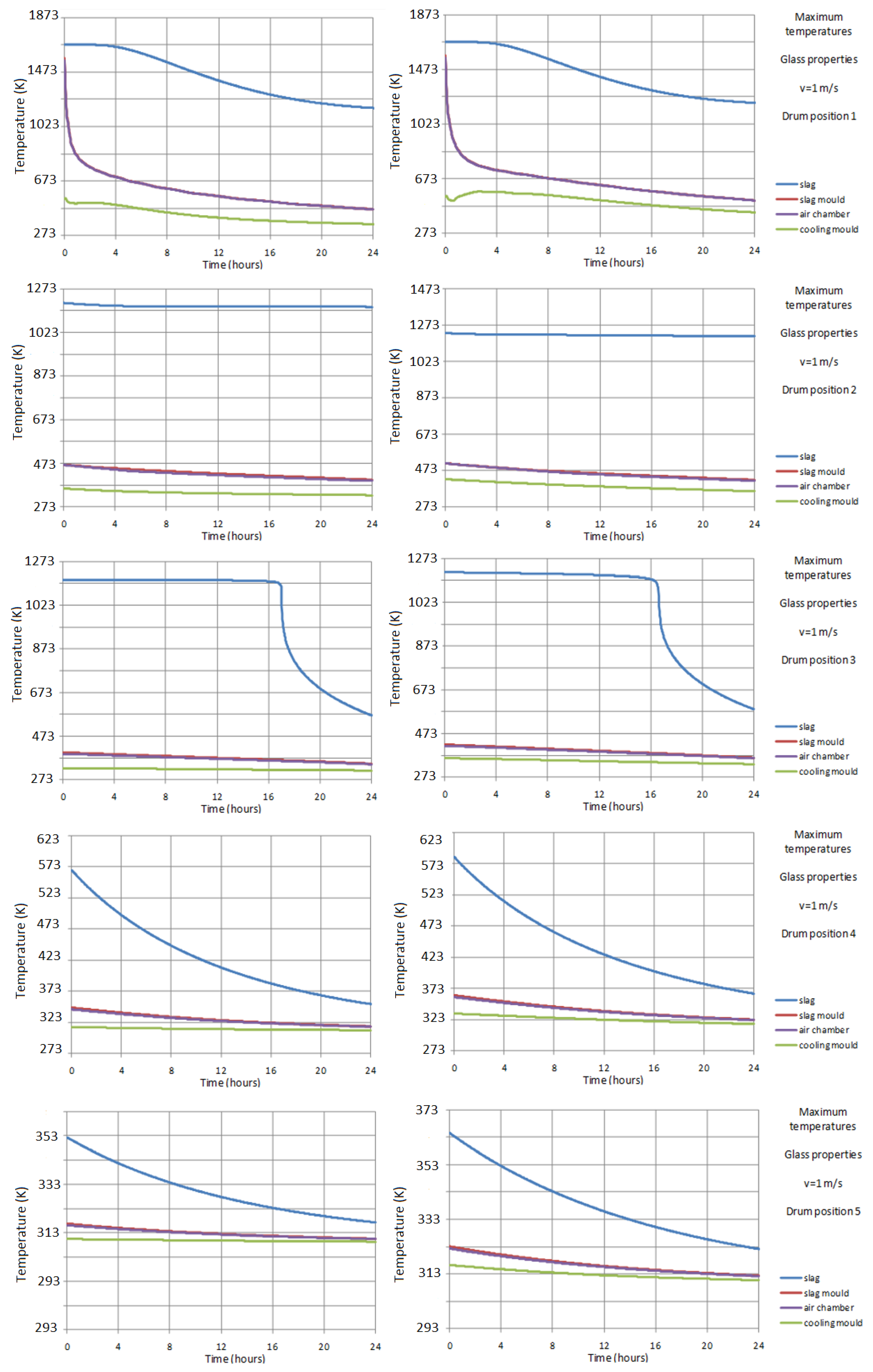
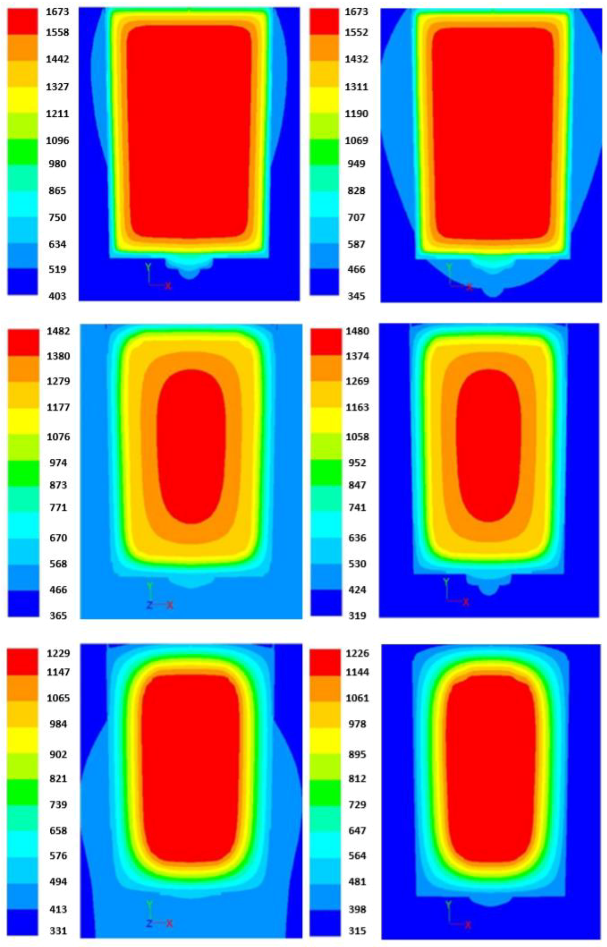
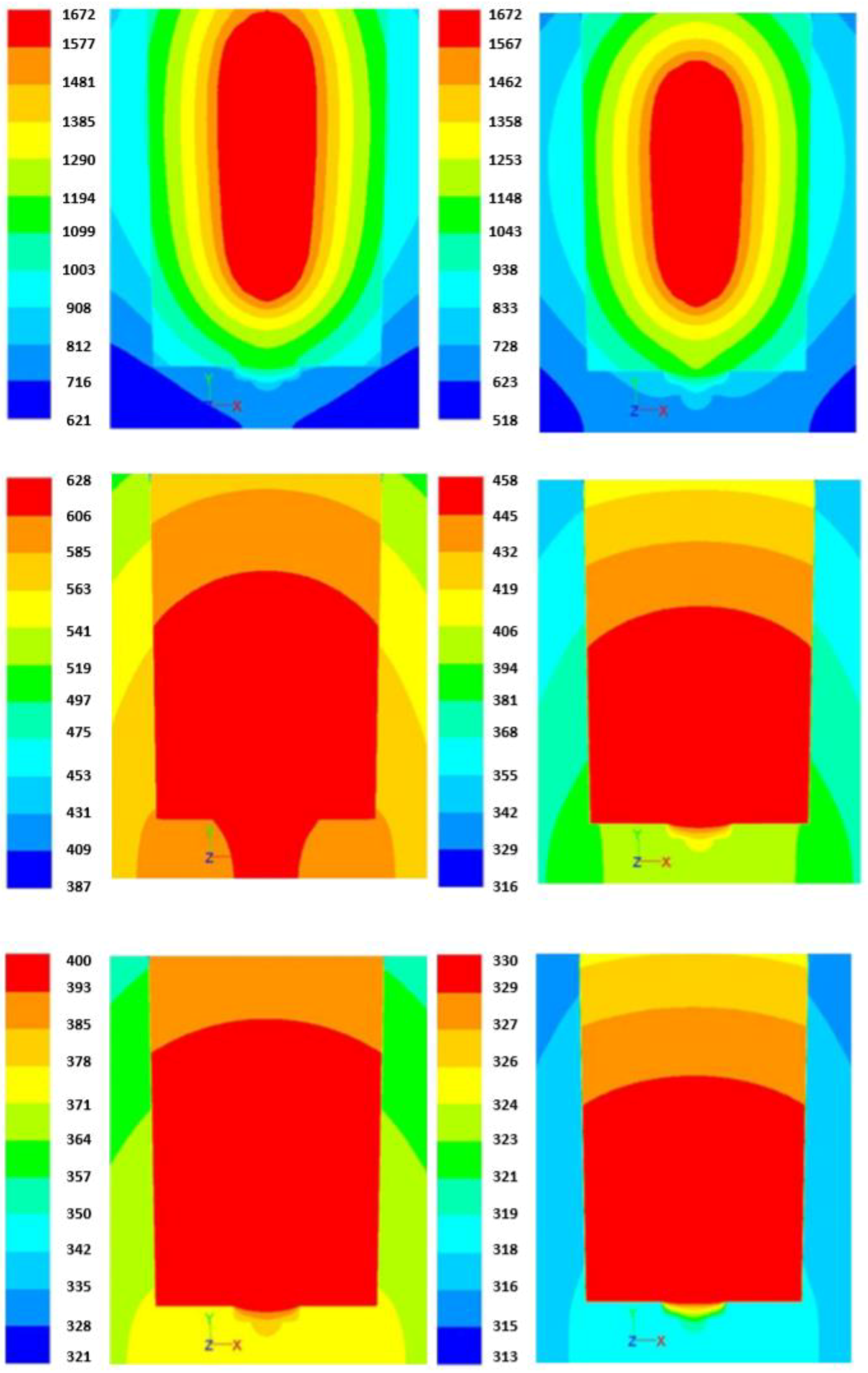
3.3. Temperature Distribution in Drums

The time evolution of the temperature of the elements within a drum (slag, slag mould, air gap and cooling mould) during the cooling process for each drum position is determined in this section by means of 2D CFD simulations carried out with ANSYS-FLUENT.
A 2D hexahedral mesh with 4775 elements was used (depicted in Figure A4). Although 3 mesh elements are typically enough for resolving heat conduction in thin elements [33], 5 elements were used in the slag mould and air gap thickness in the simulations, in order to ensure the accuracy of the results. Thus, a cell size of Δx < 0.001 m was used to resolve the heat conduction in the critical elements of the drums. Mesh refinement was also used around both slag mould and air gap as depicted in Figure A4. Second order discretization scheme was used.
Figure 4 (left) presents the time evolution of the maximum temperature for each element at each drum position (each position lasting 24 h, and thus completing the 5 days of cooling when all five positions are considered). Results in Figure 4 correspond to the slag with steel properties and an external air velocity of 3 m/s.
Drum 4 and drum 5 present an almost constant temperature of 309 K. As evidenced in Figure 4 (left), the largest cooling within the drum occurs when it is located in position 1. Also, the maximum temperature of the slag (located at the centre of the drum) drops from 1673 K to 330 K in 24 h. The final accepted conditions for slag (maximum temperature less than 323 K) are nearly reached when the drum is still in position 1. It is also observed in Figure 4 that the slag solidification time is less than 2 h.
The maximum temperature of the cooling mould is 934 K, and it is reached one hour after the start of the cooling process. During this time, cooling mould temperature increases due to the heat flux received from the slag through the air gap, which is higher than the heat flux dissipated to the external air by external forced convection in this particular case. It is important to ensure that the maximum temperature reached is below the melting point of the mould material in order to preserve it, which is fulfilled in this case.
When an external air velocity of 1 m/s is considered, the corresponding cooling curves are presented in Figure 4 (right). Conclusions are similar than in the previous case, where again the largest cooling process within the drum occurs when it is located in position 1. However, the cooling process is obviously slower, with a maximum temperature of the slag dropping from 1673 K to 399 K in 24 h. The final conditions for the slag (maximum temperature less than 323 K) are reached after 48 h. The maximum temperature of the cooling mould is 1036 K for this conditions, and it is reached 1.5 h later from start time of the cooling process.
The spatial temperature distributions for both cases (air velocity 1 m/s and 3 m/s) at different times during the cooling process are presented in Figure 5. Temperature profiles at a transversal plane for time = 1 h, 10 h and 24 h are presented. Temperature profiles are qualitatively similar at every time for both velocities, but temperature values are less for air velocity = 3 m/s given the higher convection heat transfer coefficient. After 1 h since the cooling process start, heat from the slag is quickly being transferred to the cooling mould and external air, while a relatively large core of liquid slag remains in the centre of the slag mould. It can be observed that a lesser temperature (100 K less) is obtained in the cooling mould for the air velocity = 3 m/s, given the higher convection heat transfer coefficient. After 10 h, the slag has completely solidified and the cooling process is continuously evacuated through the cooling mould, which becomes much cooler than at 1 h, especially for air velocity = 3 m/s. After 24 h, the slag temperature has drop to values close to 323 K for air velocity = 3 m/s, and 403 K for air velocity = 1 m/s.
Table 4 shows maximum temperature of drums elements (slag, slag mould and cooling mould) for each cooling air velocity considered. When cooling air velocity increases, maximum cooling mould temperature decreases due to the higher heat transfer between cooling air and cooling mould at every time.

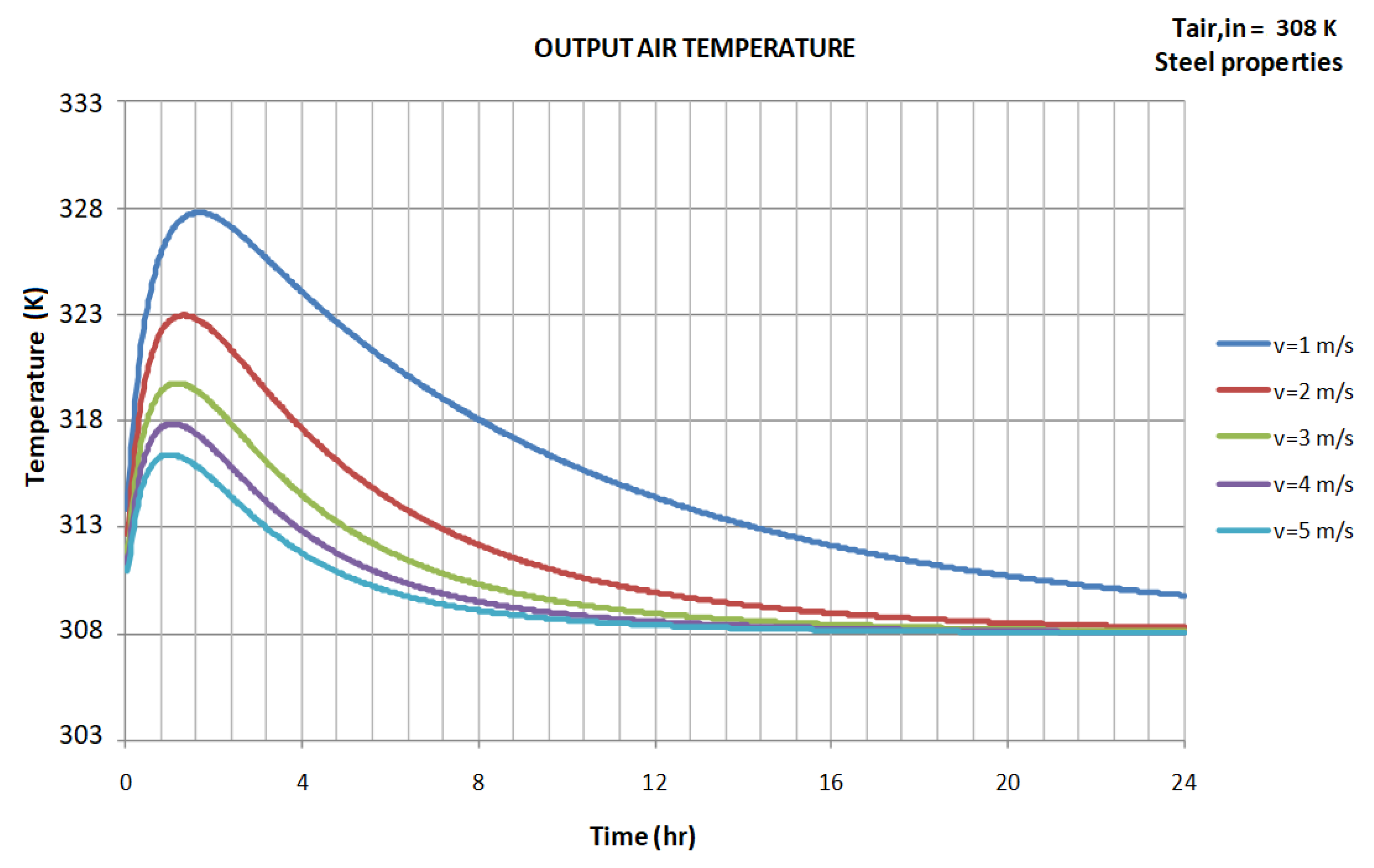
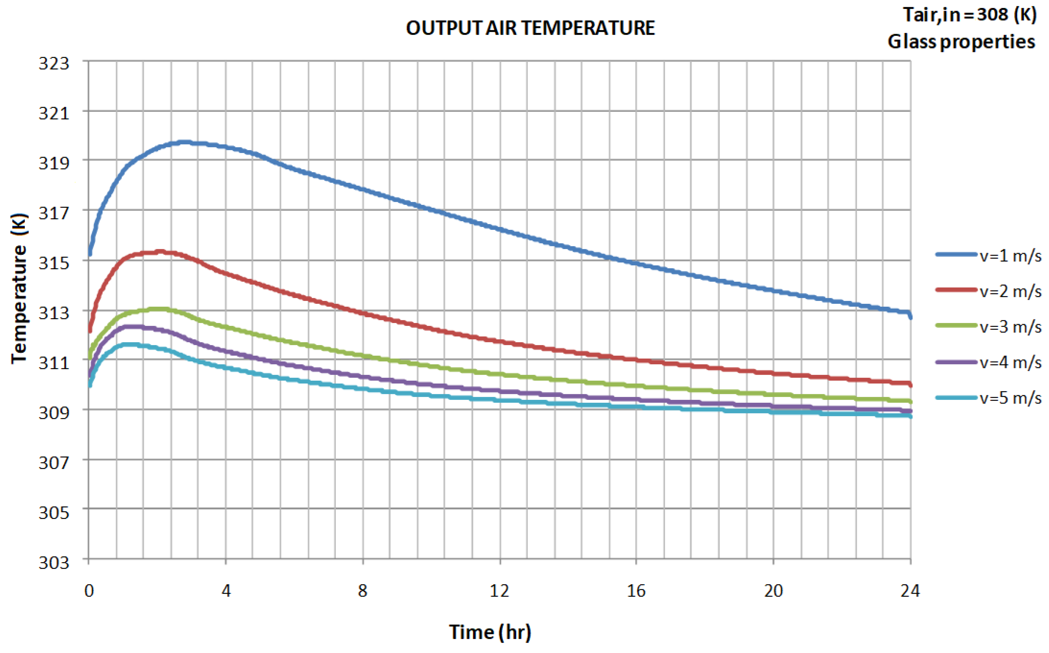
3.4. Air Outlet Temperature

The air outlet temperature at every time is calculated from its inlet temperature, flow rate, and heat flow evacuated by the drums, according to an energy balance:
T a i r , o u t = T a i r , i n + i = 1 i = 5 Q ˙ i m ˙   C p a i r
The heat fluxes are calculated by means of a transient simulation of the complete drum cooling process, using the simulation software ANSYS-FLUENT for each air flow condition. The process has been simulated for each of the slag materials considered (steel and glass) for air velocities in the range 1–5 m/s, during 24 h of system operation where most of the cooling process takes place as shown in the previous section. Figure 6 shows the air flow temperature evolution at the outlet, considering the slag as steel.
It can be observed that the maximum air temperatures at the outlet are reached during the first hours of operation after a new mould is located in position 1. This is caused by the significant heat flow dissipation during the initial hours (the maximum temperatures are reached between 1–1.3 h). The maximum cooling air temperature at this time for 1 m/s is 328 K.

3.5. Sensitivity Analysis

In this section a sensitivity analysis varying the slag physical properties is considered. Performing simulations considering the properties of glass for slag provides the following variations of maximum temperatures of the drum elements, in the five drums, during the first 24 h. Figure 7 (left) presents the time evolution of the maximum temperatures considering a cooling air velocity of 3 m/s, whereas Figure 7 (right) presents the time evolution of the maximum temperatures for an air velocity of 1 m/s.
When considering glass properties, the temperature of the elements in drum decreases significantly slower due to the lower slag conductivity, as heat conduction within the slag becomes the highest heat transfer resistance. It must be considered that Bi number is 0.3–0.5 (depending on the drum position) when steel properties are considered for the slag, but it rises to 25–40 when glass properties are considered.
For the first drum, 4 h after of the start point of process the slag core begins to decrease its temperature from 1673 K. During the first 24 h the slag core temperature decreases only from 1673 K to 1223 K. In drums 2 and 3 the solidification of slag occurs at a temperature of 1173 K. The solidification process takes approximately 41 h. The final slag accepted condition (maximum temperature below 323 K) is reached for drum 5 at 16 h (112 h total time).
For a cooling air velocity of 1 m/s the overall heat transfer process is slower, and for the first drum, 4 h after of the start point of process the slag center begins to decrease its temperature from 1673 K, reaching 1228 K after 24 h. In drums 2 and 3 the slag solidification occurring at a temperature of 1173 K takes approximately 42 h. The final accepted slag condition (maximum temperature below 323 K) is reached for drum 5 after 24 h (120 h total time, therefore at the limit of the system analysed).
It is observed that the temperature profile for the different air speeds does not present a pronounced peak as in the case of steel, due to the lower conductivity of the material that causes a heat transfer from drum more uniform over time. Again, the highest temperatures occur in the early hours of the day due to the high heat transfer in the first drum associated to high temperatures in external cooling mould surface. Table 5 shows the maximum temperature of the drums elements (slag, slag mould and cooling mould) for each cooling air velocity. When slag is simulated using glass properties, it is observed that the effect of cooling air velocity on the maximum elements temperature is neglected, due to the low conductivity of slag which becomes the heat transfer limiting rate.
Figure 8 show the temperature distributions at different times during the cooling process for the glass material and air velocity 1 m/s and 3 m/s. Local temperature distributions are presented for time = 1 h, 10 h and 24 h at a transversal plane. Temperature profiles are qualitatively similar at every time for both velocities, but temperature values are obviously less for air velocity = 3 m/s, given the higher convection heat transfer coefficient.
After 1 h from the start of the cooling process, heat from the slag is quickly being transferred to the cooling mould and external air, while a relatively large core of liquid slag remains in the centre of the slag mould. The fraction of liquid slag is much larger than the previous case where the slag is modeled with steel properties, given the much larger solidification enthalpy. It can also be observed that the cooling mould is 50 K cooler with air at 3 m/s than with air at 1 m/s. After 10 h, the slag is not yet solidified and a large liquid fraction remains, while the cooling process is continuously evacuated through the cooling mould. Again, the cooling mould is 50 K cooler with air at 3 m/s than with air at 1 m/s. After 24 h, the slag temperature is still over 1173 K and with a significant liquid fraction.
Considering glass properties, Figure 9 shows the time evolution of the outlet air temperature. For this material, air velocities between 2 and 5 m/s allow output air temperature to be under 318 K. However, for 1 m/s, air outlet temperature is above 318 K at 0.75–7.6 h. The maximum outlet air temperature for this velocity is 320 K.

4. Conclusions

In this work, the thermal and heat transfer characteristics of a radioactive waste processing unit have been investigated, with the objective of achieving a maximum accepted slag temperature of 323 K after 5 days of cooling. Computational Fluid Dynamics has been used for the simulations. Given the different time and length scales present in the system, the CFD simulations have been decoupled, solving separately the 3D steady-state flow around drums for obtaining the forced convection heat transfer coefficient, and the axisymmetric 2D transient heat transfer within the drum materials.
The system analysis has provided the following conclusions:
  • For all system variations analyzed, covering a range of air flow velocity 1–5 m/s and two different nuclear waste slag materials, the maximum temperature of slag is below 323 K at the end of five days operation, thus fulfilling the system requirements.
  • The maximum slag mould temperature for all variations analyzed is 1661 K.
  • The maximum cooling air temperature for 1 m/s cooling air velocity is 328 K for slag with steel properties, and 320 K for slag with glass properties, thus fulfilling the system requirements.
  • The thermal resistance associated to the air gap, in the range of the system operation, is negligible in comparison with the external convective thermal resistance from drum to cooling air.
  • The slag physical properties largely influence the heat transfer process, as the heat transfer rate limited by the external convection for slag with steel properties, but it is limited by heat conduction within the slag for glass properties (with a significantly lower thermal conductivity).
Finally, it was confirmed during the initial testing and start-up of the real system, that the given air flow rate is enough for reaching a core drum temperature below 323 K in five days. Outlet air temperature was also within the values obtained by the CFD simulations.

Supplementary Materials

The following are available online at https://www.mdpi.com/1996-1073/11/10/2689/s1, Table S1: Average heat transfer coefficient for each drum position, for the matrix of air flow velocities and drum wall temperatures.

Author Contributions

Conceptualization, F.B. and N.G.; methodology, A.I. and J.G.; software, A.I. and F.J.P.; formal analysis, A.I., F.J.P. and J.G.; investigation, A.I. and F.J.P.; resources, J.G.; data curation, A.I. and F.J.P.; writing—original draft preparation, A.I.; writing—review and editing, A.I.; visualization, A.I.; supervision, F.B., N.G. and J.G.; project administration, F.B. and N.G.

Funding

This research received no external funding.

Conflicts of Interest

The authors declare no conflict of interest.

Nomenclature

Symbols
Cpspecific heat [kJ/kg K]
ethickness [m]
Fforce [kg/ms2]
ggravity [kg/ms2]
hheat transfer coefficient [W/m2K]
kconductivity [W/m·K]
mmass [kg]
m ˙ mass flow [kg/s]
PrPrandtl number [-]
ppressure [Pa]
Qheat [MJ]
Sm,hsource of mass, enthalpy [kg/m3s, J/m3s]
Ttemperature [K]
ttime [s]
vvelocity [m/s]
Greek symbols
Δhlgsolidification enthalpy [kJ/kg]
εemissivity
ρdensity [kg/m3]
σStefan-Boltzmann constant (5.67 × 10⁻⁸ W/m2·K4)
τviscosity [Pa s]
Subscripts
airair
cmcooling mould
ddrum
ininlet
llatent heat
outoutlet
ssensible heat
slagslag
smslag mould
walldrum external wall

Appendix A

Figure A1. Results of mesh dependency analysis for 3D flow simulations around drums.
Energies 11 02689 g0a1
Figure A2. Top view of the CFD mesh around the drum.
Energies 11 02689 g0a2
Figure A3. Heat transfer coefficient as a function of air velocity and drum position.
Energies 11 02689 g0a3
Figure A4. CFD mesh used in the 2D axisymmetric simulations. Mesh details of the slag/slag mould/air gap/cooling mould are depicted on the right.
Energies 11 02689 g0a4

References

  1. Weng, Y.; Wang, H.; Cai, B.; Gu, H.; Wang, H. Flow mixing and heat transfer in nuclear reactor vessel with direct vessel injection. Appl. Therm. Eng. 2017, 125, 617–632. [Google Scholar] [CrossRef]
  2. Maitri, R.V.; Zhang, C.; Jiang, J. Computational fluid dynamic assisted control system design methodology using system identification technique for CANDU supercritical water cooled reactor (SCWR). Appl. Therm. Eng. 2017, 118, 17–22. [Google Scholar] [CrossRef]
  3. Borreani, W.; Alemberti, A.; Lomonaco, G.; Magugliani, F.; Saracco, P. Design and Selection of Innovative Primary Circulation Pumps for GEN-IV Lead Fast Reactors. Energies 2017, 10, 2079. [Google Scholar] [CrossRef]
  4. Corzo, S.F.; Ramajo, D.E.; Nigro, N.M. CFD model of a moderator tank for a pressure vessel PHWR nuclear power plant. Appl. Therm. Eng. 2016, 107, 975–986. [Google Scholar] [CrossRef]
  5. Park, S.D.; Kim, J.H.; Bang, I.C. Experimental study on a novel liquid metal fin concept preventing boiling critical heat flux for advanced nuclear power reactors. Appl. Therm. Eng. 2016, 98, 743–755. [Google Scholar] [CrossRef]
  6. Şahin, H.M.; Akbay, O.; Kocar, C. Effect of thermal parameters on performance of modular helium reactors. Int. J. Energ. Res. 2012, 36, 1395–1402. [Google Scholar] [CrossRef]
  7. Simões, E.F.; Carneiro, J.N.E.; Nieckele, A.O. Numerical prediction of non-boiling heat transfer in horizontal stratified and slug flow by the Two-Fluid Model. Int. J. Heat Fluid Flow 2014, 47, 135–145. [Google Scholar] [CrossRef]
  8. Smith, T.R.; Schlegel, J.P.; Hibiki, T.; Ishii, M. Two-phase flow structure in large diameter pipes. Int. J. Heat Fluid Flow 2012, 33, 156–167. [Google Scholar] [CrossRef]
  9. Iacovides, H.; Launder, B.; West, A. A comparison and assessment of approaches for modelling flow over in-line tube banks. Int. J. Heat Fluid Flow 2014, 49, 69–79. [Google Scholar] [CrossRef]
  10. Shin, Y.; Seo, S.B.; Kim, I.G.; Bang, I.C. Natural circulation with DOWTHERM RP and its MARS code implementation for molten salt-cooled reactors. Int. J. Energ. Res. 2016, 40, 1122–1133. [Google Scholar] [CrossRef]
  11. Cong, T.; Zhang, X. Numerical Study of Bubble Coalescence and Breakup in the Reactor Fuel Channel with a Vaned Grid. Energies 2018, 11, 256. [Google Scholar] [CrossRef]
  12. Sohag, F.A.; Mohanta, L.; Cheung, F.B. CFD analyses of mixed and forced convection in a heated vertical rod bundle. Appl. Therm. Eng. 2017, 117, 85–93. [Google Scholar] [CrossRef]
  13. Chen, D.; Xiao, Y.; Xie, S.; Yuan, D.; Lu, Q. Thermal–hydraulic performance of a 5 × 5 rod bundle with spacer grid in a nuclear reactor. Appl. Therm. Eng. 2016, 103, 1416–1426. [Google Scholar] [CrossRef]
  14. Liu, C.C.; Ferng, Y.M.; Shih, C.K. CFD evaluation of turbulence models for flow simulation of the fuel rod bundle with a spacer assembly. Appl. Therm. Eng. 2012, 40, 389–396. [Google Scholar] [CrossRef]
  15. Piro, M.H.A.; Wassermann, F.; Grundmann, S.; Tensudad, B.; Kime, S.J.; Christonf, M.; Berndtg, M.; Nishimura, M.; Tropea, C. Fluid flow investigations within a 37 element CANDU fuel bundle supported by magnetic resonance velocimetry and computational fluid dynamics. Int. J. Heat Fluid Flow 2017, 66, 27–42. [Google Scholar] [CrossRef]
  16. Delafontaine, S. Simulation of unsteady fluid forces on a single rod downstream of mixing grid cell. Nucl. Eng. Des. 2018, 332, 38–58. [Google Scholar] [CrossRef]
  17. Hung, T.H.; Dhir, V.K.; Pei, B.S.; Chen, Y.S.; Tsai, F.P. The development of a three-dimensional transient CFD model for predicting cooling ability of spent fuel pools. Appl. Therm. Eng. 2013, 50, 496–504. [Google Scholar] [CrossRef]
  18. Liao, Y.; Lucas, D. Possibilities and Limitations of CFD Simulation for Flashing Flow Scenarios in Nuclear Applications. Energies 2017, 10, 139. [Google Scholar] [CrossRef]
  19. Yang, T.; Liu, X.; Cheng, X. A circumferentially non-uniform fuel model and its application to thermal-hydraulic code. Int. J. Energ. Res. 2018, 42, 188–197. [Google Scholar] [CrossRef]
  20. Ciparisse, J.F.; Rossi, R.; Malizia, A.; Gaudio, P. 3D Simulation of a Loss of Vacuum Accident (LOVA) in ITER (International Thermonuclear Experimental Reactor): Evaluation of Static Pressure, Mach Number, and Friction Velocity. Energies 2018, 11, 856. [Google Scholar] [CrossRef]
  21. Abe, S.; Studer, E.; Ishigaki, M.; Sibamoto, Y.; Yonomoto, T. Stratification breakup by a diffuse buoyant jet: The MISTRA HM1-1 and 1-1bis experiments and their CFD analysis. Nucl. Eng. Des. 2018, 331, 162–175. [Google Scholar] [CrossRef]
  22. Valdés-Parada, F.J.; Romero-Paredes, H.; Espinosa-Paredes, G. Numerical analysis of hydrogen generation in a BWR during a severe accident. Chem. Eng. Res. Des. 2013, 91, 614–624. [Google Scholar] [CrossRef]
  23. Jiang, J.; Li, Y.; Zhao, W.; Ying, R.; Fu, Y. Hydrodynamic buffer effect on the fall-off core barrel assembly in hypothetical drop accident. Nucl. Eng. Des. 2018, 332, 79–87. [Google Scholar] [CrossRef]
  24. Vivaldi, D.; Gruy, F.; Simon, N.; Perrais, C. Modelling of a CO2-gas jet into liquid-sodium following a heat exchanger leakage scenario in Sodium Fast Reactors. Chem. Eng. Res. Des. 2013, 91, 640–648. [Google Scholar] [CrossRef]
  25. Chang, H.Y.; Chen, R.H.; Lai, C.H. Numerical Simulation of the Thermal Performance of a Dry Storage Cask for Spent Nuclear Fuel. Energies 2018, 11, 149. [Google Scholar] [CrossRef]
  26. Lee, J.C.; Choi, W.S.; Bang, K.S.; Seo, K.S.; Yoo, S.Y. Thermal-fluid flow analysis and demonstration test of a spent fuel storage system. Nucl. Eng. Des. 2009, 239, 551–558. [Google Scholar] [CrossRef]
  27. Lo Frano, R.; Pugliese, G.; Forasassi, G. Thermal analysis of a spent fuel cask in different transport conditions. Energy 2011, 36, 2285–2293. [Google Scholar] [CrossRef]
  28. Xu, Y.; Yang, J.; Xu, C.; Wang, W.; Ma, Z. Thermal analysis on NAC-STC spent fuel transport cask under different transport conditions. Nucl. Eng. Des. 2013, 265, 682–690. [Google Scholar] [CrossRef]
  29. Tseng, Y.S.; Wang, J.R.; Tsai, F.P.; Cheng, Y.H.; Shih, C. Thermal design investigation of a new tube-type dry-storage system through CFD simulations. Ann. Nucl. Energy 2011, 38, 1088–1097. [Google Scholar] [CrossRef]
  30. Sanyal, D.; Goyal, P.; Verma, V.; Chakraborty, A. A CFD analysis of thermal behavior of transportation cask under fire test conditions. Nucl. Eng. Des. 2011, 241, 3178–3189. [Google Scholar] [CrossRef]
  31. Bullard, T.; Greiner, M.; Dennis, M.; Bays, S.; Weiner, R. Thermal analysis of proposed transport cask for three advanced burner reactor used fuel assemblies. In Proceedings of the ASME 2010 Pressure Vessels & Piping Division/K-PVP Conference PVP2010, Bellevue, WA, USA, 18–22 July 2010. [Google Scholar]
  32. European Standard EN-1563; European Committee for Standardization: Brussels, Belgium, June 1997.
  33. ANSYS-FLUENT; ANSYS, Inc.: Canonsburg, PA, USA, 2017.
  34. Incropera, F.P.; DeWitt, D.P. Fundamentals of Heat and Mass Transfer; John Wiley and Sons: New York, NY, USA, 1996. [Google Scholar]
  35. Rohsenow, W.M.; Harnett, J.P. Handbook of Heat Transfer; McGraw-Hill: New York, NY, USA, 1973. [Google Scholar]
Figure 1. System sketch depicting the main operating procedure (top) and drum geometry (bottom).
Energies 11 02689 g001
Figure 2. Thermal resistance of the air gap calculated for different air gap thickness.
Energies 11 02689 g002
Figure 3. (Top) Flow velocity around the drums (left: vin = 1 m/s, right: vin = 3 m/s). (Middle) Temperature field around the drums (left: vin = 1 m/s, right: vin = 3 m/s). (Bottom) Heat transfer coefficient distribution over the drums (left: vin = 1 m/s, right: vin = 3 m/s).
Energies 11 02689 g003aEnergies 11 02689 g003b
Figure 4. (Left) Maximum temperatures during the cooling process (steel properties, v = 3 m/s) for drum 1 (top), drum 2 (middle), and drum 3 (bottom). (Right) Maximum temperatures during the cooling process (steel properties, v = 1 m/s) for drum 1 (top), drum 2 (middle), and drum 3 (bottom).
Energies 11 02689 g004
Figure 5. Temperature distribution at transversal plane (drum 1, steel properties). (Top) t = 1 h. (Middle) t = 10 h. (Bottom) t = 24 h. Left: 1 m/s. Right: 3 m/s.
Energies 11 02689 g005
Figure 6. Output air temperature (steel properties).
Energies 11 02689 g006
Figure 7. Maximum temperatures during the cooling process (glass properties) for drum 1 (top), to drum 5 (bottom). Left: v = 3 m/s. Right: v = 1 m/s.
Energies 11 02689 g007
Figure 8. Temperature distribution at transversal plane (drum 1, glass properties). (Top) t = 1 h. (Middle) t = 10 h. (Bottom) t = 24 h. Left: 1 m/s. Right: 3 m/s.
Energies 11 02689 g008
Figure 9. Output air temperature (glass properties).
Energies 11 02689 g009
Table 1. Main dimensions of the drum.
ElementDimension (m)
Drum height1.030
External CM diameter0.8
Drum centres shift1.0
Air gap thickness0.003
Slag mould thickness (wall)0.005
Slag mould thickness (bottom)0.01
Slag mould height0.83
Slag height0.81
Table 2. Physical properties for steel (0.5% carbon) and glass as slag.
Physical PropertyTemperatureSteelGlass
Density (kg/m3) 78332500
Specific heat (J/kg·K) 465840
Phase change temperature (K) 16731173
Phase change enthalpy (kJ/kg) 247.31780
273 K550.6
373 K520.6
473 K480.6
Thermal conductivity (W/m·K)573 K450.6
673 K420.6
873 K350.6
1073 K310.6
1273 K290.6
Table 3. Heat transfer coefficient for the air velocities analyzed (results are presented graphically in Figure A3).
Cooling Air Velocity (m/s)hext_d1
(W/m2·K)
hext_d2
(W/m2·K)
hext_d3
(W/m2·K)
hext_d5
(W/m2·K)
hext_d4
(W/m2·K)
116.415.716.518.220.5
225.630.535.739.739.4
334.444.152.355.652.1
438.147.856.762.862.5
541.350.363.269.770.2
Table 4. Maximum temperature (K) of drum elements for each cooling air velocity considered (steel properties).
Cooling Air Velocity (m/s)SlagSlag MouldCooling Mould
1167316601036
216731660966
316731660934
416731660915
516731660904
Table 5. Maximum temperature (°K) of drum elements for each cooling air velocity considered (glass properties).
Cooling Air Velocity (m/s)SlagSlag MouldCooling Mould
116731576579
216731576549
316731576549
416731576549
516731576549

