BFC-POD-ROM Aided Fast Thermal Scheme Determination for China’s Secondary Dong-Lin Crude Pipeline with Oils Batching Transportation

Abstract
1. Introduction
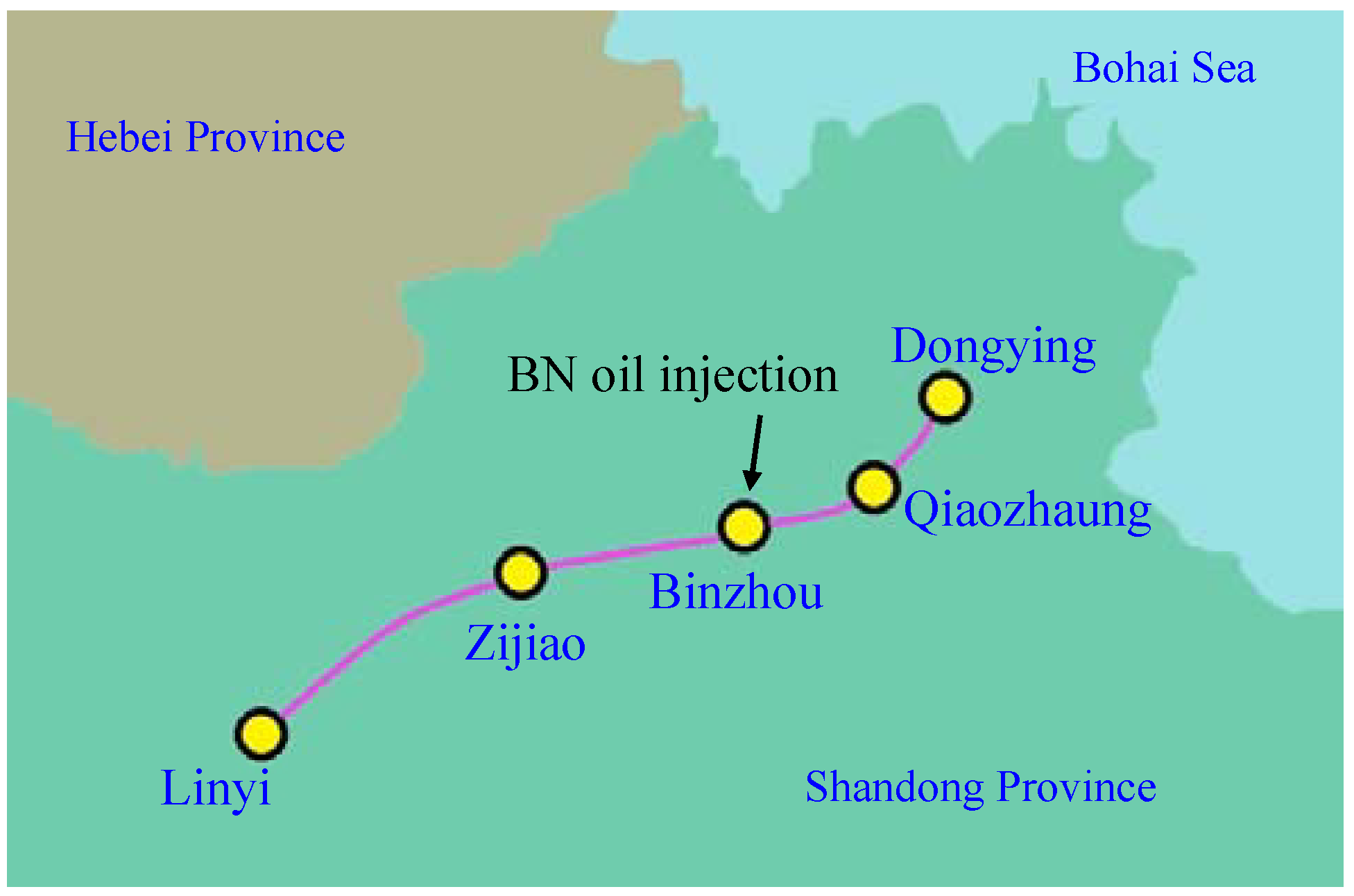
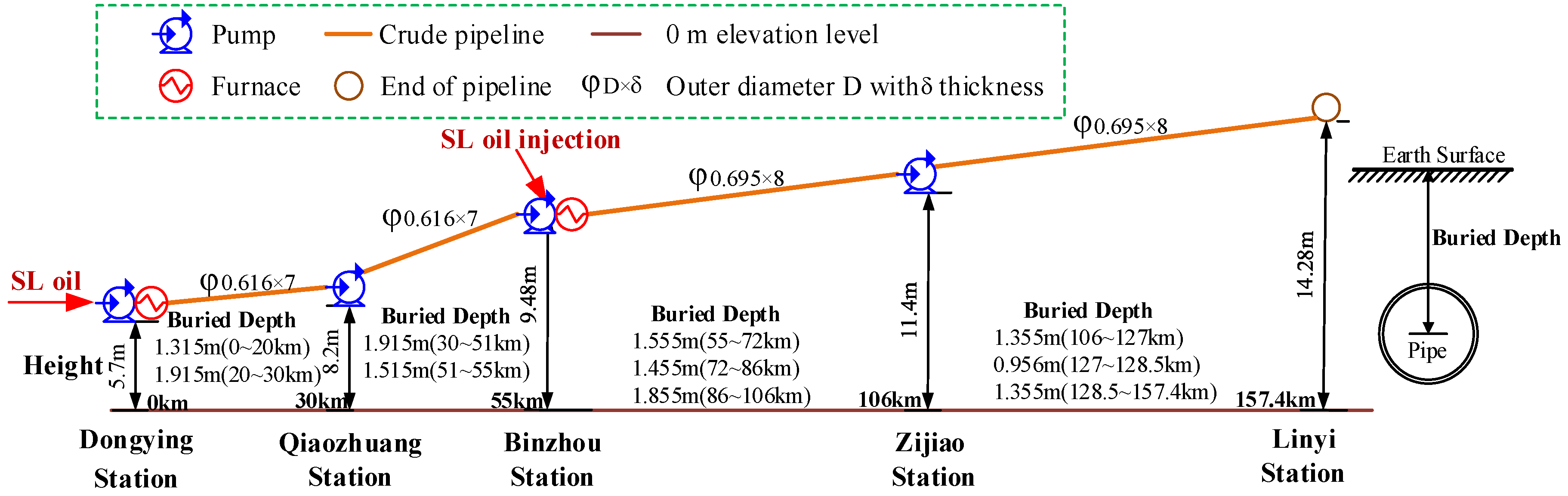
2. Oil Transportation Scheme and Thermal State of Secondary Dong-Lin Pipeline
2.1. Basic Situation
2.2. Thermal State of the Dong-Lin oil Pipeline
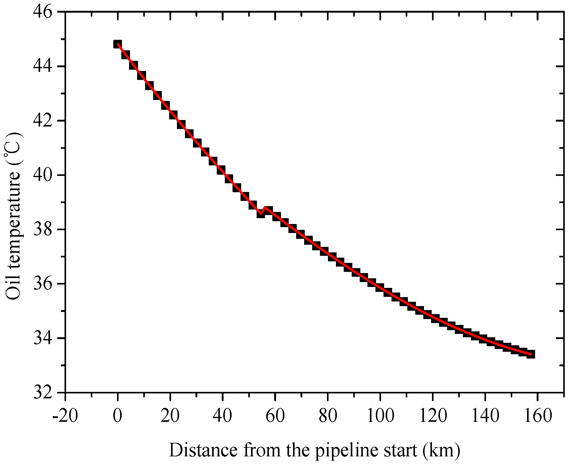
2.2.1. Thermal State before the Batch Transportation

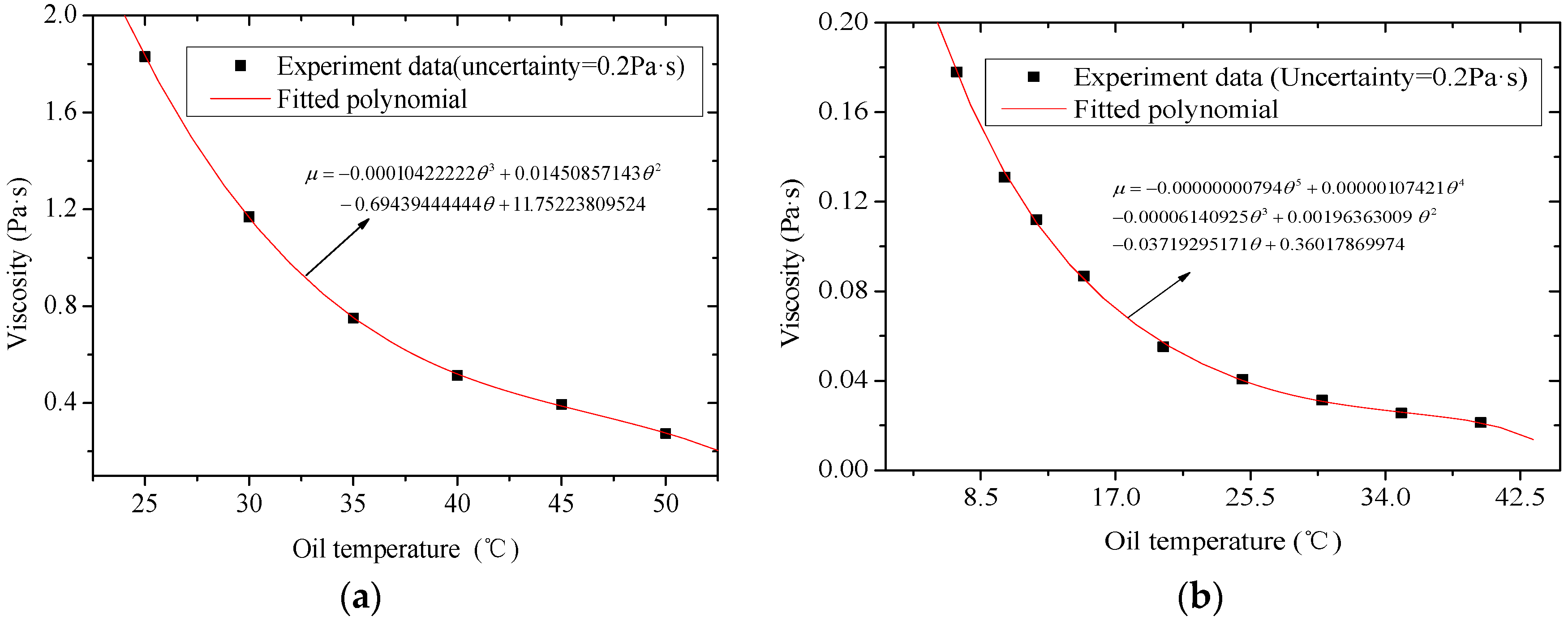
| Oil | (kg/m3) | (J/kg·°C) | (°C) | (Pa·s) |
|---|---|---|---|---|
| SL oil | 937 | 2000 | 11 | Polynomial See Figure 4 |
| OM oil | 868 | 2100 | 0 | |
| SLOM oil | Can be predicted through properties of SL oil and OM oil by equations in Ref. [22]. Sinopec also did extensive testing on the SLOM oil with different ratios of SL and OM oil. | |||
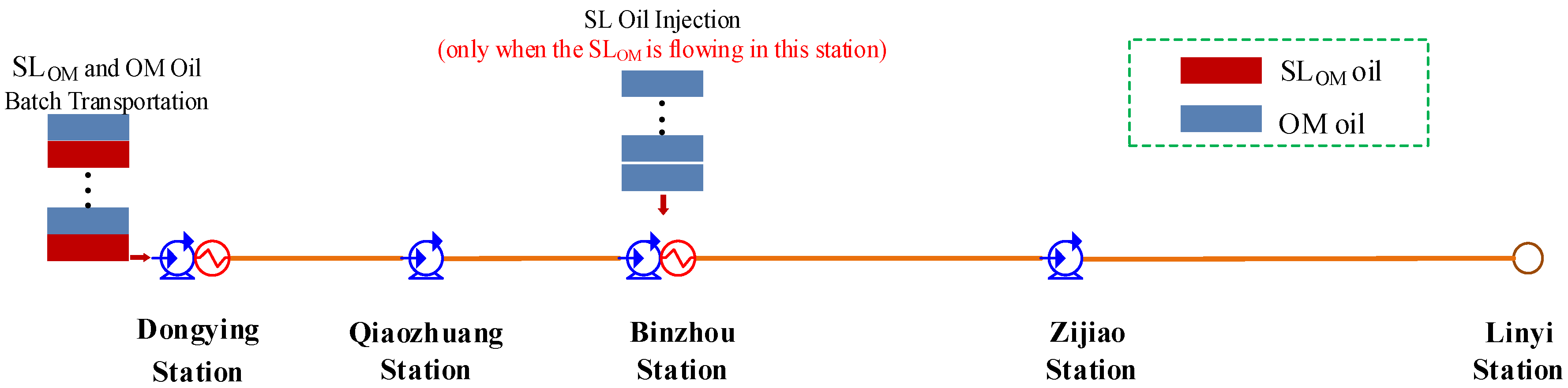
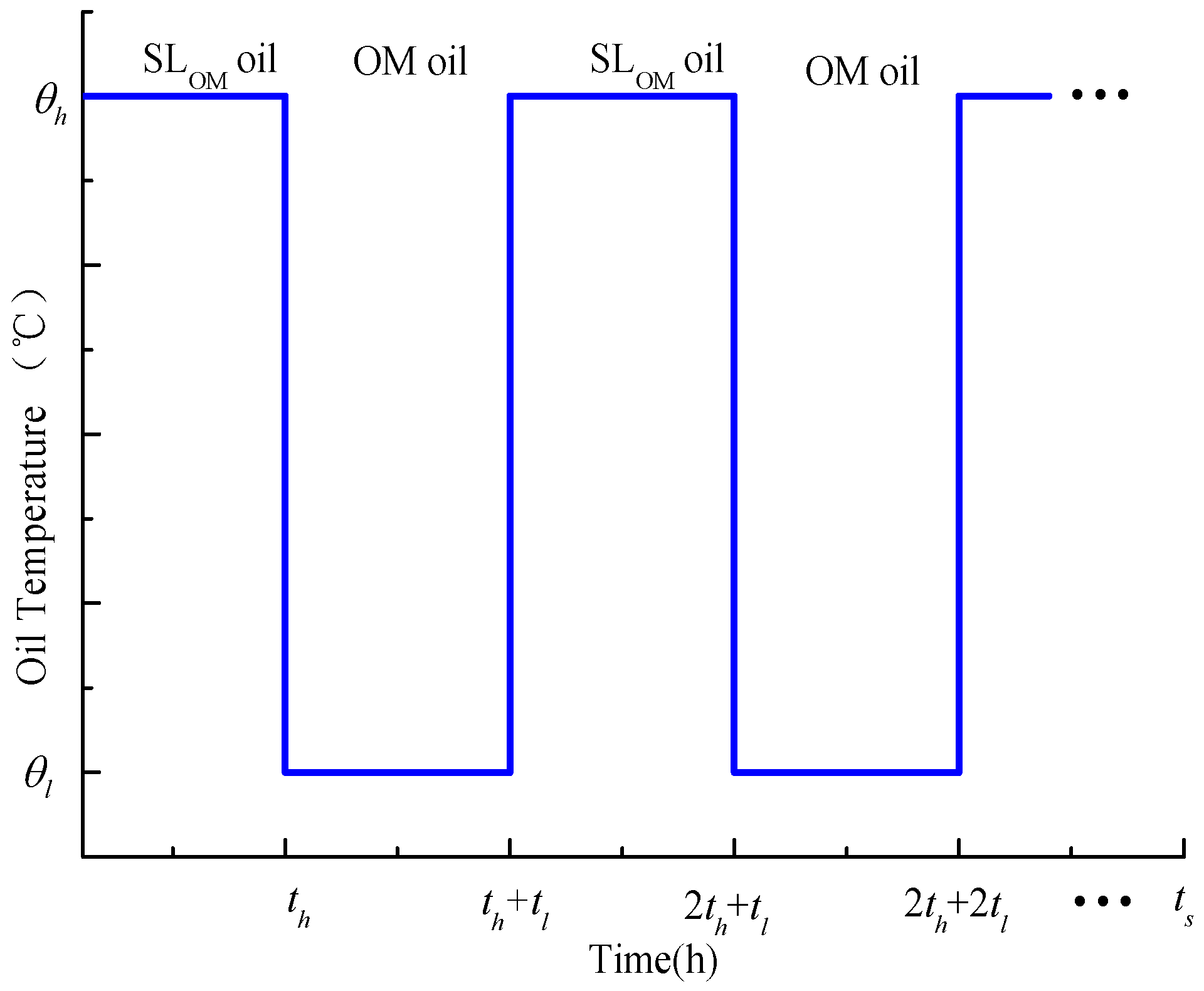
2.2.2. Thermal State of the Batch Transportation
2.3. Detailed Batch Transportation Scheme to be Determined
3. Physical and Mathematical Model for Secondary Dong-Lin Pipeline
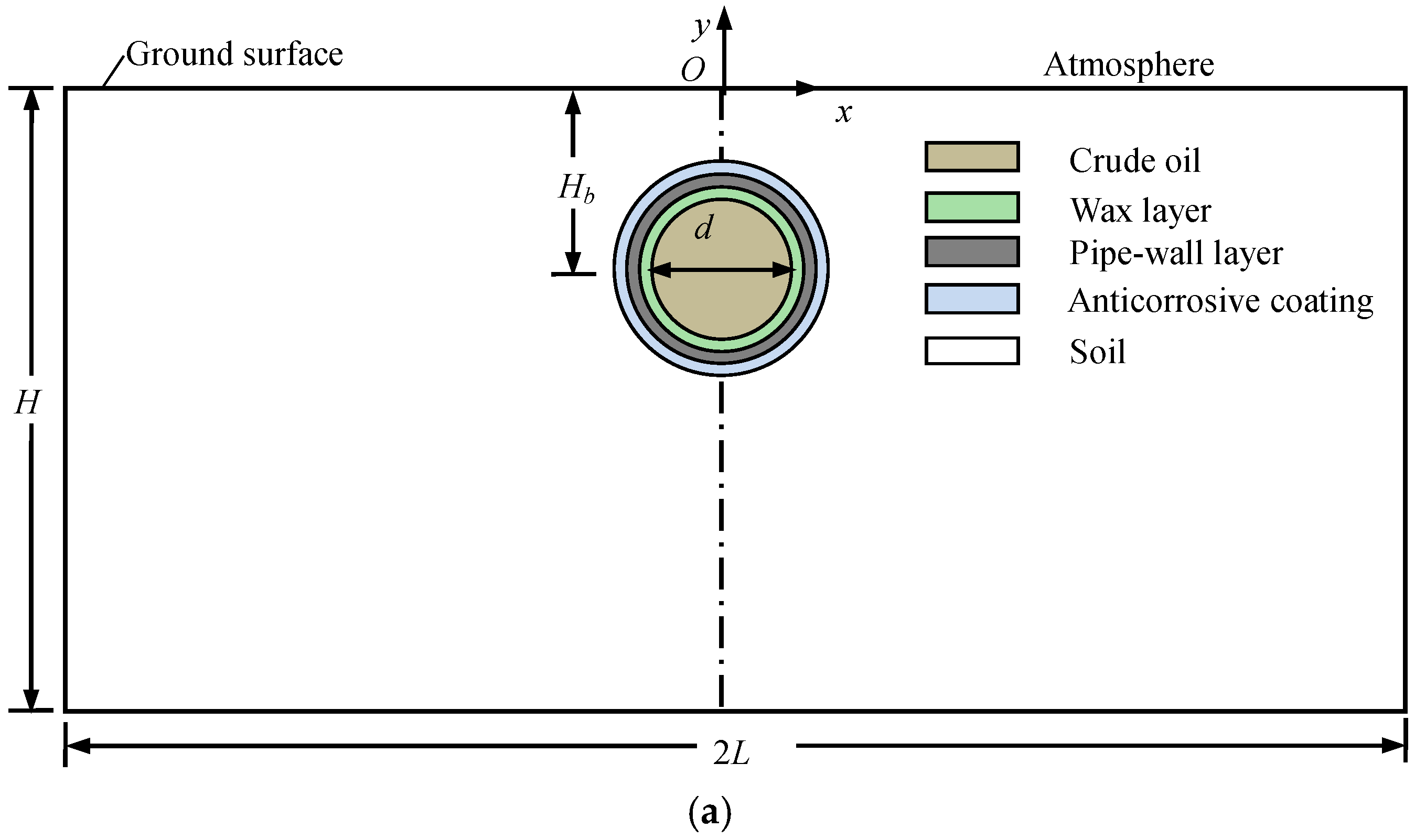
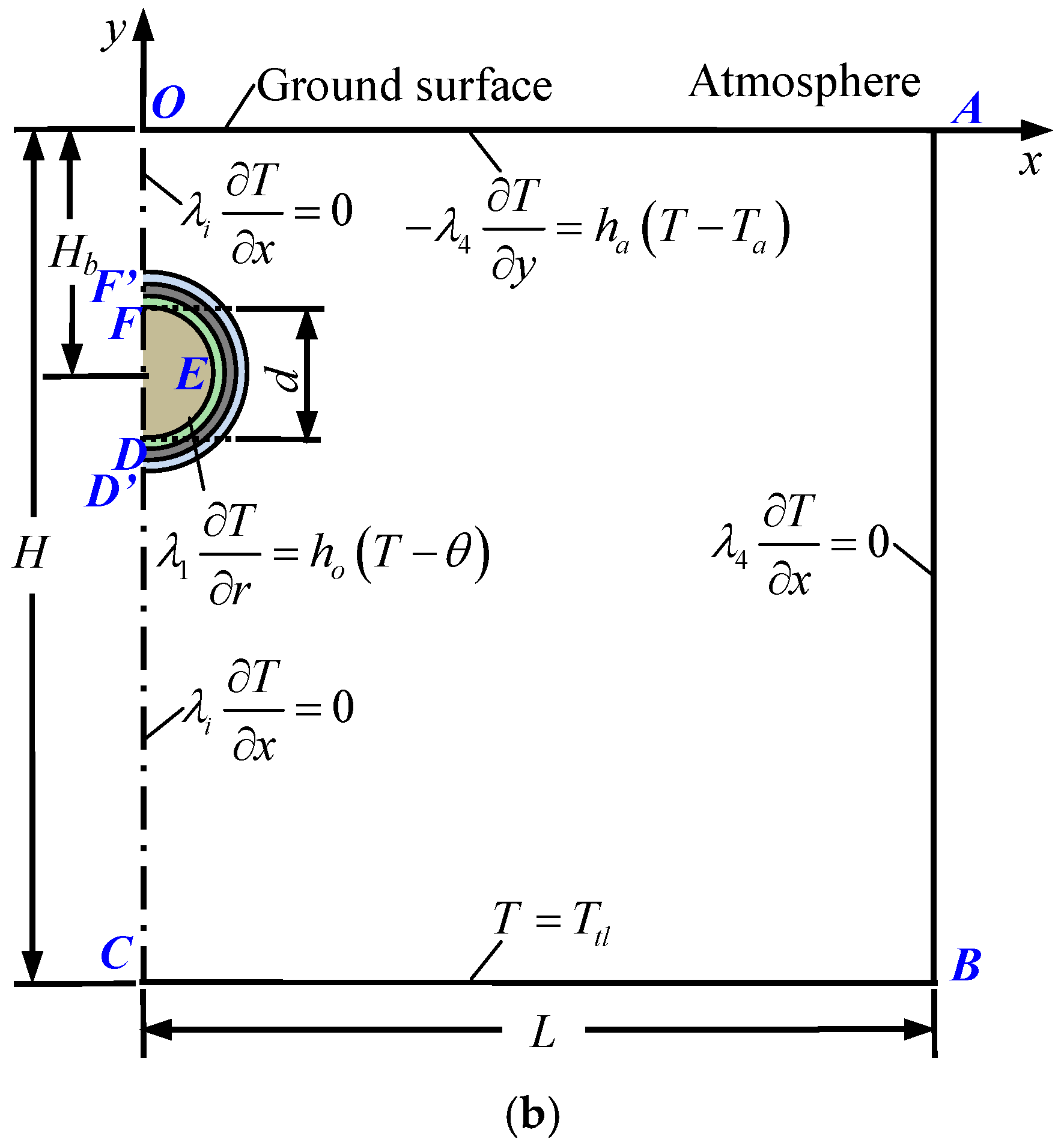
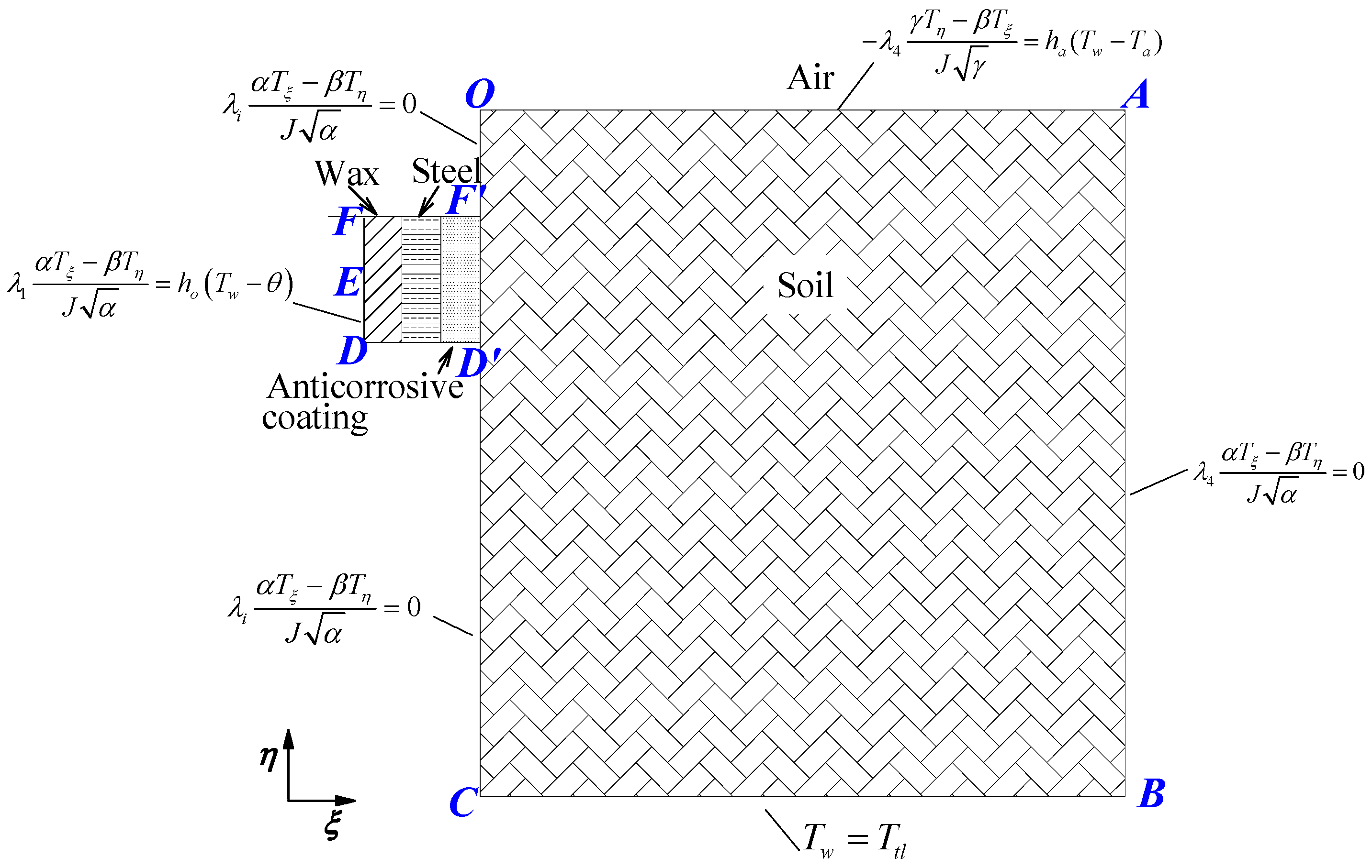
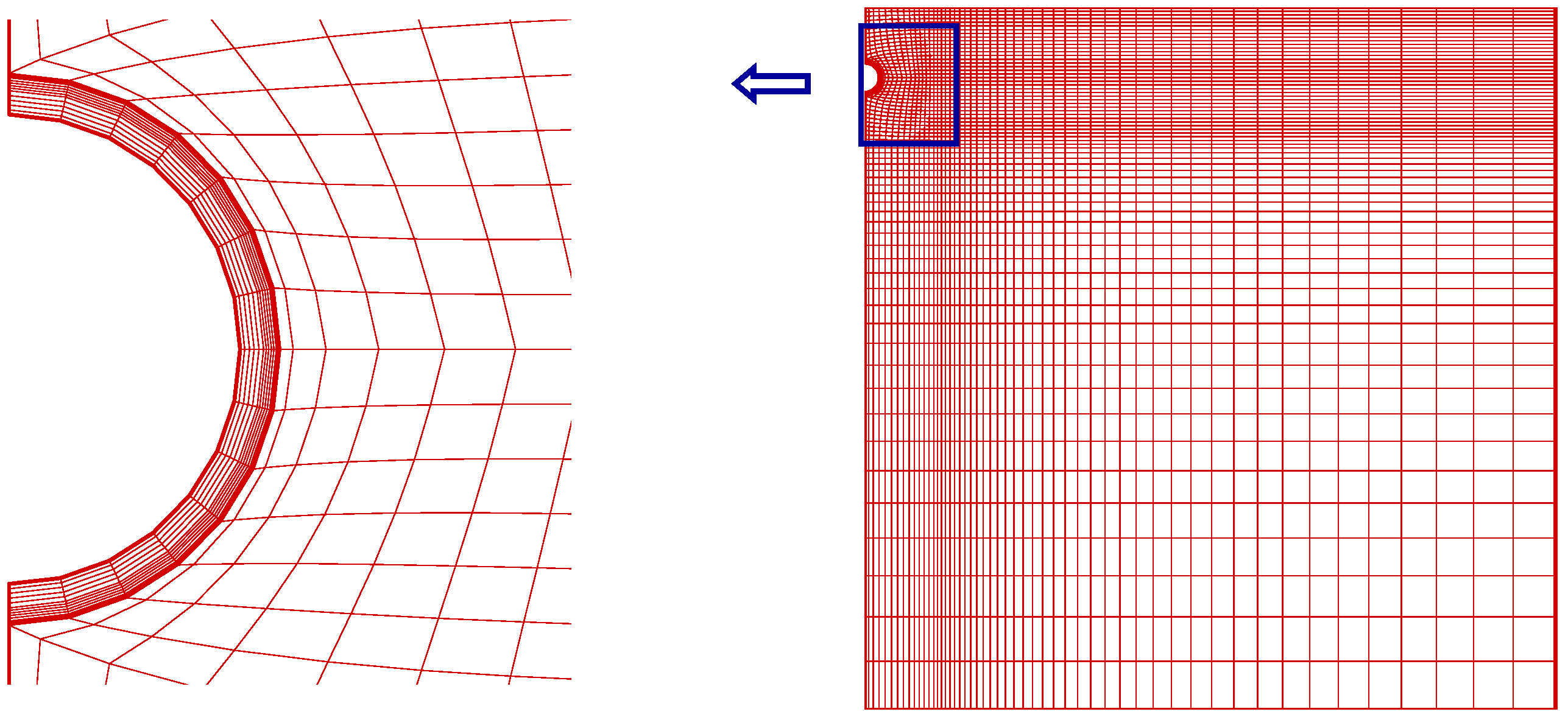
3.1. Physical and Mathematical Model of the Pipeline Cross-section
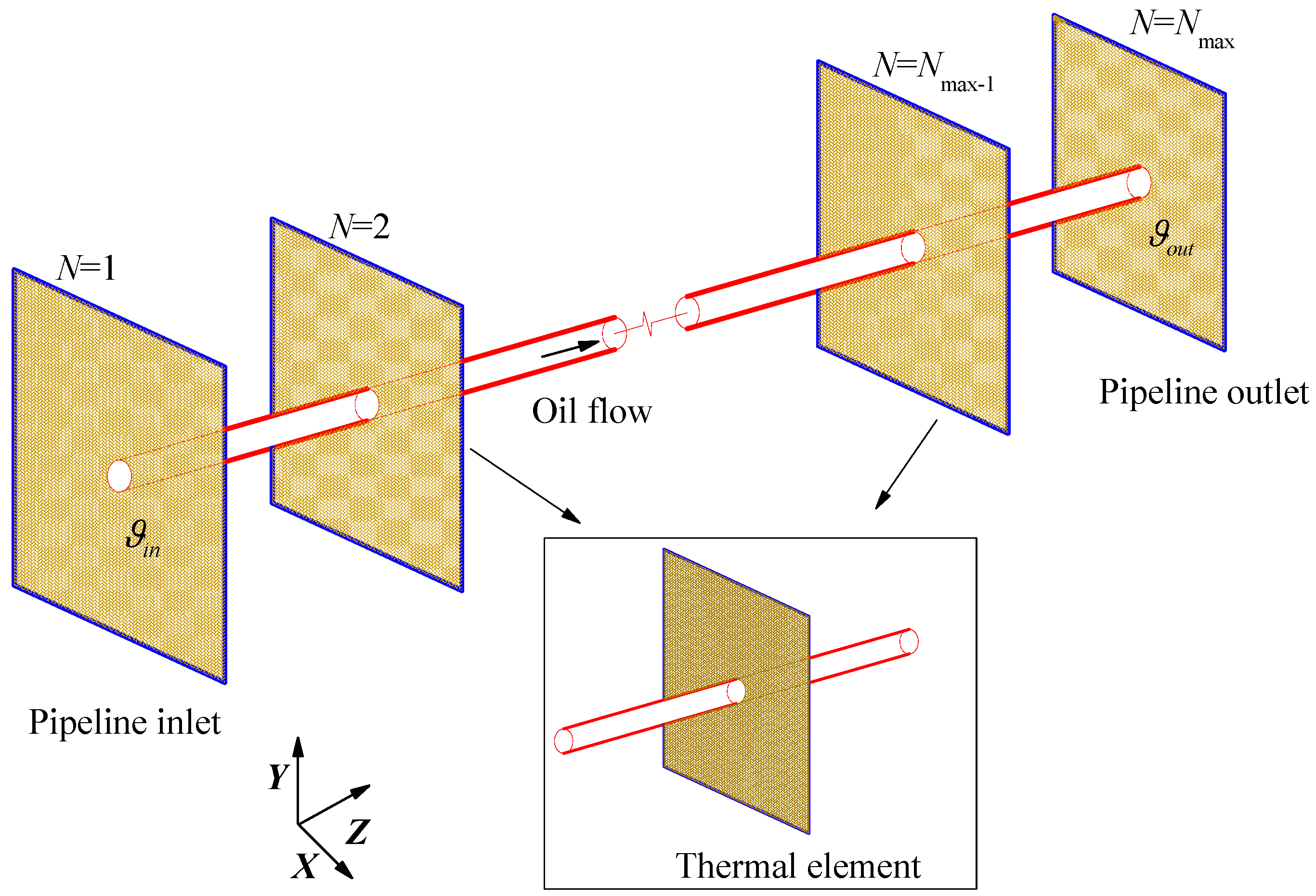
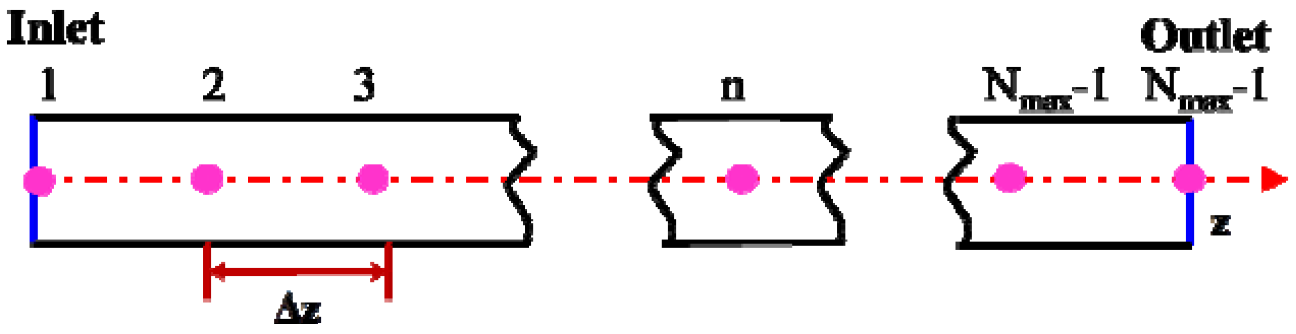
3.2. Physical and mathematical model of the oil stream
4. Model Reduction for Pipeline’s Cross-section Thermal Simulation
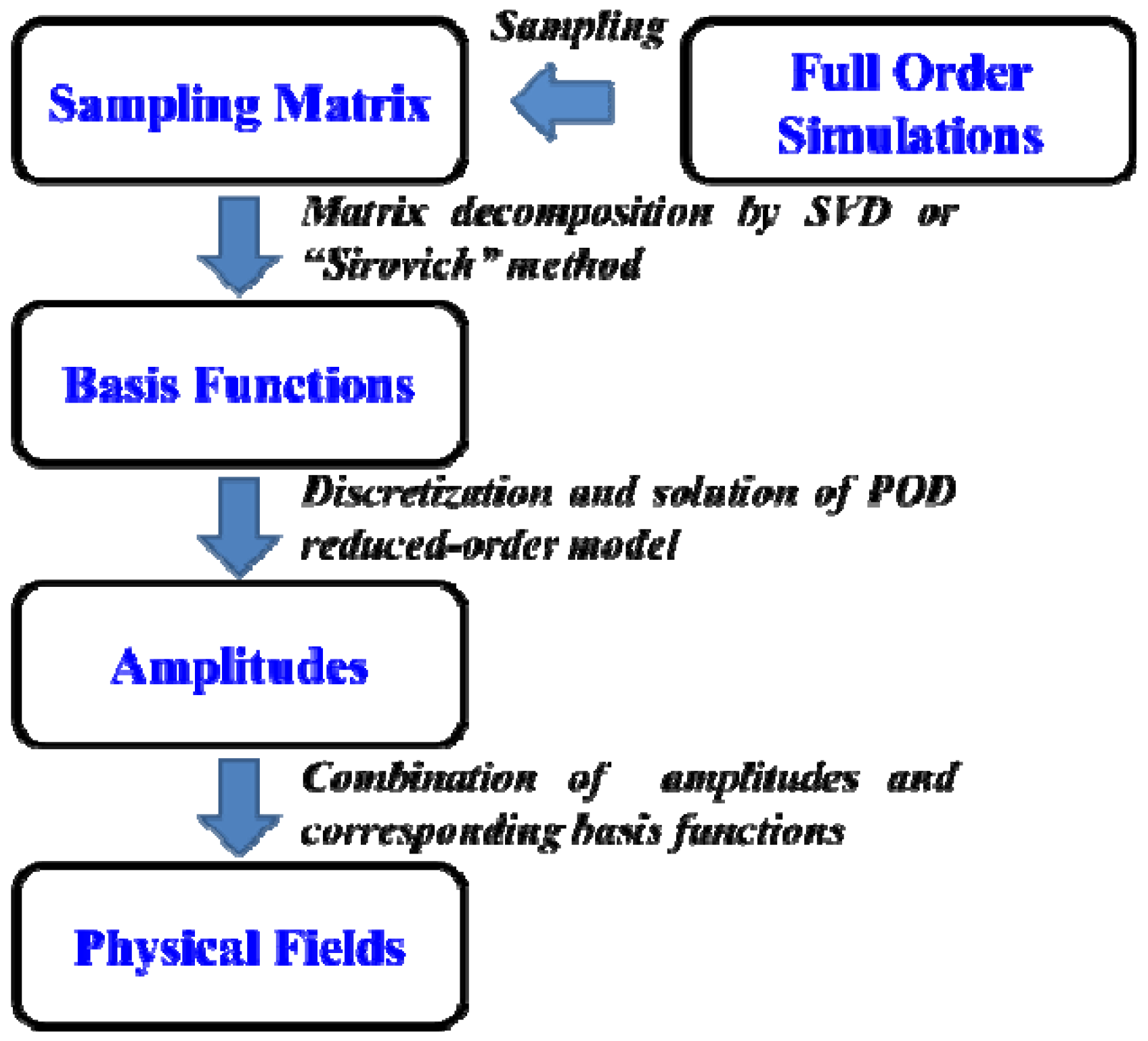
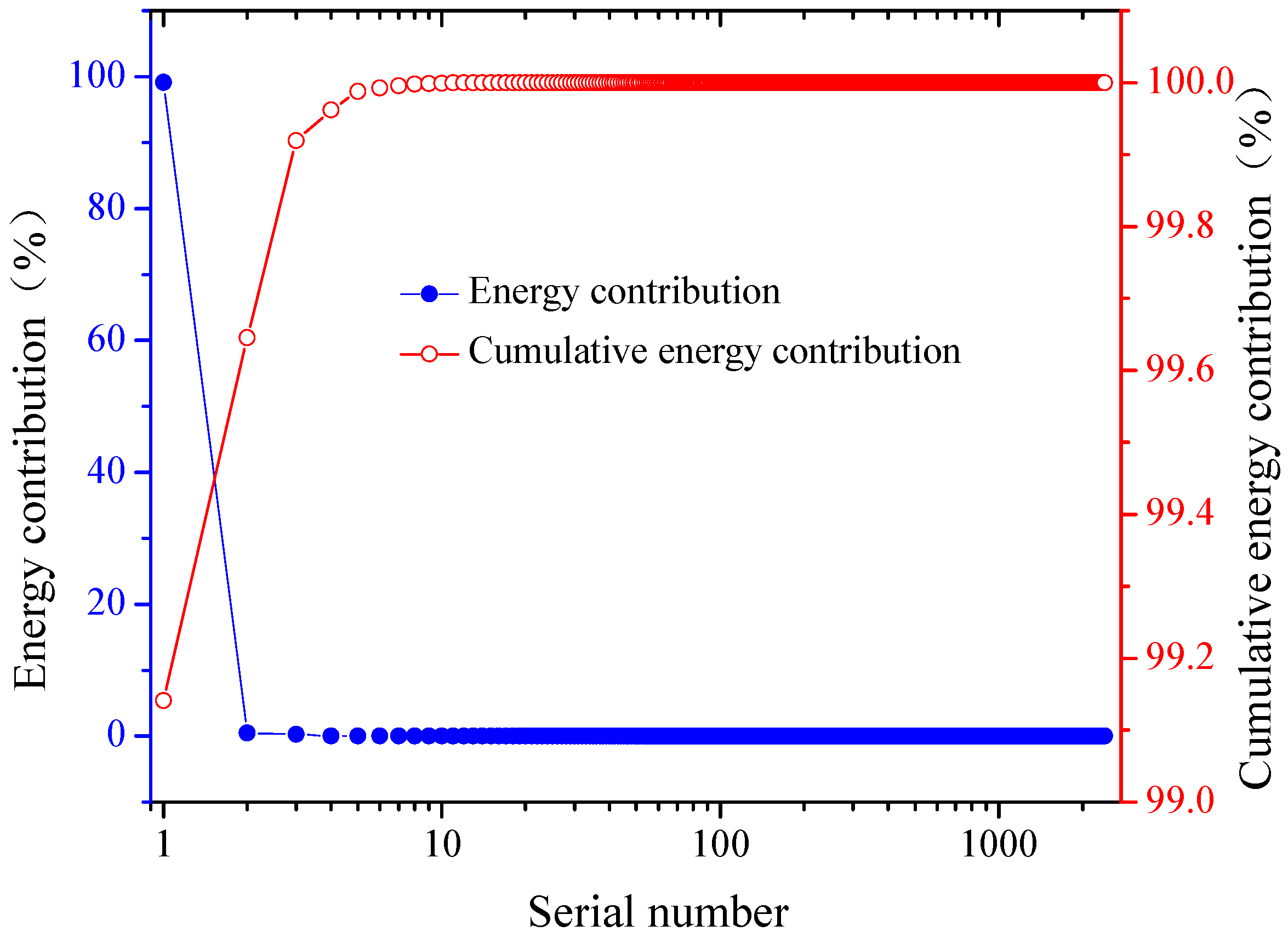
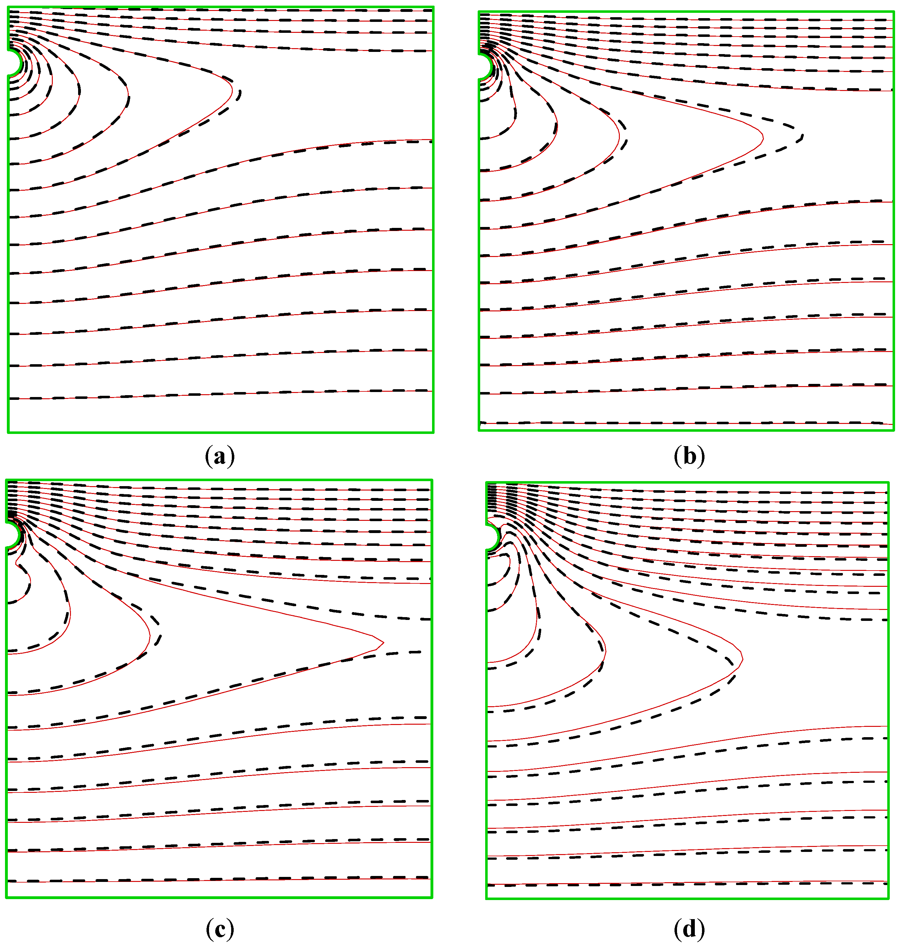
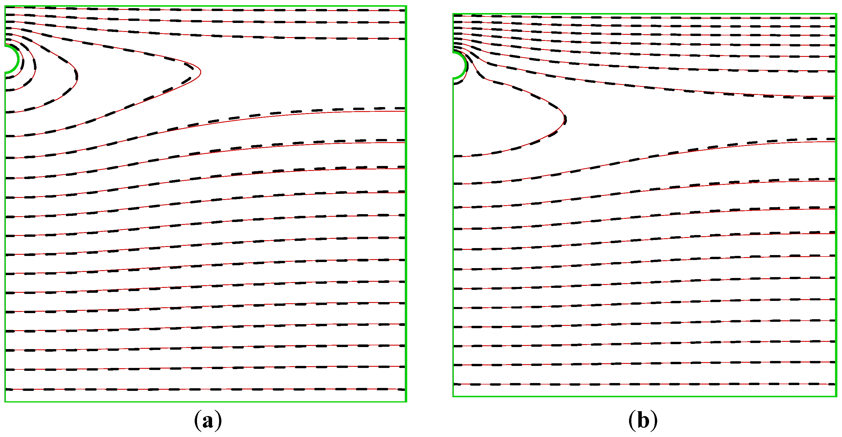
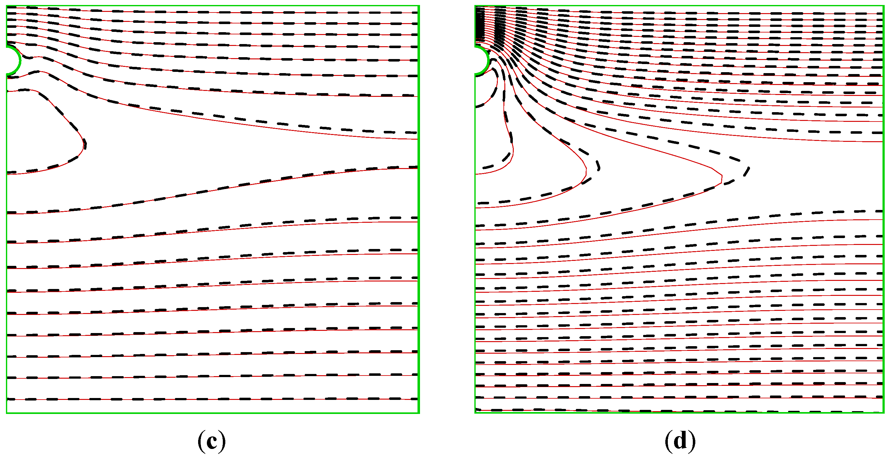
4.1. POD Basis Function
4.2. Reduced-order model (equations of )
- .
4.3. The standard POD reduced-order model implementation procedure
5. Application and Discussions
5.1. Property and Boundary Variables for Secondary Dong-Lin crude Pipeline
- (1)
- Property parameters
- (2)
- Boundary parameters
5.2. POD-ROM-based fast thermal simulation for Secondary Dong-Lin crude pipeline
5.2.1. Sampling and Basis function
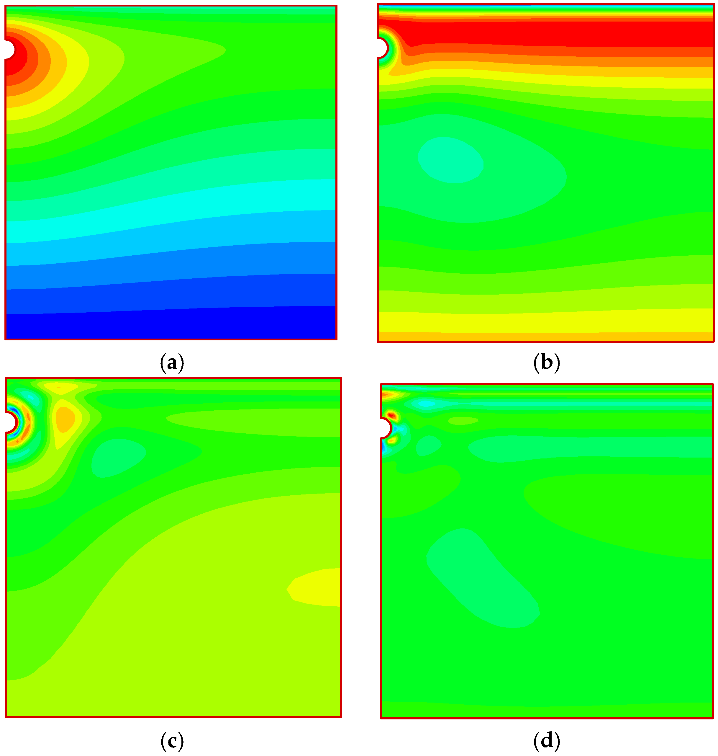
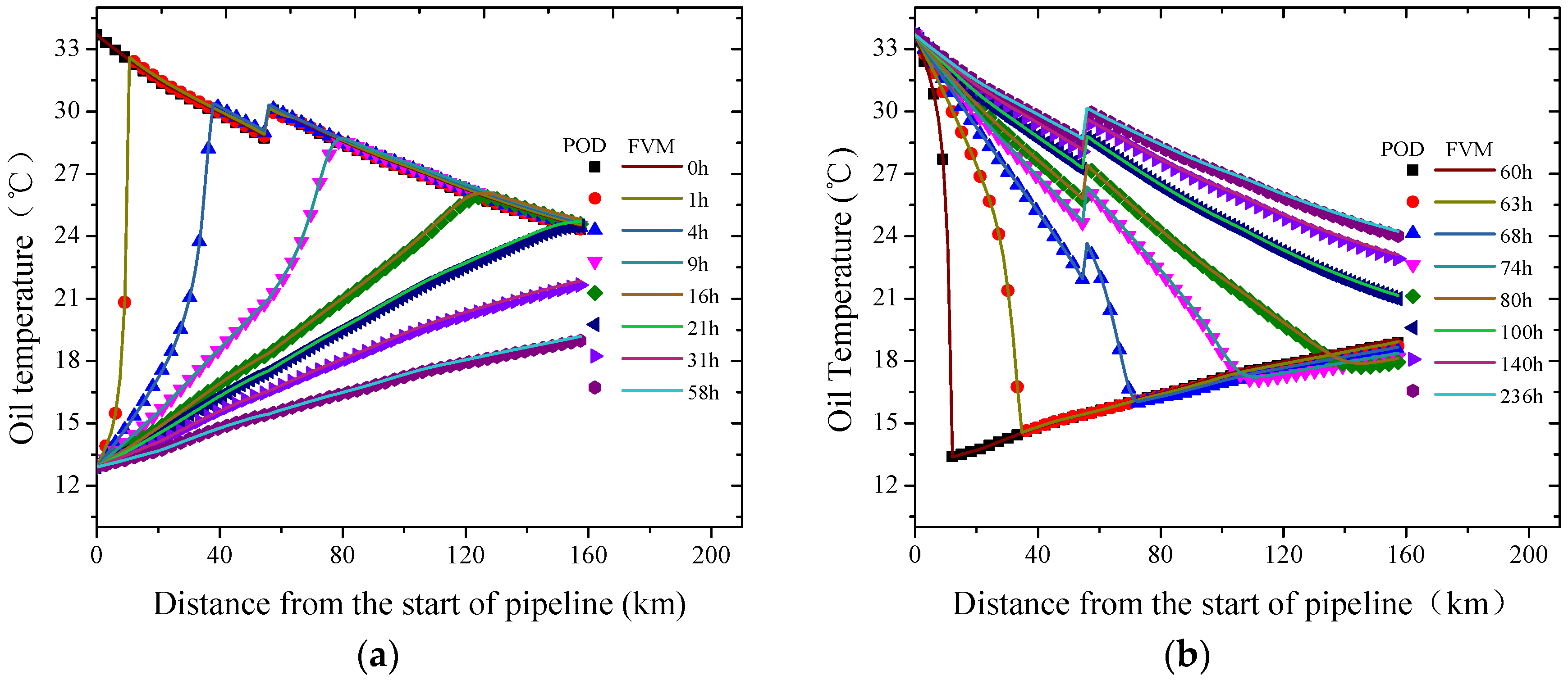
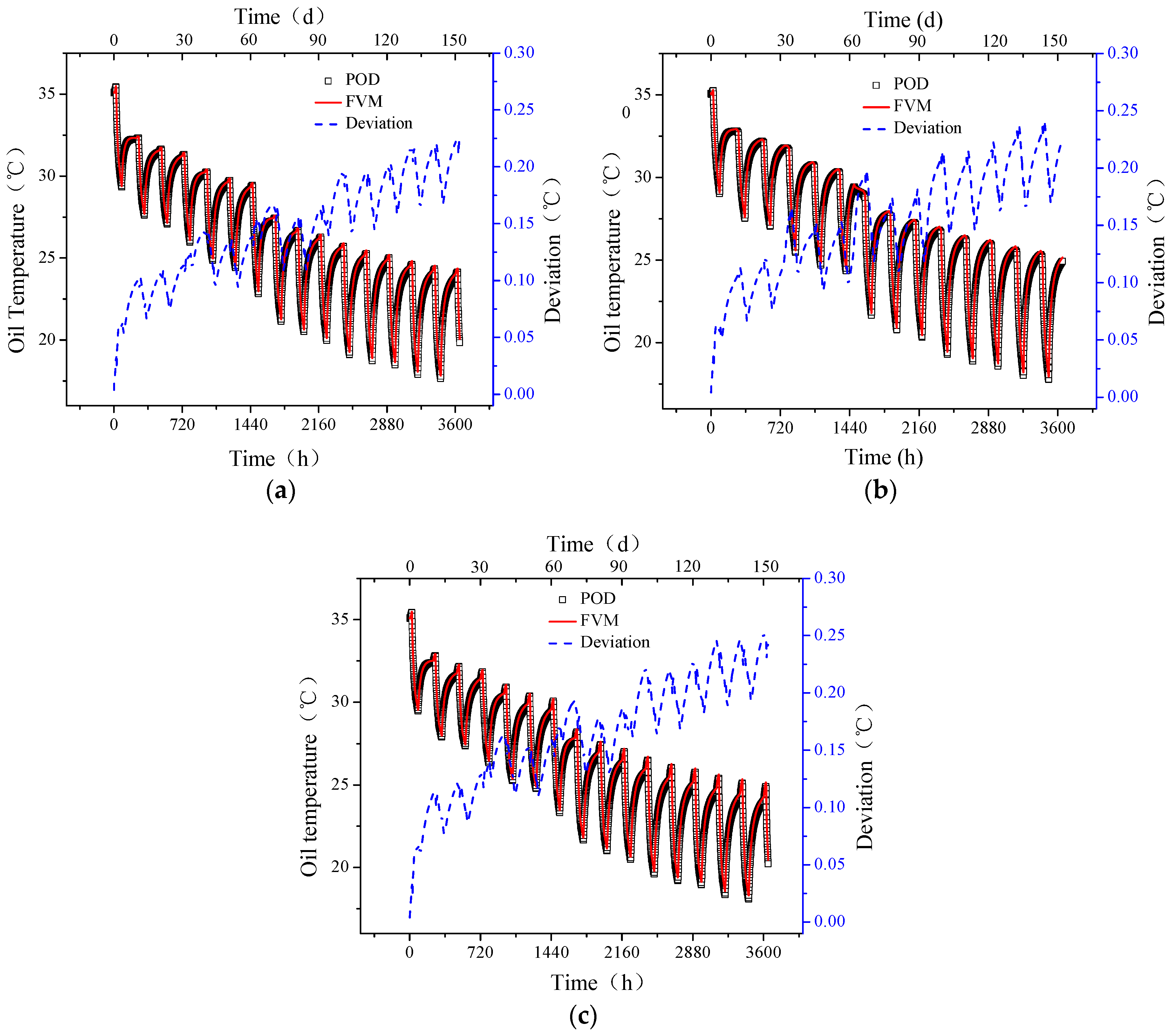
5.2.2. POD Reduced-order model validation and thermal characteristics of batch transportation
5.3. Detail Batch Transportation Scheme Determination and Field Verification
| Scheme No. | (m3h−1/m3h−1) | (m3h−1) | (°C/°C) | (d/d) | |
|---|---|---|---|---|---|
| 124 | 1370/2064 | 172 | See Table 11 | 4.58/1.17 | 9:2 |
6. Conclusions
- (1)
- Sampling matrix construction and basis function obtainment.
- (2)
- The validation of the POD reduced-order model.
- (3)
- The determination of the transportation scheme.
Author Contributions
Funding
Conflicts of Interest
Nomenclature
| Roman Symbols | |
| Amplitude of the kth POD basis function | |
| Flowing area of the pipeline (m2) | |
| Specific heat capacity of region i (J/(kg·°C)) | |
| Specific heat capacity of oil (J/(kg·°C)) | |
| Diameter of the pipeline (mm) | |
| The Darcy coefficient | |
| Heat convection coefficient between the wax layer and oil stream (W/(m2·°C)) | |
| Heat convection coefficient between the soil and air (W/(m2·°C)) | |
| Thermal influence region on the vertical direction (m) | |
| The buried depth of crude oil pipeline (m) | |
| Thermal influence region on the horizontal direction (m) | |
| The heat flux between the wax layer and oil stream (W/m2) | |
| Flow flux of hot and cool oil in Dongying station (m3/h) | |
| The flow flux injected in Binzhou station (m3/h) | |
| Ratio of SL oil and OM oil in SLOM oil | |
| The sampling matrix | |
| Transportation time of hot oil during one period (h) | |
| Transportation time of cool oil during one period (h) | |
| The total transportation time of hot and cool oils (h) | |
| Temperature of the pipeline’s cross-section | |
| Temperature of the air (°C) | |
| Temperature of the soil thermostat layer (°C) | |
| Flow velocity of the oil stream (m/s) | |
| Cartesian coordinate in the cross-section of pipeline (m) | |
| Coordinate along the cross-section of pipeline (m) | |
| Greek Symbols | |
| Thickness of the wax layer (m) | |
| Thickness of the anticorrosive layer (m) | |
| The kth POD basis function | |
| Vector of the kth POD basis function | |
| Heat conductivity coefficient of region i (W/(m·°C) ) | |
| Viscosity (Pa·s) | |
| Temperature of the oil (°C) | |
| Condensation point of crude oil (°C) | |
| Temperature of the hot oil, namely SLOM oil (°C) | |
| Temperature of the cool oil, namely OM oil (°C) | |
| Temperature of SLOM oil (°C) | |
| Temperature of OM oil (°C) | |
| Density of region i (W/(m·°C) ) | |
| Density of oil (kg/m3) | |
| Body-fitted coordinate in the cross-section of pipeline (m) | |
| Subscripts | |
| 1,2,3,4 | Regions of wax layer, pipe-wall layer, anticorrosive layer and soil respectively |
| ac | Anticorrosive layer |
| h | Hot oil |
| l | Cool oil, namely low temperature oil |
| o | oil |
| OM | Oman oil |
| SL | Shengli oil |
| SLOM | Mixture of SL oil and OM oil |
| tl | Thermostat layer |
| w | Wax layer |
| Partial derivatives of the variable | |
References
- Yu, Y.; Wu, C.; Xing, X.; Zuo, L. Energy saving for a Chinese crude oil pipeline. In Proceedings of the ASME 2014 Pressure Vessels and Piping Conference, Garden Grove, CA, USA, 20–24 July 2014. [Google Scholar] [CrossRef]
- Zhang, H.R.; Liang, Y.T.; Xia, Q.; Wu, M.; Shao, Q. Supply-based optimal scheduling of oil product pipelines. Petrol. Sci. 2016, 13, 355–367. [Google Scholar] [CrossRef]
- Shauers, D.; Sarkissian, H.; Decker, B. California line beats odds, begins moving viscous crude oil. Oil Gas J. 2000, 98, 54–66. [Google Scholar]
- Mecham, T.; Wikerson, B.; Templeton, B. Full Integration of SCADA, field control systems and high speed hydraulic models-application Pacific Pipeline System. In Proceedings of the International Pipeline Conference, Calgary, AB, Canada, 1–5 October 2000. [Google Scholar] [CrossRef]
- Cui, X.G.; Zhang, J.J. The research of heat transfer problem in process of batch transportation of cool and hot oil. Oil Gas Stor. Trans. 2013, 23, 15–19. [Google Scholar] [CrossRef]
- Wang, K.; Zhang, J.J.; Yu, B.; Zhou, J.; Qian, J.H.; Qiu, D.P. Numerical simulation on the thermal and hydraulic behaviors of batch pipelining crude oils with different inlet temperatures. Oil Gas Sci. Technol. 2009, 64, 503–520. [Google Scholar] [CrossRef]
- Yuan, Q.; Wu, C.C.; Yu, B.; Han, D.; Zhang, X.; Cai, L.; Sun, D. Study on the thermal characteristics of crude oil batch pipelining with differential outlet temperature and inconstant flow rate. J. Petrol. Sci. Eng. 2018, 160, 519–530. [Google Scholar] [CrossRef]
- Lumley, J.L. The Structure of Inhomogeneous Turbulent Flows in Atmospheric Turbulence and Radio Wave Propagation; Nauka: Moscow, Russian, 1967. [Google Scholar]
- Sirovich, L. Turbulence and dynamics of coherent structures, Part 1: Coherent structures. Q. Appl. Math. 1987, 45, 561–571. [Google Scholar] [CrossRef]
- Huang, N.E.; Shen, Z.; Long, S.R.; Wu, M.L.; Shih, H.H.; Zheng, Q.; Yen, N.C.; Tung, C.C.; Liu, H.H. The empirical mode decomposition and Hilbert spectrum for nonlinear and nonstationary time series analysis. Proc. Roy. Soc. London A 1998, 454, 903–995. [Google Scholar] [CrossRef]
- Schmid, P.J. Dynamic mode decomposition of numerical and experimental data. J. Fluid Mech. 2010, 656, 5–28. [Google Scholar] [CrossRef]
- Banerjee, S.; Cole, J.V.; Jensen, K.F. Nonlinear model reduction strategies for rapid thermal processing systems. IEEE Trans. Semiconduct. Manuf. 1988, 11, 266–275. [Google Scholar] [CrossRef]
- Raghupathy, A.P.; Ghia, U. Boundary-condition-independent reduced-order modeling of complex 2D objects by POD-Galerkin methodology. In Proceedings of the IEEE Semiconductor Thermal Measurement and Management Symposium, San Jose, CA, USA, 15–19 March 2009. [Google Scholar] [CrossRef]
- Fogleman, M.; Lumley, J.; Rempfer, D.; Haworth, D. Application of the proper orthogonal decomposition to datasets of internal combustion engine flows. J. Turbul. 2004, 5, 1–18. [Google Scholar] [CrossRef]
- Ding, P.; Tao, W.Q. Reduced order model based algorithm for inverse convection heat transfer problem. J. Xi’an Jiaotong Univ. 2009, 43, 14–16. [Google Scholar] [CrossRef]
- Thomas, A.B.; Raymond, L.F.; Pau, G.A.; Thomas, J.; Breault, R.W. A reduced-order model for heat transfer in multiphase flow and practical aspects of the proper orthogonal decomposition. Theor. Comp. Fluid Dyn. 2012, 43, 68–80. [Google Scholar] [CrossRef]
- Gaonkar, A.K.; Kulkarni, S.S. Application of multilevel scheme and two level discretization for POD based model order reduction of nonlinear transient heat transfer problems. Comput. Mech. 2015, 55, 179–191. [Google Scholar] [CrossRef]
- Selimefendigil, F.; Öztop, F. Numerical study of natural convection in a ferrofluid-filled corrugated cavity with internal heat generation. Numer. Heat Tr. A-Appl. 2015, 67, 1136–1161. [Google Scholar] [CrossRef]
- Han, D.; Yu, B.; Yu, G.; Zhao, Y.; Zhang, W. Study on a BFC-based POD-Galerkin ROM for the steady-state heat transfer problem. Int. J. Heat Mass Tran. 2014, 69, 1–5. [Google Scholar] [CrossRef]
- Han, D.; Yu, B.; Zhang, X. Study on a BFC-Based POD-Galerkin Reduced-Order Model for the unsteady-state variable-property heat transfer problem. Numer. Heat Tr. B-Fund. 2014, 65, 256–281. [Google Scholar] [CrossRef]
- Yu, G.; Yang, Q.; Dai, B.; Fu, Z.; Lin, D. Numerical study on the characteristic of temperature drop of crude oil in a model oil tanker subjected to oscillating motion. Energies 2018, 11, 1229. [Google Scholar] [CrossRef]
- Yang, Y.H. Design and Management of Oil Pipeline, 1st ed.; Press of China Petroleum University: Qing Dao, China, 2006. [Google Scholar]
- Cheng, Q.; Gan, Y.; Su, W.; Liu, Y.; Sun, W.; Xu, Y. Research on exergy flow composition and exergy loss mechanisms for waxy crude oil pipeline transport processes. Energies 2017, 10, 1956. [Google Scholar] [CrossRef]
- Tao, W.Q. Numerical Heat Transfer; Xi’an Jiaotong University Press: Xi’an, China, 2001. [Google Scholar]


| Soil and the three layers | (kg/m3) | (J/kg·°C) | (W/m·°C) |
|---|---|---|---|
| Soil (0 km–56 km) | 2235 | 1.67 | 943 |
| Soil (56 km–157.4 km) | 2235 | 1.35 | 943 |
| Anticorrosive Layer | 1000 | 0.4 | 1670 |
| Pipe-wall Layer | 7850 | 50 | 460 |
| Wax Layer | 1000 | 0.15 | 2000 |
| Soil Temperature in Buried Depth (°C) | |||||
|---|---|---|---|---|---|
| Date | 0 km | 30 km | 55 km | 106 km | 157.4 km |
| Oct. 31st 2015 | 22.67 | 22.44 | 20.28 | 20.75 | 24.76 |
| Nov. 30th 2015 | 15.90 | 19.39 | 14.89 | 17.31 | 21.09 |
| Dec. 31st 2015 | 7.39 | 13.39 | 9.94 | 12.71 | 15.68 |
| Jan. 31st 2016 | 5.86 | 11.27 | 8.03 | 9.33 | 13.02 |
| Feb. 29th 2016 | 5.23 | 10.14 | 7.24 | 8.32 | 11.31 |
| Sampling No. | Geometry (See Table 5) | (°C) | (W/m·°C) | (°C) | (°C) | (d/d) | Tinitial (°C) | (d) |
|---|---|---|---|---|---|---|---|---|
| 1 | Geo1 | See Table 6 | 1.67 | 23 | 38 | 1.5/3.5 | 0 | 50 |
| 2 | Geo2 | 20 | 38 | 45 | ||||
| 3 | Geo3 | 1.35 | 15 | 35 | 0.5/1.5 | 75 | ||
| 4 | Geo4 | 14 | 36 | 105 | ||||
| 5 | Geo5 | 13 | 35 | 157 |
| Geo No. | (m) | (m) | (m) | (m) |
|---|---|---|---|---|
| Geo 1 | 1.315 | 0.003 | 0.007 | |
| Geo2 | 1.915 | 0.003 | 0.007 | |
| Geo3 | 1.3555 | 0.003 | 0.007 | |
| Geo4 | 1.5555 | 0.003 | 0.007 | |
| Geo5 | 1.8555 | 0.003 | 0.007 |
| Time | 0 d–10 d | 10 d–20 d | 20 d–30 d | 30 d–40 d | 40 d–50 d |
|---|---|---|---|---|---|
| (°C) | 22.67 | 15.9 | 7.39 | 5.86 | 5.23 |
| Scheme No. | (m3h−1/m3h−1) | (m3h−1) | (°C/°C) | (d/d) | |
|---|---|---|---|---|---|
| 1 | 2161/2470 | 172 | See Table 8 | 7.56/2.44 | 90:36 |
| 2 | 2322/2321 | 8.11/2.83 | 90:26 | ||
| 3 | 1872/2470 | 7.56/2.44 | 90:20 |
| Time | (°C) | (°C) | Furnaces | ||
|---|---|---|---|---|---|
| Scheme 1 | Scheme 2 | Scheme 3 | |||
| Oct. 2015 | 23.20 | 37.03 | 38.22 | 39.04 | Both furnaces in Dongying and Binzhou are closed |
| Nov. 2015 | 20.00 | 36.37 | 37.78 | 38.75 | |
| Dec. 2015 | 14.88 | 33.77 | 35.39 | 36.51 | |
| Jan. 2016 | 13.60 | 33.89 | 35.64 | 36.84 | |
| Feb. 2016 | 12.90 | 33.69 | 35.48 | 36.71 | |
| Scheme No. | FVM (h) | POD (h) | Acceleration Factor |
|---|---|---|---|
| Scheme 1 | 62.7 | 0.49 | 128 |
| Scheme 2 | 64.5 | 0.52 | 124 |
| Scheme 3 | 64.0 | 0.56 | 114 |
| Time | (°C) | (°C) | Furnace in Dongying | Furnace in Linyi |
|---|---|---|---|---|
| Oct. 2015 | 23.5 | 41.5 | Close for OM oil. Open for SLOM oil and keep heating it to 41.5 °C | Open for both OM and SLOM oil Raise OM oil 8 °C Raise SLOM oil 5 °C |
| Nov. 2015 | 23 | 41.5 | ||
| Dec. 2015 | 21 | 41.5 | ||
| Jan. 2016 | 19 | 41.5 | ||
| Feb. 2016 | 17 | 41.5 |
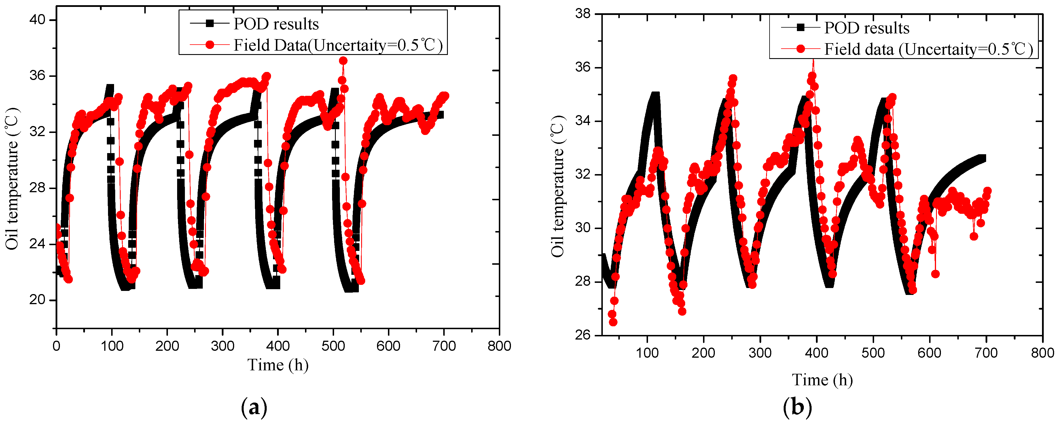
| Oil | Data | Nov. 2015 | Dec. 2015 | Jan. 2016 | Feb. 2016 | ||||
|---|---|---|---|---|---|---|---|---|---|
| in BZ | Field Data | 28.89 | (0.24, 0.8%) | 26.78 | (0.48, 1.8%) | 25.66 | (1.21, 4.7%) | 23.54 | (0.42, 1.8%) |
| POD Results | 29.13 | 26.30 | 24.45 | 23.12 | |||||
| in LY | Field Data | 32.18 | (1.27, 3.9%) | 32.93 | (0.15, 0.4%) | 29.62 | (0.48, 1.6%) | 29.98 | (0.32, 1.1%) |
| POD Results | 33.45 | 33.08 | 30.10 | 30.30 | |||||
| Oil | Data | Nov. 2015 | Dec. 2015 | Jan. 2016 | Feb. 2016 | ||||
|---|---|---|---|---|---|---|---|---|---|
| in BZ | Field Data | 36.02 | (0.12, 0.3%) | 35.66 | (0.48, 1.3%) | 33.89 | (1.21, 3.6%) | 33.64 | (0.06, 0.2%) |
| POD Results | 36.14 | 36.35 | 34.63 | 33.58 | |||||
| in LY | Field Data | 33.99 | (0.99, 2.9%) | 34.48 | (1.37, 4.0%) | 31.29 | (0.79, 2.5%) | 31.72 | (0.63, 2.0%) |
| POD Results | 34.98 | 35.85 | 32.08 | 32.35 | |||||
© 2018 by the authors. Licensee MDPI, Basel, Switzerland. This article is an open access article distributed under the terms and conditions of the Creative Commons Attribution (CC BY) license (http://creativecommons.org/licenses/by/4.0/).
Share and Cite
Han, D.; Yuan, Q.; Yu, B.; Cao, D.; Zhang, G. BFC-POD-ROM Aided Fast Thermal Scheme Determination for China’s Secondary Dong-Lin Crude Pipeline with Oils Batching Transportation. Energies 2018, 11, 2666. https://doi.org/10.3390/en11102666
Han D, Yuan Q, Yu B, Cao D, Zhang G. BFC-POD-ROM Aided Fast Thermal Scheme Determination for China’s Secondary Dong-Lin Crude Pipeline with Oils Batching Transportation. Energies. 2018; 11(10):2666. https://doi.org/10.3390/en11102666
Chicago/Turabian StyleHan, Dongxu, Qing Yuan, Bo Yu, Danfu Cao, and Gaoping Zhang. 2018. "BFC-POD-ROM Aided Fast Thermal Scheme Determination for China’s Secondary Dong-Lin Crude Pipeline with Oils Batching Transportation" Energies 11, no. 10: 2666. https://doi.org/10.3390/en11102666
APA StyleHan, D., Yuan, Q., Yu, B., Cao, D., & Zhang, G. (2018). BFC-POD-ROM Aided Fast Thermal Scheme Determination for China’s Secondary Dong-Lin Crude Pipeline with Oils Batching Transportation. Energies, 11(10), 2666. https://doi.org/10.3390/en11102666