An Improved Grey Model and Scenario Analysis for Carbon Intensity Forecasting in the Pearl River Delta Region of China

Abstract

In this paper, an improved grey model and scenario analysis, GA-GM(1,N) is proposed to forecast the carbon intensity in the Pearl River Delta (PRD) region, one of the most developed regions in China. Moreover, to show the advantage and feasibility of the proposed model, the forecasting results of the GA-GM(1,N) model are compared with that of a single-variable grey model (GM (1,1)) and a multivariable form (GM(1,N)). Data from one sample period (2005–2012) are used to develop the models, and data from another sample period (2013–2015) are used to test them. The mean absolute percentage error (MAPE) is applied to measure the accuracy of prediction. The results show that, of the three models, GA-GM(1,N) produces the best carbon intensity forecasts, with MAPEs of 0.4–1.4% and 0.04–0.4% in the development and testing periods respectively. This indicates that the optimization of the genetic algorithm is effective. The realization of carbon reduction targets in different cities is also explored by combining grey models with scenario analysis. Only Guangzhou could achieve its reduction target under all scenarios, and it can serve as a reference for other cities. Policy recommendations are provided based on these results.

1. Introduction

Greenhouse gases in the atmosphere are the main cause of global warming [1]. A report from the World Bank reveals that global annual carbon emissions in 2013 reached 36 million tons, with China responsible for 29% of the total, while the USA, Europe and India contributed 15%, 10% and 7%, respectively [2]. Intentions to reduce carbon emissions have been signalled by most countries. The USA used 2005 emissions levels as a benchmark and set a greenhouse gas reduction target of 17% by 2020, while the European Union has committed to reduce its greenhouse gas emissions by 20% of the level in 1990 by 2020. China is at an intermediate stage of industrialization, and the growth of its economy still relies on energy consumption [3]. The Chinese government therefore needs to take account of economic development and energy consumption in setting its carbon reduction target. Based on 2005 levels, the carbon emissions per unit GDP (“carbon intensity”) is set to decrease 40–45% by 2020.

Due to significant differences in stage of economic stage, resource endowment, strategic orientation and ecological conditions among the provinces, the national target has been disaggregated to provincial level by government. For instance, in the Thirteenth Five-Year Plan (2016–2020) a 20.5% carbon intensity reduction target was set for to Guangdong.

Furthermore, there are marked regional differences in levels of economic development within Guangdong Province [4]. As one of the most industrially developed areas of China with nine cities, the Pearl River Delta is responsible for about 85% of Guangdong’s GDP [5]. Its rapid economic growth has been accompanied by huge levels of energy consumption as well as serious environmental problems. According to Guangdong Statistical Yearbook (2006–2016), the Pearl River Delta region accounts for 80–90% of Guangdong’s energy consumption.

With its rapid economic development and high levels of energy consumption, the Pearl River Delta should take the lead in energy saving and emissions reductions, in a move towards sustainable development, and as such could provide policy references for Guangdong Province and other regions, as well as for China as a whole [6].

In this context, the accurate prediction of carbon outputs has become the key problem. In this paper, a single-variable grey model, a multi-variable grey model and a grey model optimized using a genetic algorithm are constructed to forecast carbon intensity both for the Pearl River Delta as a whole and for each of its nine cities. The realization of carbon targets is also explored in different economic scenarios. The rest of this paper is organized as follows: Section 2 is a brief review of the relevant literature. The model and methodology are provided in Section 3. Section 4 introduces the materials used in the empirical research. Section 5 reports and compares the experimental results. Section 6 concludes and provides suggestions.

2. Literature Review

In this paper, the prediction of carbon emissions, a grey prediction model and a genetic algorithm are considered. Thus, the relevant literature is reviewed below from these three perspectives.

2.1. The Forecasting of Carbon Emissions

To meet the challenges of global warming, specific emission reduction targets have been set by most countries [7]. This has attracted a lot of research on the trends of carbon emissions and carbon intensity as this could help governments in energy planning.

Many methodologies have been put forward to solve the forecasting problem of carbon emissions. Using an improved IPTA model, Qiang et al. [8] forecasted the carbon intensity in China under three assumed scenarios. A LEAP model was constructed to predict China’s carbon emissions from the electric industry in two different scenarios [9]. Sun et al. [10] introduced a hybrid model combined with extreme learning machine and particle swarm optimization method for carbon emissions prediction in Hebei Province.

Now many researchers are working on whether the carbon emissions targets can be realized and to explore whether China’s reduction targets could be achieved by 2020 under different economic scenarios, Zhu et al. [11] deduced the trend of carbon intensity based on economic and energy consumption prediction. The results showed that the reduction targets could be achieved in all scenarios. Xiao et al. [12] adopted a system dynamics model combined with scenario analysis to predict both China’s CO₂ and carbon intensity under different policies. Taking the Provinces of Fujian and Anhui as case studies, the achievement of carbon reduction targets under different policy scenarios was researched by Wang et al. [13].

Most such studies for China have been conducted at the national or provincial level, and few have focused on the regional or city level. Here, we explore the realization of reduction targets by forecasting trends in carbon output at these levels, for the Pearl River Delta as a whole and for each of its nine cities.

2.2. Grey Prediction Models

Various studies of carbon emission forecasting have been conducted in recent years [14,15]. When system information is insufficient, grey models can be applied to describe the behaviour of a few outputs with little data. Compared with other methods, the grey model performs better in short-term and time series predictions [16]. It has been widely applied to the energy industry [17], the economy [18], management [19] and so on. Carbon emissions could be regarded as a grey system, as it they are affected by many uncertainty factors. Song Ding et al. [20] predicted Chinese carbon emissions using grey models and compared them with non-grey models. The result suggested that grey models were more suitable for carbon prediction. Here, we discuss carbon output predictions from a grey model and an improved model.

Among numerous grey models, GM(1,1) is the most common due to its simple structure: it is based on a one-step equation and has one dependent variable. To improve forecasting ability, many modified models have been suggested, optimized using different methods. For instance, an improved GM(1,1) model based on the rolling mechanism was proposed to predict Turkey’s total and industrial electricity consumption [21]. The results showed that the rolling mechanism is an efficient method to increase both the prediction accuracy and the applicability of GM(1,1). Liu et al. [22] constructed a grey neural network and input-output combined forecasting model combined with GM(1,1), WPGM(1,1), PGM(1,1) and a BP neural network, in order to predict the primary energy consumption in Spanish economic sectors from 2010 to 2015 under different GDP growth scenarios.

GM(1,1) can be easily extended to a GM(1,N) model, which refers to first-order and N variables. It deals with the prediction of an uncertain dependent variable from multiple influencing factor variables. A multivariable grey model, GM(1,N), was proposed by Deng [23] , for coordinating economy, technology and society in Hubei Province. Traditionally, parameters are determined by the least squares estimation method. However, these parameters can also be calculated by other optimization methods, which may enhance the prediction performance of GM(1,N). Guo et al. [24] used a comprehensive adaptive grey model, CAGM(1,N), to forecast traffic flow and showed that the prediction accuracy of GM(1,N) is significantly improved by optimizing background values. In addition, several optimization techniques have been suggested to modify GM(1,N) models. Wang & Hao [25] proposed an improved multivariable grey model with a convolution integral (GMC(1,n)), whose optimal parameters were obtained by a non-linear optimization model. The results indicated that the optimization method can significantly improve the forecasting precision of GMC(1,n).

2.3. Genetic Algorithms

Recently, genetic algorithms (GAs) have drawn the attention of researchers due to their global optimization [26,27]. A genetic algorithm is a stochastic optimization search algorithm that mimics natural evolution and genetic mechanisms. It was first proposed by Holland in the early 1990s [28]. Processes mimicking genetic variation and natural selection are repeated continuously until an optimal solution is gained or a stop condition is reached. The advantage of a genetic algorithm is that it can generate multiple starting points randomly in the space of feasible solutions, and start searching at the same time. The process of selection is mainly achieved by the ‘fitness’ function, which is used to assess the merits of a ‘chromosome’ in the entire population.

Genetic algorithms have been widely used in numerical optimizations in various fields, such as social networks [29], route planning [30], equipment parameter optimization [31] and so on. In addition, a time series model can be combined with a genetic algorithm in forecasting [32]. Indeed, a genetic algorithm has been used to optimize values produced by a grey model. In this regard, Yuan [33] introduced a genetic algorithm into a grey neural network in order to solve local convergence problems. The average errors were significantly reduced by genetic algorithm optimization of both a classical GM(1,1) model and an RBF neural network grey model. To forecast agricultural output in Taiwan, both background value optimization and a genetic algorithm were used to construct a new single-variable grey model. Evaluating the prediction accuracy of a traditional GM(1,1) model and of an improved model, the best performance was achieved by a genetic method, with mean absolute percentage errors (MAPEs) of 2.372% [34]. These studies solved the problem of single-parameter optimization in a grey system, but Choi et al. [35] reported that a genetic algorithm can also solve optimization problems with multiple parallel solutions.

For the purpose of improving forecast accuracy, this paper constructs an improved multivariable grey model based on a genetic algorithm, which is here termed GA-GM(1,N). This is used to forecast trends in carbon intensity over the next five years in Pearl River Delta, combined with scenario analysis.

3. Model and Methodology

3.1. GM(1,1) Model

The grey model was first proposed by Deng [36]. GM(1,1) is one of the most widely used grey models. The process of modeling is as follows:

Step 1: Accumulated generating operation.

Suppose that the original data sequence is X⁽⁰⁾ = (x⁽⁰⁾(1), x⁽⁰⁾(2),…,x⁽⁰⁾(n)), where n represents the number of samples. Its cumulative sequence is X⁽¹⁾ = (x⁽¹⁾(1), x⁽¹⁾(2),…,x⁽¹⁾(n)). The equation is as follows:

$$x^{(1)}(k)={\displaystyle \sum _{j=1}^k{x}^{(0)}(j)},k=1,2\dots ,n$$

(1)

Step 2: Solve the first difference equation with the least-square method.

The difference equation is defined as follows:

$$x^{(0)}(k)+a{z}^{(1)}(k)=b$$

(2)

where:

$$z^{(1)}(k)=\frac{1}{2}(x^{(1)}(k-1)+x^{(1)}(k)),k=2,3,\dots ,n$$

(3)

The whitening equation is as follows:

$$\frac{d{x}^{(1)}}{dt}+a{x}^{(1)}=b$$

(4)

where a represents the development coefficient and b is called the driving coefficient. The parameters a and b are calculated by the ordinary least squares method.

Step 3: Calculate the equation solution.

The equation is defined as follows:

$$x^{(1)}(k+1)=(x^{(1)}(1)-\frac{b}{a})e^{-ak}+\frac{b}{a}$$

(5)

Suppose that X⁽²⁾ = (x⁽²⁾(1), x⁽²⁾(2),…,x⁽²⁾(n)) represents the forecast sequence, then the restored values are given by Equation (6):

$$x^{(2)}(k+1)=x^{(1)}(k+1)-x^{(1)}(k),k=1,2\dots ,i-1$$

(6)

3.2. GM(1,N) Model

The GM(1,N) is a multiple-variable grey model. The procedure of GM(1,N) are the same as in the single-variable grey model. Both single-variable and multiple-variable grey models perform a cumulative process on the original data before modelling. Then solving differential equation with the least-square method. Finally, the predicted values can be restored by the inverse accumulating generation operator. However, there are some differences between GM (1,1) and GM(1,N) in modelling. The differential equation of GM(1,N) is defined as follows:

$$\frac{d{x}_1^{(1)}}{dt}+a{x}_1^{(1)}=b_1{x}_2^{(1)}+b_2{x}_3^{(1)}+\dots +b_{m-1}{x}_m^{(1)}$$

(7)

where m represents the number of variables, and the solution of equation is as follows:

$$x_1^{(1)}(k+1)=(x_1^{(1)}(1)-\frac{1}{a}{\displaystyle \sum _{i=2}^m{b}_{i-1}}{x}_i^{(1)}(k+1))e^{-ak}+\frac{1}{a}{\displaystyle \sum _{i=2}^m{b}_{i-1}}{x}_i^{(1)}(k+1)$$

(8)

In order to build a multivariable grey model, it is first necessary to identify the main factors influencing carbon intensity. Grey relational analysis is used to obtain the grey correlation between the reference sequence and a comparison sequence through a comparison of the geometric similarity of time series data in the system. According to relevant research, this study takes GDP, population, energy consumption and industrial structure as initial correlation factors [37,38,39]. Industrial structure is represented by the proportion of the local economy accounted for by secondary industry. The procedures of grey relational analysis are as follows [40]:

Step 1: Transfer.

The original data need to be transformed first in order to eliminate dimensions:

$$x_i^1(k)=\frac{x_i(k)}{\frac{1}{n}{\displaystyle \sum _{k=1}^n{x}_i(k)}},i=0,1,\dots ,4,k=1,2,\dots ,n-1$$

(9)

Here, i = 0, $x_i^1\left(k\right)$ represents the carbon intensity, while i > 0, $x_i^1\left(k\right)$ are GDP, population, energy consumption and industrial structure.

Step 2: Calculate the correlation.

Suppose that the reference sequence refers to $X_0=\left(x_0^1\left(1\right),x_0^1\left(2\right),\dots ,x_0^1\left(n\right)\right)$ and the comparison sequence is $X_i=\left(x_i^1\left(1\right),x_i^1\left(2\right),\dots ,x_i^1\left(n\right)\right)$. In addition, the absolute deviation sequences are defined as ${\Delta }_i\left(k\right)=\left|x_0\left(k\right)-x_i\left(k\right)\right|$.

Then the correlation coefficient is calculated by Equation (10):

$${\epsilon }_i(k)=\frac{\stackrel{\min }{i}\stackrel{\min }{k}{\Delta }_i(k)+\rho \cdot \stackrel{\max }{i}\stackrel{\max }{k}{\Delta }_i(k)}{{\Delta }_i(k)+\rho \cdot \stackrel{\max }{i}\stackrel{\max }{k}{\Delta }_i(k)}$$

(10)

ρ represents the distinguish coefficient which was usually considered as 0.5 [41].

The correlation is calculated by Equation (11):

$$r_i=\frac{1}{n}{\displaystyle \sum _{k=1}^n{\epsilon }_i(k)}$$

(11)

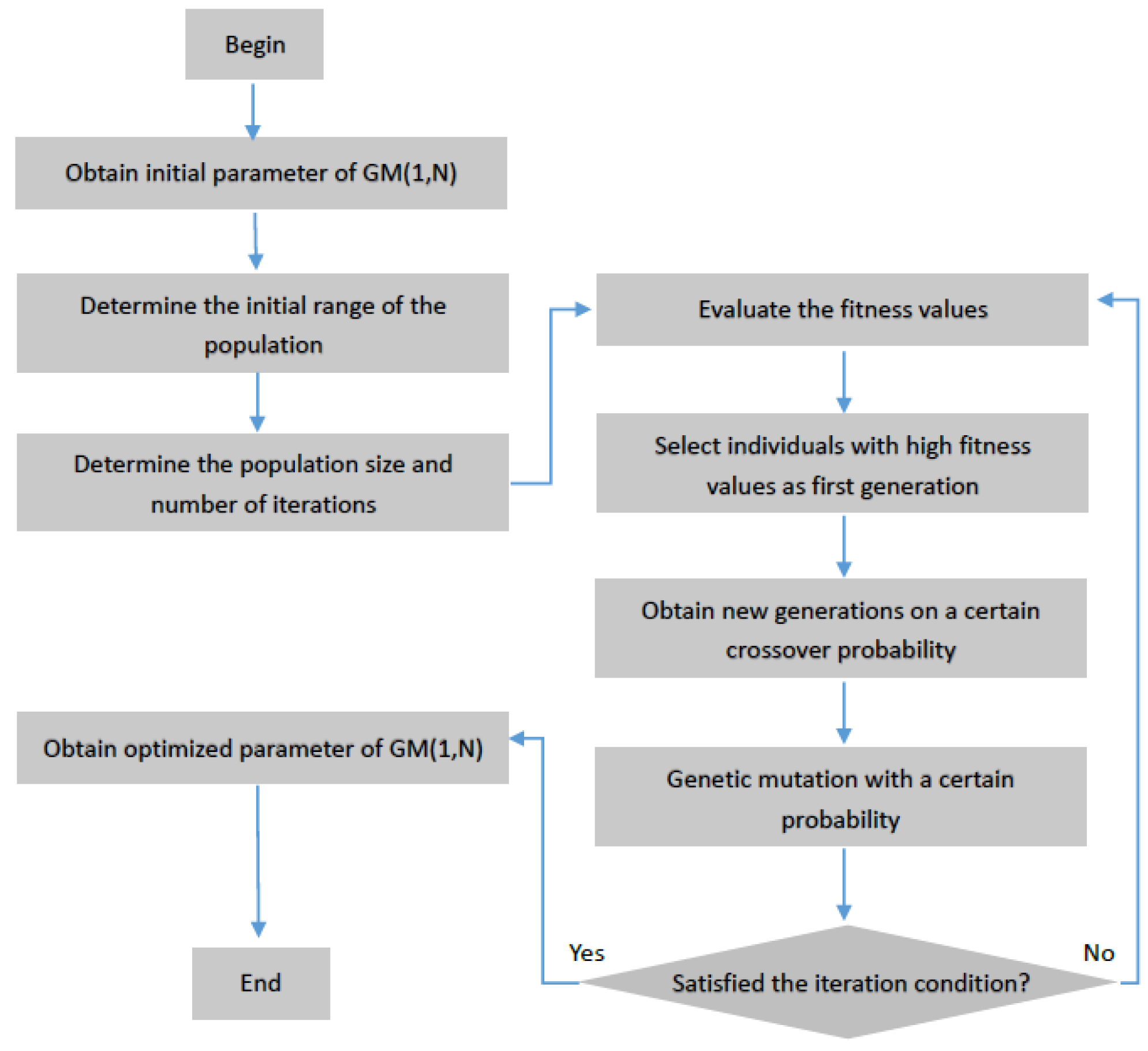
3.3. The Modelling Algorithm of GA-GM(1,N)

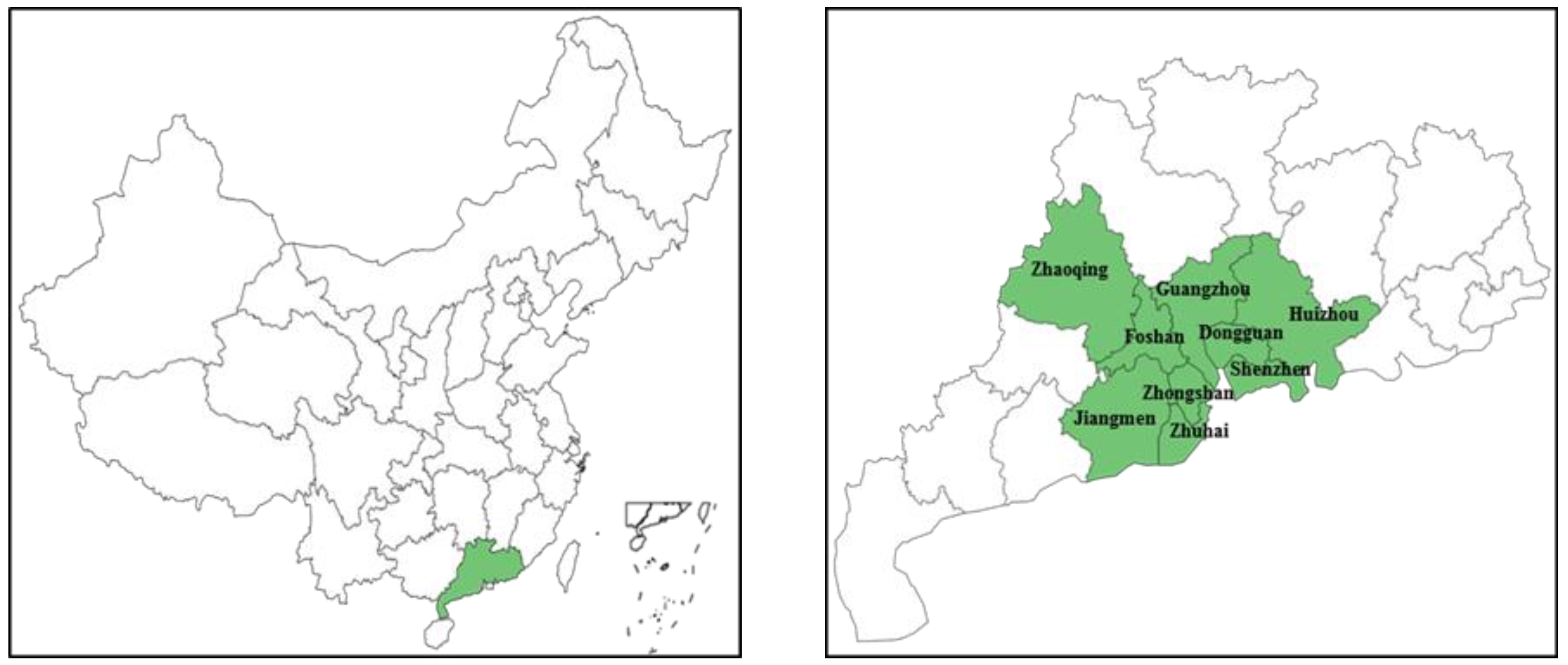
In this study, the multivariate grey model is improved using a genetic algorithm by optimizing the initial parameters to calculate optimal values. Through a number of iterations, the optimal parameters of GM(1,N) can be found. Then, the optimal GM(1,N) can be built based on optimized parameters, and the future data points can be forecast.

The basic steps of the genetic algorithm are selection, crossover and mutation [42]. The procedure of genetic algorithm is described as follows:

Step 1: Produce individuals randomly in the initial population.

Suppose that the parameters of the GM(1,N) model are recorded as S₀ = (a,b₁,b₂,…,b_n), then the initial population of the genetic algorithm can be determined, where the lower bound is S_l = (0.98a,0.98b₁,0.98b₂,…,0.98b_n) and the upper bound is S_u = (1.02a,1.02b₁,1.02b₂,…,1.02b_n).

Step 2: The fitness function is proposed to evaluate fitness value for each individual.

The fitness function can be defined as in Equation (12) [43]:

$$f_k=\frac{1}{1+\frac{1}{n}{\displaystyle \sum _{i=1}^n{\left(ob{s}_i-pr{e}_i\right)}^2}},k=1,2,\dots ,100$$

(12)

Step 3: Select the individuals based on the selection method.

Step 4: Perform crossover and mutation operation with a certain probability.

Step 5: Repeat from step 2 until the terminating condition is satisfied.

According to relevant studies on single-variable grey models optimized by a genetic algorithm [33,34], specific parameters are set as follows (

Table 1. Parameters of genetic algorithm.

Parameters	Value
Population size	100
Iteration times	1000
Crossover chance	0.7
Mutation chance	0.1

):

Using the genetic algorithm, the optimal parameters of GM(1,N) are selected with the highest fitness values. The optimization process of GA-GM(1,N) is shown in Figure 1.

4. Materials

4.1. Data and Source

As one of three economic areas in China, the Pearl River Delta, which includes nine cities (Guangzhou, Shenzhen, Zhuhai, Foshan, Huizhou, Dongguan, Zhongshan, Jiangmen and Zhaoqing) is located at Guangdong Province (Figure 2).

All the data used in this study come from Guangdong Energy Statistical Yearbook, Guangdong Statistical Yearbook and Statistical Yearbooks of the Pearl River Delta Cities. The data selected are for the years 2005 to 2015 (i.e., a total of 11 samples). The real value of GDP was adjusted to constant prices for 2005 in order to eliminate the impact of price factors.

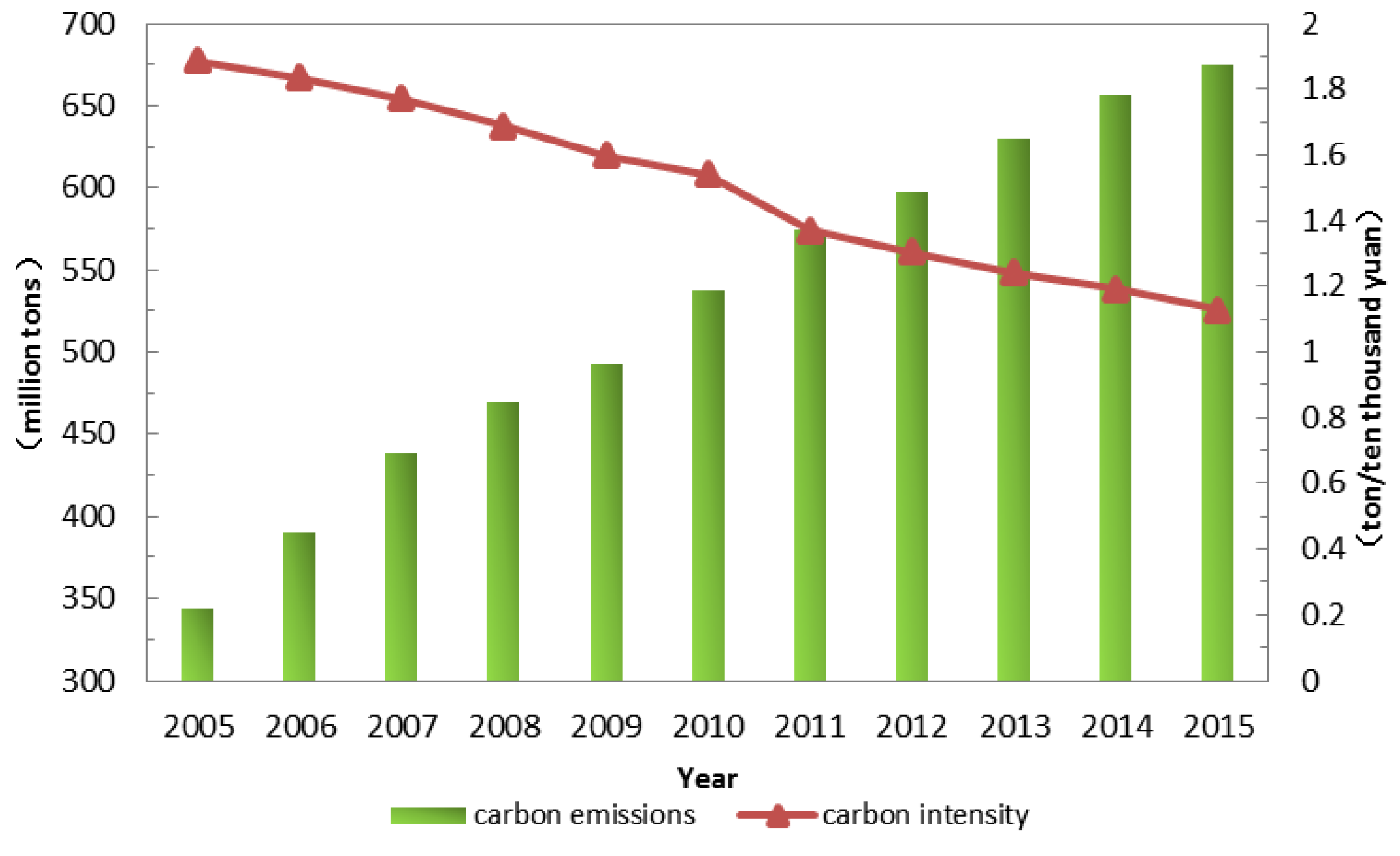
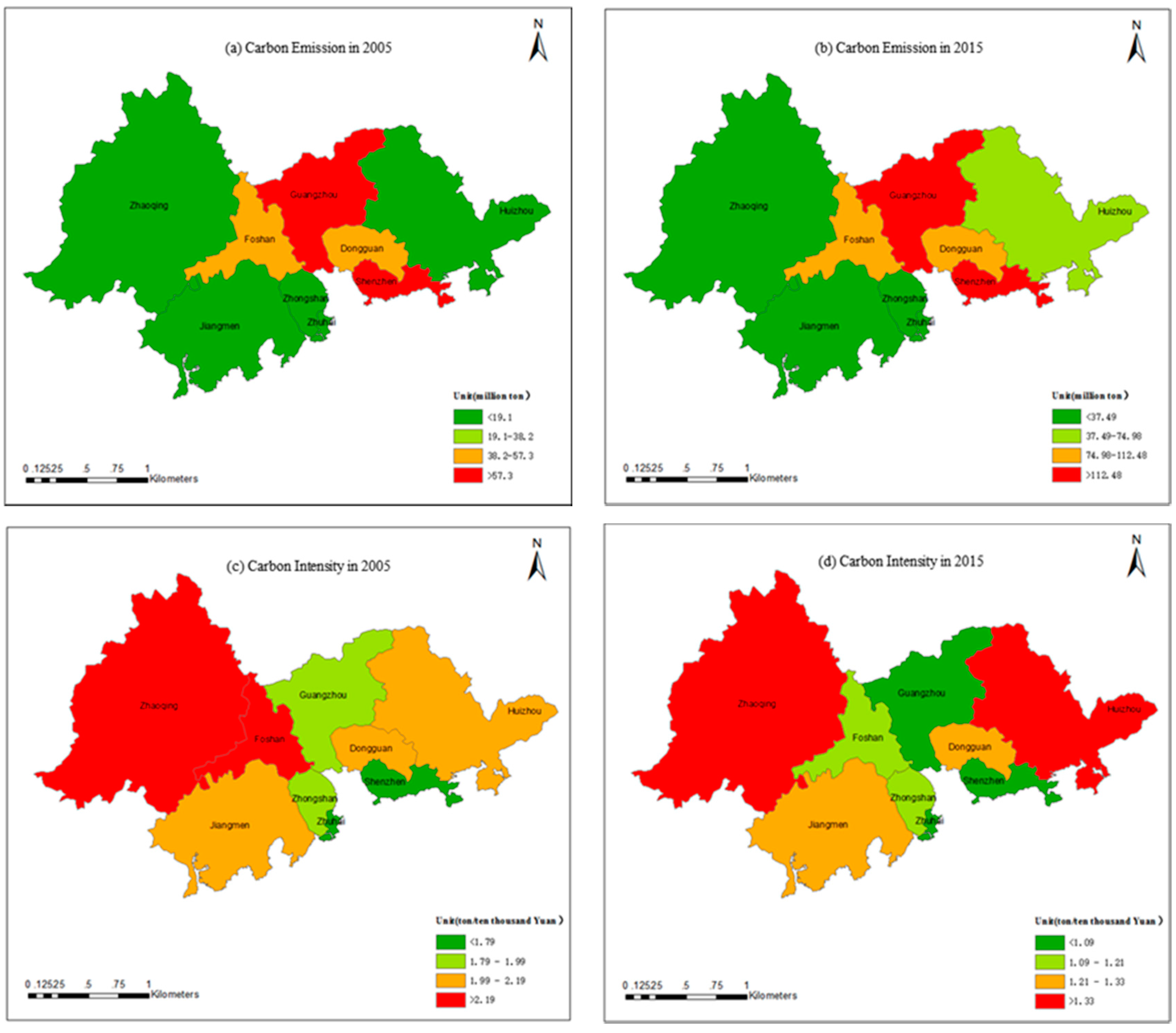
4.2. Calculation of Carbon Emissions and Carbon Intensity

Considering the absence of carbon emissions and carbon intensity data in Pearl River Delta, the relevant data were calculated using the coefficient method. The carbon emissions were calculated as follows [44]:

$$C=KE$$

(13)

where C represents the carbon emissions, K is a carbon emission coefficient and E is energy output. The coefficient K changes according to the specific regions, technical conditions and energy structures. According to the Energy Institute of China National Development and Reform Committee, the utilization rate of coal is 67%. That means 0.67 tons of carbon is converted into 2.457 tons of carbon dioxide per tce. It is assumed that the K is a constant and equal to 2.457.

Carbon intensity (CI) is the ratio of carbon output to GDP:

$$CI=\frac{C}{GDP}$$

(14)

Carbon emissions and carbon intensity of the Pearl River Delta in 2005–2015 are shown in Figure 3, with the results calculated from Equations (13) and (14).

To show the spatial distribution of carbon emissions and carbon intensity in different cities intuitively, the nine cities were divided into four types using thresholds of 0.5, 1 and 1.5 times the average carbon emission, and 0.9, 1 and 1.1 times the average carbon intensity (Figure 4). The pattern of carbon emission in 2005 is the same as that in 2015, except for Huizhou. The results show that carbon emissions are mainly concentrated in the central region of Pearl River Delta. However, the pattern of carbon intensity is the reverse of that for carbon emission. Moreover, Figure 4c,d show that carbon intensity decreased in Guangzhou and Foshan, while in Huizhou it increased.

4.3. Correlations between the Reference Sequence and the Comparison Sequences

The correlations between carbon intensity and its influencing factors are obtained based on grey relational analysis. The calculated values of grey relational coefficient are shown in

Table 2. Correlations between the reference sequence and the comparison sequences.

Region	GDP	Population	Energy Consumption	Industrial Structure
Guangzhou	0.63	0.59	0.55	0.6
Shenzhen	0.62	0.56	0.53	0.81
Zhuhai	0.65	0.56	0.57	0.53
Foshan	0.54	0.52	0.59	0.56
Huizhou	0.67	0.52	0.56	0.52
Dongguan	0.6	0.64	0.61	0.63
Zhongshan	0.65	0.63	0.58	0.66
Jiangmen	0.61	0.52	0.54	0.61
Zhaoqing	0.69	0.65	0.58	0.6
Pearl River Delta	0.62	0.51	0.54	0.57

. Grey relational coefficient is used for determining how close between the reference sequence and the comparison sequences. The larger coefficient values means that the comparison sequences are closer to the reference sequence.

With all the above absolute values, these factors are suitable to be used as dependent variables in a multivariable grey model.

4.4. Forecasting Scenarios

In order to predict the carbon intensity of each city in the Pearl River Delta from 2016 to 2020, the GM(1,N) and GA-GM(1,N) model need information about variance ratios of GDP, population, energy consumption and Industrial structure as inputs. Under The Thirteenth Five-Year Plan of Guangdong Province, the energy intensity in 2020 should be decreased by 17% from that in 2015; as yet, though, there is no target for energy consumption. Therefore, in this study, energy consumption for each city is derived from figures for GDP and energy intensity. The economic and population growth rates for each city are based on The Thirteenth Five-Year Plan and Urban Master Planning Report (

Table 3. Economic and population growth rates, 2016 to 2020 (%).

Region	GDP			Population
	LD	MD	HD
Guangzhou	7.2	7.5	7.8	3
Shenzhen	7.2	7.5	7.8	4
Zhuhai	8.7	9	9.3	2
Foshan	7.2	7.5	7.8	4
Huizhou	9.2	9.5	9.8	3
Dongguan	7.7	8	8.3	3
Zhongshan	8.5	8.5	8.5	4
Jiangmen	8.7	9	9.3	4
Zhaoqing	8.7	9	9.3	3
Pearl River Delta	7.2	7.5	7.8	3

). It is assumed that industrial structure will remain the same over the period 2011–2015. In view of actual situation of economic development, the growth rates of GDP are set to low, medium and high, represent for “Low development scenario”(LD), “Base development scenario”(BD) and “High development scenario”(HD), respectively. (Table 3).

5. Results and Discussion

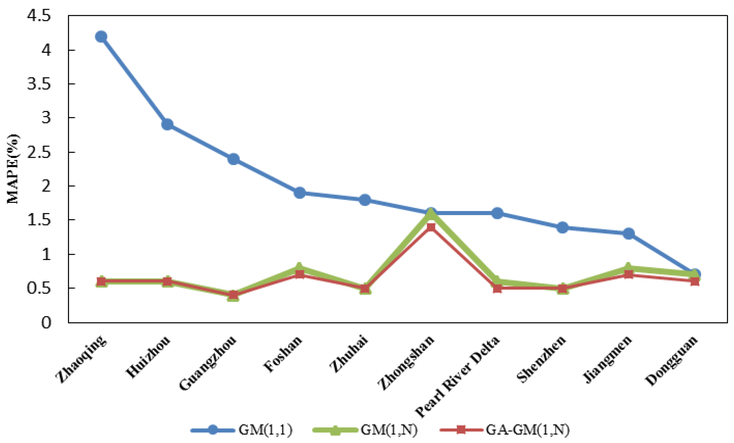
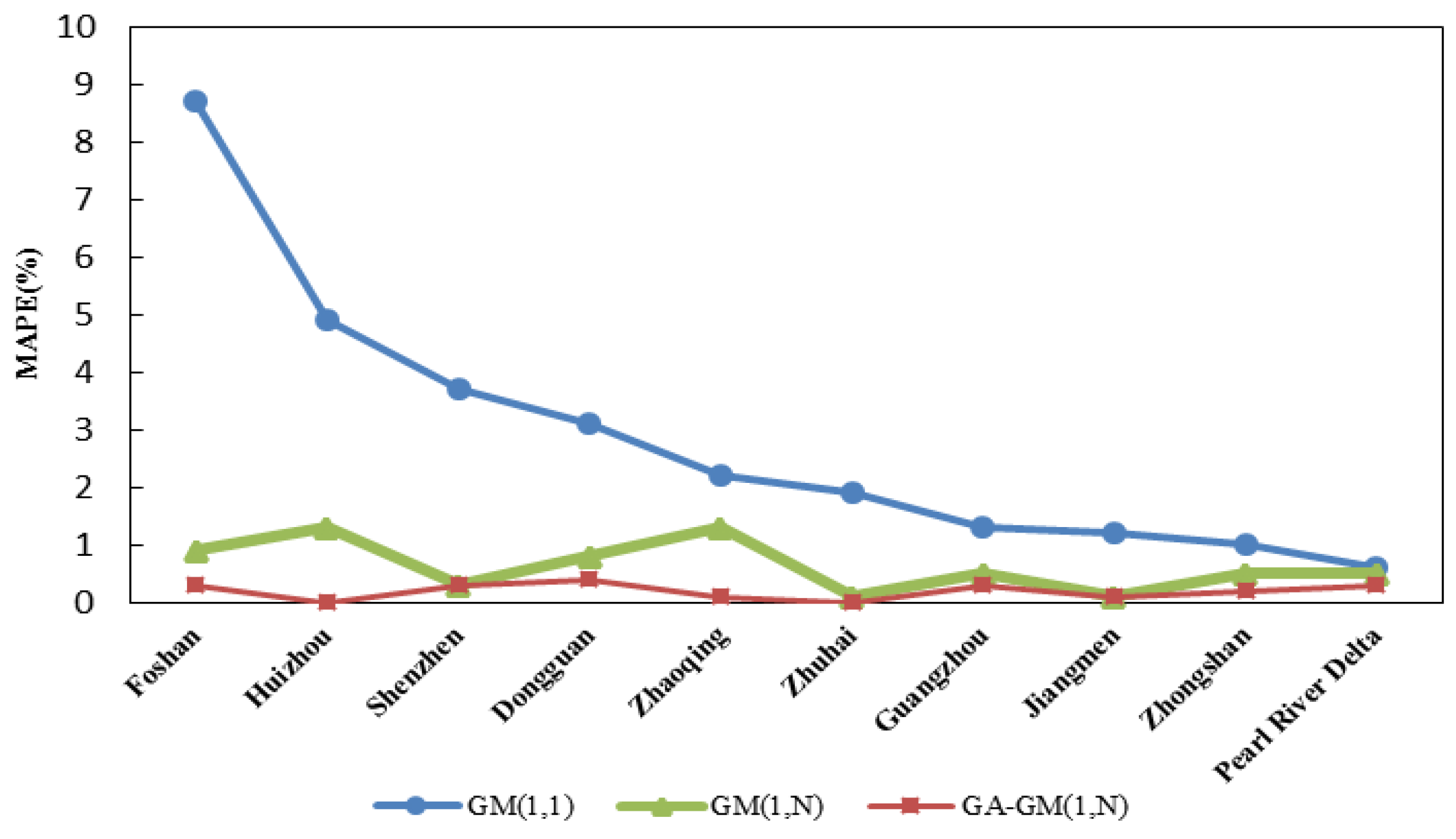
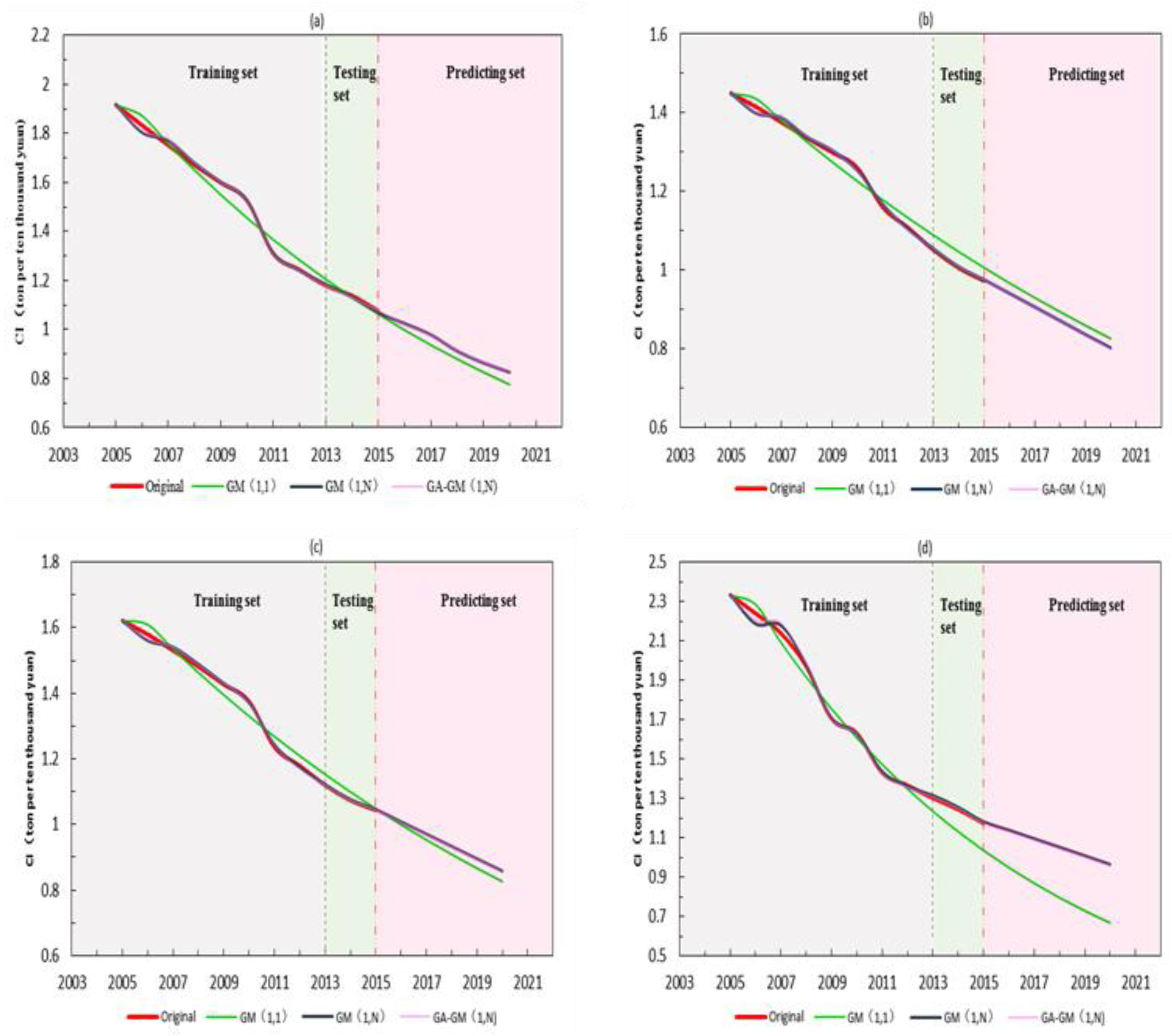
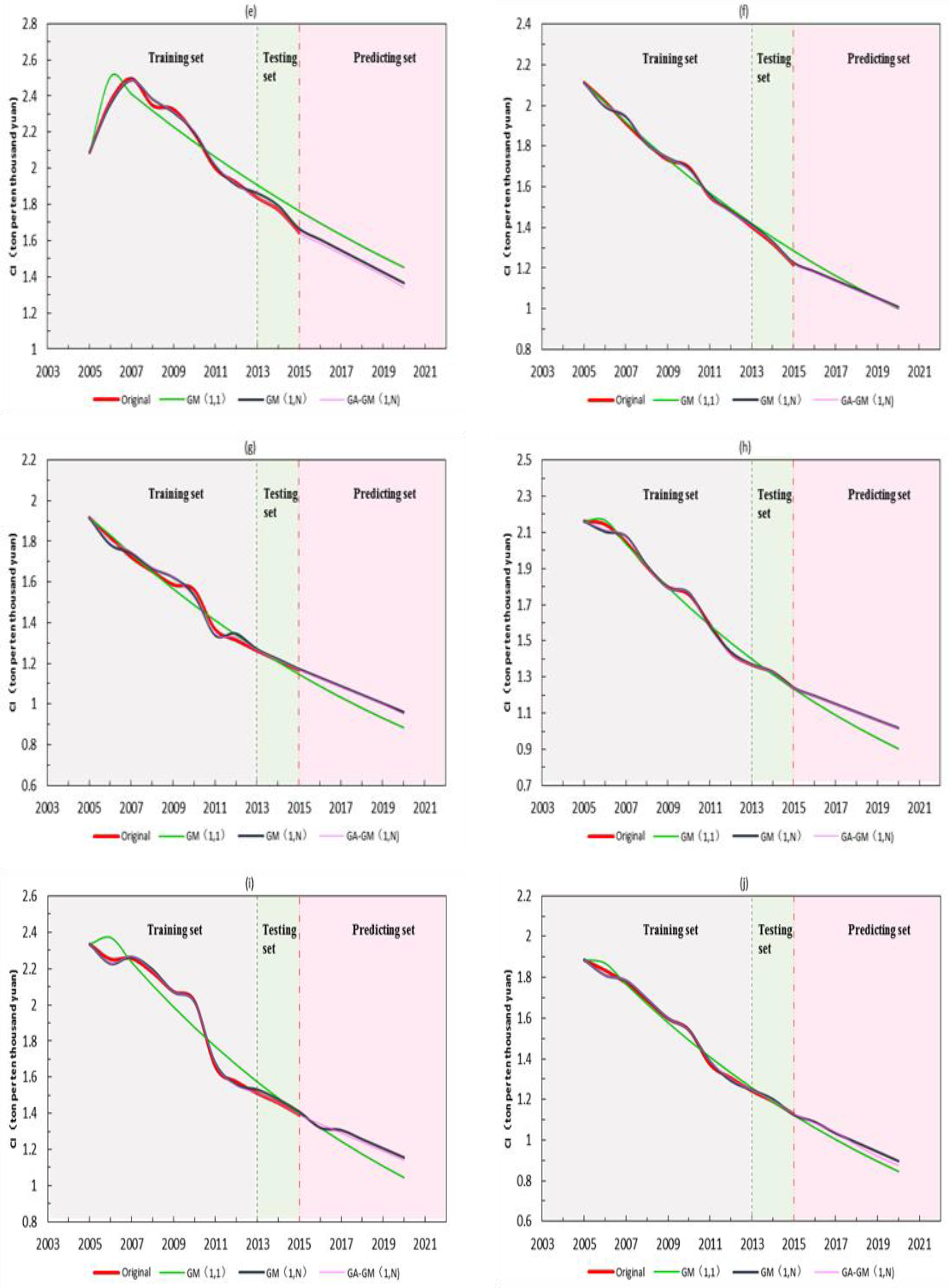
5.1. Training and Testing

As non-linear models require data for fitting, eight of the 11 samples were selected as the training datasets (2005–2012), while the remaining three datasets were used for testing (2013–2015). In line with related research on prediction [45], the mean absolute percentage error (MAPE) is was used to evaluate the forecasting performance of models GM (1,1), GM(1,N) and GA-GM(1,N) (Equation (15)). The accuracy of prediction can be considered high when MAPE is less than 10% [46]:

$$MAPE=\frac{1}{n}{\displaystyle \sum _{i=1}^n\left|\frac{ob{s}_i-pr{e}_i}{ob{s}_i}\right|}\times 100\%$$

(15)

where obs_i and pre_i are observed values and predicted values. The MAPEs of the training set are shown in Figure 5. The MAPEs are between 0.7% and 4.2% when using GM(1,1); however, these value drop to 0.4% and 1.6% when adopting GM(1,N). The prediction accuracy of the multivariable grey model is significantly improved compared with the single-variable model for all cities except Zhongshan and Dongguan. That is to say, GM(1,N) is better at predicting carbon intensity than GM(1,1). For all regions, the MAPEs are found to be lowest with model GA-GM(1,N), falling in the range 0.4% to 1.4%. Evidently, model GA-GM(1,N) improves the prediction accuracy of GM(1,N).

The MAPEs of the testing set are shown in Figure 6. The MAPEs of GM(1,N) are obviously lower than those of GM(1,1). The largest decline in MAPEs, of 7.8 percentage points, occurred in Foshan, while the value for the Pearl River Delta region as a whole was the smallest, at 0.1 percentage points.

As with the results of training set (above), the lowest prediction error was given by the GA-GM(1,N) model in all regions, ranging from 0.04 to 0.4%. GA-GM(1,N) performed excellently in forecasting the carbon intensity of Pearl River Delta as a whole, and all cities separately.

5.2. Comparative Analysis of Forecasting

The prediction results of the three methods are shown along with the original values in Figure 7. The left-hand purple area shows the results from the training set (2005–2012), while the middle green one and right-hand pink area show the results from the testing set (2013–2015) and the prediction set (2016–2020), respectively. Observed values are represented by the red lines, which consist of inflection points. However, the predicted sequences obtained by model GM(1,1) are nearly smooth descending curves. This implies that the model GM(1,1) works well when the time series demonstrates a steady growth or decline but does not perform well when the data are oscillating. GM(1,N) performed better in fitting the original data, and also produced the inflection points evident in the original data. This verifies that the grey forecasting model with multiple variables gives better forecasts than the single-variable model. After optimization using the genetic algorithm method, the accuracy of forecasting was further improved. This shows that the newly proposed genetic algorithm is an attractive and effective optimization tool for forecasting carbon intensity.

Comparing the prediction stage among three models, GM(1,1) predicts a faster decline in carbon intensity than GM(1,N) and GA-GM(1,N), except for two cities, Shenzhen and Huizhou. In addition, the rates of decline predicted by the three models are lower than the actual rates in the last five years of the original data, expect for Foshan. All three forecast models predict that the rates of decline in carbon intensity will be insufficient to meet targets.

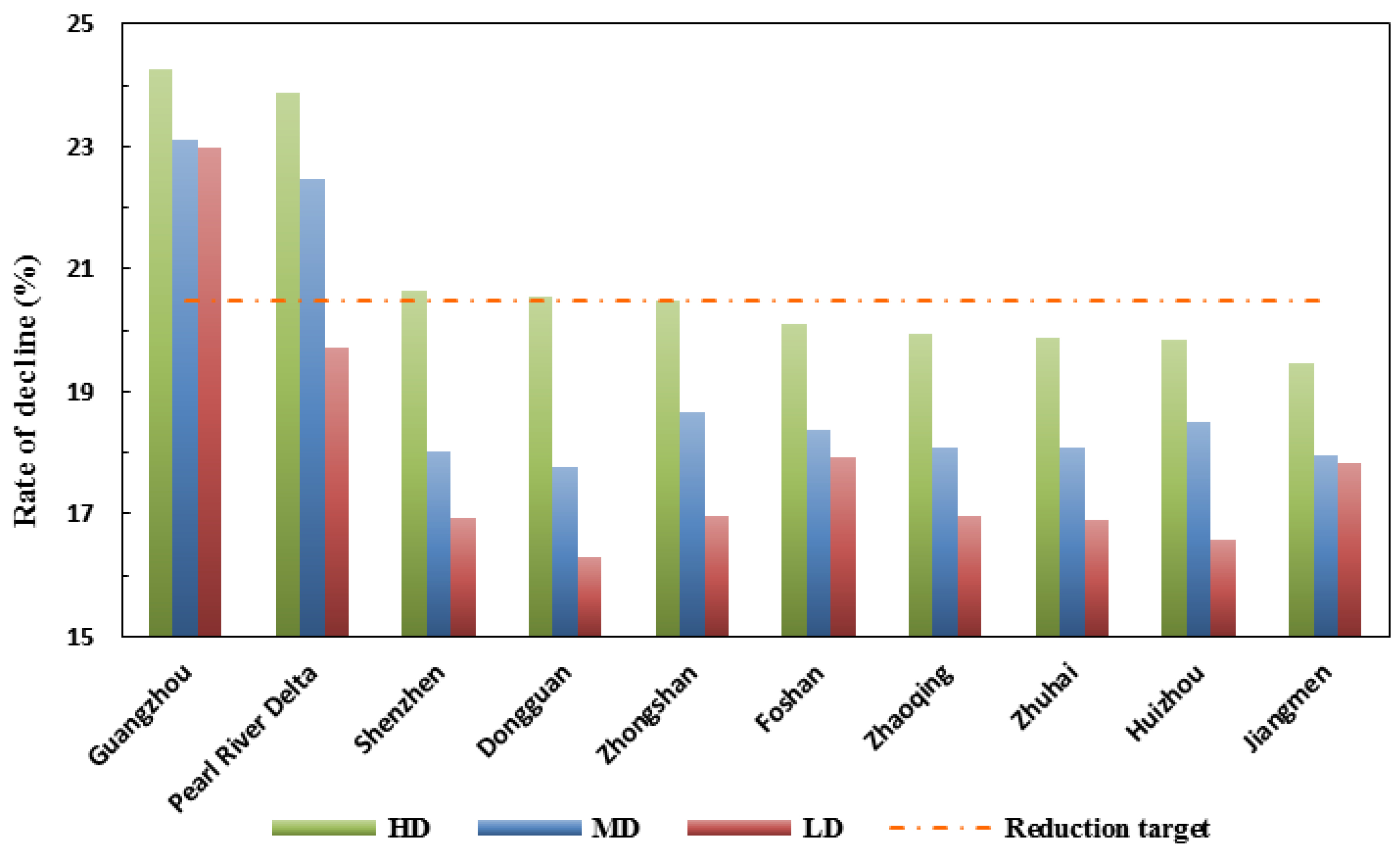
5.3. Analysis of Reduction Rate Based on Different Development Scenarios

In the previous section, the rates of decline in carbon intensity in all regions were decreasing, according to the predictions from all three models. In this section, model GA-GM(1,N)—the one with the greatest accuracy—is employed to forecast carbon intensity in 2020 under three economic development scenarios (shown in Table 3). The results are shown in Figure 8.

Comparing predicted carbon intensity in 2020 in the different economic development scenarios, it is easy to see that the higher the level of economic development is, the more likely it is that the reduction target will be achieved; the magnitude of the decline is different, though. That is to say, decreases in carbon intensity can be achieved through economic development for both Pearl River Delta and each city. There are similar conclusions from the empirical analysis of national and regional carbon intensity of China [47].

The results indicate that the growth of the economy contributes to a reduction in carbon intensity at both national level and regional level. It is generally known that carbon intensity drops when the GDP growth rate is greater than the growth rate of carbon emissions [48]. Zhao et al. [49] believe that this is because, in developed areas, better technical/technological conditions allow for greater carbon reduction.

Under the “base development scenario”, it would be difficult for any city to reach the target of 20.5%, except for Guangzhou. However, it should be noted that it could be achieved from the perspective of Pearl River Delta as a whole. This indicates that the overall objectives of the region can be achieved by particular cities taking the lead. With faster economic growth, the reduction targets will be able to be met by Shenzhen, Dongguan and Zhongshan. The GA-GM(1,N) forecast model suggests that Foshan, Zhaoqing, Zhuhai, Huizhou and Jiangmen will not be able to meet their reduction targets.

6. Conclusions

In light of climate change, as one of three major economic areas in China, carbon intensity reduction in the Pearl River Delta is of great importance. In this study, a multivariate grey model optimized by a genetic algorithm is proposed. First, the carbon emissions and carbon intensities of the nine cities in the Pearl River Delta were calculated for 2005–2015. Then carbon intensity was forecast based on variables of GDP, population, energy consumption and industrial structure. The forecasting performance of the three grey models were compared. Then, the rates of reduction in carbon intensity under different economic development scenarios were examined. From this, we draw the following conclusions:

(1)

During the period covered by the Thirteenth Five-Year Plan, all three prediction models suggest that both carbon intensity and its variation will decline. The reduction in carbon intensity will continue, but decrease.

(2)

Among the three grey models, the lowest prediction errors were given with GA-GM(1,N) at both the training and the testing stages, which indicates that the prediction accuracy of a multivariate grey model is improved by using a genetic algorithm. The newly proposed genetic algorithm is an attractive and effective optimization tool for carbon intensity forecasting.

(3)

Under all three scenarios, of the nine cities only Guangzhou could achieve its reduction target. It could serve as a reference or pattern for low-carbon development for other cities, particularly those that are likely to fail to meet their targets, such as Foshan, Zhaoqing, Zhuhai, Huizhou and Jiangmen. Due to the contribution of its low-carbon cities, Pearl River Delta could take the lead in achieving the reduction task of Guangdong Province under the “Base development scenario” and “High development scenario”.

Because it has the highest economic income and the lowest proportion of secondary industry, Guangzhou contributed a lot in achieving the reduction target of the Pearl River Delta. This has policy implications. For cities with rapid economic development, the balance between energy consumption and economic development is the key problem. More attention should be paid to technical upgrades in order to improve energy efficiency continuously. Also, the energy structure is expected to be adjusted by increasing the proportion of non-fossil fuels, such as hydropower, wind power, nuclear power and natural gas. Within secondary industry, economic growth should be focused on high value-added industries. High-energy and high-pollution enterprises should be targeted to control regional carbon emissions. In addition, other policy instruments can also be adopted, such as carbon taxes and carbon trading.

References

1. De Richter, R.K.; Ming, T.; Caillol, S.; Liu, W. Fighting global warming by GHG removal: Destroying CFCs and HCFCs in solar-wind power plant hybrids producing renewable energy with no-intermittency. Int. J. Greenh. Gas Control 2016, 49, 449–472. [Google Scholar] [CrossRef]
2. Available online:https://data.worldbank.org.cn/indicator/EN.ATM.CO2E.PP.GD?view=map (accessed on 3 November 2017).
3. Jalil, A.; Mahmud, S.F. Environment Kuznets curve for CO2, emissions: A Cointegration analysis for China. Energy Policy 2009, 37, 5167–5172. [Google Scholar] [CrossRef]
4. Liao, F.H.F.; Wei, Y.D. Dynamics, space, and regional inequality in provincial China: A case study of Guangdong province. Appl. Geogr. 2012, 35, 71–83. [Google Scholar] [CrossRef]
5. Available online:http://www.gdstats.gov.cn/tjnj/2016/directory/content.html?02-15 (accessed on 3 November 2017).
6. Yi, W.J.; Zou, L.L.; Jie, G.; Kai, W.; Wei, Y.M. How can China reach its CO2, intensity reduction targets by 2020? A regional allocation based on equity and development. Energy Policy 2011, 39, 2407–2415. [Google Scholar] [CrossRef]
7. Clough, S. Achieving CO2, reductions in Colombia: Effects of carbon taxes and abatement targets. Energy Econ. 2016, 56, 575–586. [Google Scholar]
8. Qiang, D.; Ning, W.; Lei, C. Forecasting China’s per capita carbon emissions under a new three-step economic development strategy. J. Resour. Ecol. 2015, 6, 318–323. [Google Scholar] [CrossRef]
9. Wu, Q.; Peng, C. Scenario analysis of carbon emissions of China’s electric power industry up to 2030. Energies 2016, 9, 988. [Google Scholar] [CrossRef]
10. Sun, W.; Wang, C.; Zhang, C. Factor analysis and forecasting of CO2 emissions in Hebei, using extreme learning machine based on particle swarm optimization. J. Clean. Prod. 2017, 162, 1095–1101. [Google Scholar] [CrossRef]
11. Zhu, B.; Wang, K.; Chevallier, J.; Wang, P.; Wei, Y.M. Can China achieve its carbon intensity target by 2020 while sustaining economic growth? Ecol. Econ. 2015, 119, 209–216. [Google Scholar] [CrossRef]
12. Xiao, B.; Niu, D.; Guo, X. Can China achieve its 2020 carbon intensity target? A scenario analysis based on system dynamics approach. Ecol. Indic. 2016, 71, 99–112. [Google Scholar] [CrossRef]
13. Wang, R.; Liu, W.; Xiao, L.; Jian, L.; Kao, W. Path towards achieving of China’s 2020 carbon emission reduction target—A discussion of low-carbon energy policies at province level. Energy Policy 2011, 39, 2740–2747. [Google Scholar] [CrossRef]
14. Yu, B.; Li, X.; Qiao, Y.; Shi, L. Low-carbon transition of iron and steel industry in China: Carbon intensity, economic growth and policy intervention. J. Environ. Sci. 2015, 28, 137–147. [Google Scholar] [CrossRef] [PubMed]
15. Cansino, J.M.; Román, R.; Rueda-Cantuche, J.M. Will China comply with its 2020 carbon intensity commitment? Environ. Sci. Policy 2015, 47, 108–117. [Google Scholar] [CrossRef]
16. Kayacan, E.; Ulutas, B.; Kaynak, O. Grey system theory-based models in time series prediction. Expert Syst. Appl. 2010, 37, 1784–1789. [Google Scholar] [CrossRef]
17. Zhou, P.; Ang, B.W.; Poh, K.L. A trigonometric grey prediction approach to forecasting electricity demand. Energy 2006, 31, 2839–2847. [Google Scholar] [CrossRef]
18. Zhao, Z.; Wang, J.; Zhao, J.; Su, Z. Using a grey model optimized by differential evolution algorithm to forecast the per capita annual net income of rural households in China. Omega 2012, 40, 525–532. [Google Scholar] [CrossRef]
19. Wang, J.; Yan, R.; Hollister, K.; Zhu, D. A historic review of management science research in China. Omega 2008, 36, 919–932. [Google Scholar] [CrossRef]
20. Ding, S.; Dang, Y.-G.; Li, X.-M.; Wang, J.-J.; Zhao, K. Forecasting Chinese CO2, emissions from fuel combustion using a novel grey multivariable model. J. Clean. Prod. 2017, 162, 1527–1538. [Google Scholar] [CrossRef]
21. Akay, D.; Atak, M. Grey prediction with rolling mechanism for electricity demand forecasting of Turkey. Energy 2007, 32, 1670–1675. [Google Scholar] [CrossRef]
22. Liu, X.; Cuartas, B.M.; Muñiz, A.S.G. A grey neural network and input–output combined forecasting model. Primary energy consumption forecasts in Spanish economic sectors. Energy 2016, 115, 1042–1054. [Google Scholar] [CrossRef]
23. Deng, J.L. Grey Prediction and Decision; HUST Press: Wuhan, China, 2002. (In Chinese) [Google Scholar]
24. Guo, H.; Xiao, X.; Forrest, J. A research on a comprehensive adaptive grey prediction model CAGM(1,n). Appl. Math. Comput. 2013, 225, 216–227. [Google Scholar] [CrossRef]
25. Wang, Z.X.; Hao, P. An improved grey multivariable model for predicting industrial energy consumption in China. Appl. Math. Model. 2016, 40, 5745–5758. [Google Scholar] [CrossRef]
26. Canyurt, O.E.; Ozturk, H.K. Application of genetic algorithm (GA) technique on demand estimation of fossil fuels in Turkey. Energy Policy 2008, 36, 2562–2569. [Google Scholar] [CrossRef]
27. Hong, W.C.; Dong, Y.; Zhang, W.Y.; Chen, L.Y.; Panigrahi, B.K. Cyclic electric load forecasting by seasonal with chaotic genetic algorithm. Int. J. Electr. Power Energy Syst. 2013, 44, 604–614. [Google Scholar] [CrossRef]
28. Holland, J.H. Adaptation in Natural and Artificial Systems; MIT Press: London, UK, 1992. [Google Scholar]
29. Zhang, K.; Du, H.; Feldman, M.W. Maximizing influence in a social network: Improved results using a genetic algorithm. Phys. A Stat. Mech. Appl. 2017, 478, 20–30. [Google Scholar] [CrossRef]
30. Gao, M.; Shi, G.; Li, W.; Wang, Y.; Liu, D. An improved genetic algorithm for island route planning. Procedia Eng. 2017, 174, 433–441. [Google Scholar] [CrossRef]
31. Zamzamian, S.M.; Hosseini, S.A.; Samadfam, M. Optimization of the Marinelli beaker dimensions using genetic algorithm. J. Environ. Radioact. 2017, 172, 81–88. [Google Scholar] [CrossRef] [PubMed]
32. Benet, C.H.; Kassler, A.; Zola, E. Predicting expected TCP throughput using genetic algorithm. Comput. Netw. 2016, 108, 307–322. [Google Scholar] [CrossRef]
33. Yuan, J.L.; Li, X.Y.; Zhong, L. Optimized Grey RBF Prediction Model Based on Genetic Algorithm. In Proceedings of the International Conference on Computer Science and Software Engineering, Wuhan, China, 2008; pp. 74–77. [Google Scholar]
34. Ou, S.L. Forecasting agricultural output with an improved grey forecasting model based on the genetic algorithm. Comput. Electron. Agric. 2012, 85, 33–39. [Google Scholar] [CrossRef]
35. Choi, J.W.; Lee, H.; Lee, J.C.; Lee, S.; Kim, Y.S.; Yoon, H.; Kim, H.C. Application of genetic algorithm for hemodialysis schedule optimization. Comput. Methods Programs Biomed. 2017, 145, 35–43. [Google Scholar] [CrossRef] [PubMed]
36. Deng, J.L. Control problems of grey systems. Syst. Control Lett. 1982, 1, 288–294. (In Chinese) [Google Scholar]
37. Bhattacharyya, S.C.; Ussanarassamee, A. Decomposition of energy and CO2, intensities of Thai industry between 1981 and 2000. Energy Econ. 2004, 26, 765–781. [Google Scholar] [CrossRef]
38. Li, J.; Lin, B. Inter-factor/inter-fuel substitution, carbon intensity, and energy-related CO2, reduction: Empirical evidence from China. Energy Econ. 2016, 56, 483–494. [Google Scholar] [CrossRef]
39. Zhang, W.; Li, K.; Zhou, D.; Zhang, W.; Gao, H. Decomposition of intensity of energy-related CO2, emission in Chinese provinces using the LMDI method. Energy Policy 2016, 92, 369–381. [Google Scholar] [CrossRef]
40. Kadier, A.; Abdeshahian, P.; Simayi, Y.; Ismail, M.; Hamid, A.A.; Kalil, M.S. Grey relational analysis for comparative assessment of different cathode materials in microbial electrolysis cells. Energy 2015, 90, 1556–1562. [Google Scholar] [CrossRef]
41. Yuan, Z.; Wu, L.; Yuan, Z.; Li, H. Shape optimization of welded plate heat exchangers based on grey correlation theory. Appl. Therm. Eng. 2017, 123, 761–769. [Google Scholar]
42. Kolonko, M. A generalized crossover operation for genetic algorithms. Complex Syst. 1995, 9, 177–191. [Google Scholar]
43. Junior, A.R.L. A study for multi-objective fitness function for time series forecasting with intelligent techniques. In Proceedings of the Conference Companion on Genetic and Evolutionary Computation, Atlanta, GA, USA, 12–16 July 2008; ACM: New York, NY, USA, 2008; pp. 1843–1846. [Google Scholar]
44. Liao, Z.; Zhu, X.; Shi, J. Case study on initial allocation of Shanghai carbon emission trading based on Shapley value. J. Clean. Prod. 2015, 103, 338–344. [Google Scholar] [CrossRef]
45. Pao, H.T.; Fu, H.C.; Tseng, C.L. Forecasting of CO2, emissions, energy consumption and economic growth in China using an improved grey model. Energy 2012, 40, 400–409. [Google Scholar] [CrossRef]
46. Lewis, C.D. Industrial and Business Forecasting Methods: A Practical Guide to Exponential Smoothing and Curve Fitting; Butterworth Scientific, Heinemann: London, UK, 1982. [Google Scholar]
47. Wang, Z.; Zhang, B.; Liu, T. Empirical analysis on the factors influencing national and regional carbon intensity in China. Renew. Sustain. Energy Rev. 2016, 55, 34–42. [Google Scholar] [CrossRef]
48. Yu, S.; Zhang, J.; Zheng, S.; Sun, H. Provincial carbon intensity abatement potential estimation in China: A PSO–GA-optimized multi-factor environmental learning curve method. Energy Policy 2015, 77, 46–55. [Google Scholar] [CrossRef]
49. Zhao, X.; Zhang, X.; Li, N.; Shao, S.; Geng, Y. Decoupling economic growth from carbon dioxide emissions in China: A sectoral factor decomposition analysis. J. Clean. Prod. 2017, 142, 3500–3516. [Google Scholar] [CrossRef]
Figure 1. The flow chart of the GM(1,N) model optimized using a genetic algorithm.
Energies 11 00091 g001
Figure 2. The map of Guangdong Province and Pearl River Delta.
Energies 11 00091 g002
Figure 3. Carbon emissions and carbon intensity of the Pearl River Delta from 2005 to 2015.
Energies 11 00091 g003
Figure 4. Carbon emissions and carbon intensity of the Pearl River Delta in 2005 and 2015.
Energies 11 00091 g004
Figure 5. MAPEs of the training set using different models.
Energies 11 00091 g005
Figure 6. MAPEs of the testing set using different models.
Energies 11 00091 g006
Figure 7. Observed values and Predicted values of Carbon Intensity in Pearl River Delta (2005–2020). ((a) Guangzhou; (b) Shenzhen; (c) Foshan; (d) Zhuhai; (e) Huizhou; (f) Dongguan; (g) Zhongshan; (h) Jiangmen; (i) Zhaoqing; (j) Pearl River Delta).
Energies 11 00091 g007aEnergies 11 00091 g007b
Figure 8. Rates of decline in carbon intensity in three economic development scenarios.
Energies 11 00091 g008