Abstract
As an imperative part of smart grids (SG) technology, the optimal operation of active distribution networks (ADNs) is critical to the best utilization of renewable energy and minimization of network power losses. However, the increasing penetration of distributed renewable energy sources with uncertain power generation and growing demands for higher quality power distribution are turning the optimal operation scheduling of ADN into complex and global optimization problems with non-unimodal, discontinuous and computation intensive objective functions that are difficult to solve, constituting a critical obstacle to the further advance of SG and ADN technology. In this work, power generation from renewable energy sources and network load demands are estimated using probability distribution models to capture the variation trends of load fluctuation, solar radiation and wind speed, and probability scenario generation and reduction methods are introduced to capture uncertainties and to reduce computation. The Open Distribution System Simulator (OpenDSS) is used in modeling the ADNs to support quick changes to network designs and configurations. The optimal operation of the ADN, is achieved by minimizing both network voltage deviation and power loss under the probability-based varying power supplies and loads. In solving the computation intensive ADN operation scheduling optimization problem, several novel metamodel-based global optimization (MBGO) methods have been introduced and applied. A comparative study has been carried out to compare the conventional metaheuristic global optimization (GO) and MBGO methods to better understand their advantages, drawbacks and limitations, and to provide guidelines for subsequent ADN and smart grid scheduling optimizations. Simulation studies have been carried out on the modified IEEE 13, 33 and 123 node networks to represent ADN test cases. The MBGO methods were found to be more suitable for small- and medium-scale ADN optimal operation scheduling problems, while the metaheuristic GO algorithms are more effective in the optimal operation scheduling of large-scale ADNs with relatively straightforward objective functions that require limited computational time. This research provides solution for ADN optimal operations, and forms the foundation for ADN design optimization.
1. Introduction
With the rapid development of distributed generation (DG) technology, energy storage system (ESS) equipment, power distribution networks are being transformed from traditional passive load distribution systems into intelligent active distribution networks (ADNs) [1]. Future distribution networks will consist of various energy sources, serving a variety of functions of an integrated energy system. Besides that, the continued improvements and wide applications of distribution automation, data acquisition, and data transmission technologies are rapidly improving the observability and controllability of the distribution power grid, which enables the active control of the network for optimal operation. The ability to actively control the operations of DGs and ESSs in the distribution network further demands the optimal control of the grid operation to reach the full energy efficiency potential and to best utilize the available renewable energy resources in the distribution network.
The optimal operation of the active power distribution network is essentially an optimal power flow (OPF) problem, and considerable research efforts have been devoted to this area with similar optimization problem formulation and two different types of solution methods, conventional optimization methods and stochastic/metaheuristic global optimization methods, depending upon the complexity of the formulation [2]. The conventional optimization solution approach uses traditional optimization methods, including Non-Linear Programming (NLP) [3], Quadratic Programming (QP) [4], Linear Programming (LP) [5], Gradient Method, Newton Method, and Interior Point Method (IPM) to solve the optimal operation scheduling problem. These methods are efficient and effective for the OPF problems of conventional power networks due to the quadratic form of the network power flow objective function model. In many cases, the close-form solution of the network flow characteristics can be derived. However, a number of factors made this conventional approach no longer directly applicable: (a) with the additions of local renewable energy sources, such as wind and solar power generation units and ESS to the network, the more complex models for capturing the time-variant, discontinuous and uncertain behaviors of these new network elements, as well as the introduction of additional control variables have changed the unimodal and continuity nature of the optimization objective functions of the OPF problem; (b) considering and modeling embedded local sub-network in a black-box form network simulation software turns the optimization objective function more complex and ill-shaped; (c) additional network composition and operation considerations lead to the inclusion of non-continuous design variables; and (d) inclusions of more complex networks and network components result in more complex operation constraints to the optimization with non-convex feasible region. The conventional optimization methods cannot deal with these issues and ensure convergence to the global optimum of these complex network operation schedule optimization problems.
Due to the inherent limitations of the classical “local optimization methods” and the advances in computation technology, the interest in using advanced population-based evolutionary global optimization methods to solve network optimal scheduling problems has rapidly grown during the recent decades. The population-based global optimization methods use the random transition rules rather than deterministic ones to identify the global optimum through intensive computation. These algorithms do not directly use the derivative information of the objective function during the search, illustrating high ability to locate the global optimum and to cope with large-scaled non-linear problems. Widely-used population-based global optimization methods include differential evolution (DE) [6,7], particle swarm optimization (PSO) [7], genetic algorithm (GA) [8], evolutionary programming (EP) [9,10], simulated annealing (SA) [11], gravitational search algorithm (GSA) [12,13], Tabu search algorithm (TS) [14], artificial bee colony algorithm (ABC) [15], modified imperialist competitive algorithm (MOMICA) [16], and black hole optimization algorithm. These global optimization search methods are capable of solving complex global optimization problems with mixed continuous and discrete variables, and discontinuous objective function. Meanwhile, these techniques also require extensive computation in evaluating the objective and constraint functions to obtain a very large number of sample points during their stochastic search process to ensure convergence to the global optimum and robustness. These shared characteristics makes them less applicable or attractive for applications in which the objective and constraint functions of the optimization are in implicit form through computational demanding numerical simulations—the so-called computational expensive “black-box function” optimization problem (CE-BOP) [17]. The mounting computational time resulted from tens of thousands of lengthy simulations make the optimization infeasible. If the number of black-box objective function evaluation is limited, the search will likely lead to questionable results.
On the other hand, the use of a generic ADN performance modeling tool for automatic and quick generation of the optimal operation schedule for a given ADN is essential. Use network performance modeling and simulation tool, such as the Open Distribution System Simulator (OpenDSS) [18], allows quick changes to the network design and its model for dynamic operation optimization and for the design optimization of the ADN with different network configurations. Firstly, the automatic and quick generation of optimal operation schedule for a given ADN based on the modeling tool’s accurate prediction of network performance is needed for the real-time optimal operation and control of the ADN. Secondly, the generation of the optimal operation schedule for ADN using the modeling tool’s accurate network performance prediction is also needed indirectly for evaluating various ADN architecture and component sizes in the optimal design of the ADN, since all different architecture and component size designs can only be compared under their optimal operations. The combination of operation and design optimizations will ensure efficient utilization of available renewable energy sources and high efficiency of the distribution networks, while the integrated ADN performance simulation and quick global optimization software tool serve as the foundation for both.
Over the last decade, many effective search methods for solving the expensive black-box optimization problems have been introduced, including the “Divide-the-Best” algorithms [19] and the efficient diagonal partition strategy [20] which partitions the search hyperinterval into smaller hyperintervals and only evaluates the objective function at the two vertices of the main diagonal of the generated hyperintervals, to effectively avoid the unnecessary ponderous simulations. Another type of effective solution method is the surrogate or metamodel-based global optimization (MBGO) search techniques, which have been introduced and investigated by many researchers, including the authors’ group [21]. The approach uses limited “expensive” sample data points from the original, computationally expensive optimization model to introduce a surrogate model, or metamodel, such as Kriging [22] and radial basis functions (RBF) [23], and to effectively use the “cheaper” sample points from the metamodel to speed up the search of the global optimum with much reduced number of original model evaluations and computational time. Several reviews have systematically presented the advantages of these algorithms [21,24,25,26]. The newly introduced algorithms have been compared with other existing GO techniques using about a dozen of standard benchmarks optimization problems to study their capability to accurately locate the global optimum, search efficiency and computation time. Haftka, Villanueva and Chaudhuri surveyed surrogate-based global optimization algorithms with adaptive samplers that employ Gaussian Process or Kriging surrogates with a focus on how different algorithms balance exploration and exploitation, and the advantage of surrogate assisted parallel evolutionary algorithms [27]. These benchmark problems consist of a large set of objective functions of a wide variety of types, such as unimodal, multimodal, continues, discontinues, discrete, constrained, unconstrained and high dimensional, with over a hundred different benchmark test functions. Although there is no general agreement on any set of functions that can be used to validate a global optimization algorithm, these benchmark problems allow a better understanding on the comparative performance of various optimization algorithms. Further development of representative global design optimization test cases is imperative to provide effective measure and verification on the capability of new global optimization algorithm, and to guide further research.
In this work, an ADN operation schedule optimization model considering the uncertainties of both distributed generations and loads has been formulated, and the new probability-based scenario generation and reduction methods have been introduced to model and handle the uncertainties associated with the distributed generations and loads. To solve the formulated ADN operation optimization problems with single and multi-objective functions effectively, a number of novel MBGO methods, including the Space Exploration and Region Elimination (SEUMRE) algorithm, the Hybrid and Adaptive Meta-model-based (HAM) method, the Mode Pursuing Sampling (MPS) method, and the Multi-Start Space Reduction (MSSR) surrogate-based search algorithm have been introduced and applied. The IEEE 13 node, 33 node and 123 node network models have been modified to form our ADN system test cases. The computational efficiency and the global convergence of these MBGO methods are analyzed and discussed in details in comparison with the traditional population-based optimization methods. The robustness and efficiency of these MBGO methods are summarized, and the suitability of each of these optimization methods is discussed.
The rest of this paper is organized as follows: Section 2 describes the uncertainty model of distributed generations and loads. The ADN optimal operation problem considering the uncertainties of both distributed generations and loads is formulated in Section 3. The MBGO solution methods and the operation optimization procedure are described in detail in Section 4. Simulation results are presented in Section 5 to illustrate the computational efficiency and global convergence capability of the MBGO search methods. Finally, conclusions of this study are given in Section 6.
2. Uncertainty Modeling of Distributed Generations and Loads
The distributed renewable energy sources and loads in an active distribution network are associated with considerable uncertainties. To ensure the optimal operation of the ADN, these uncertainties need to be captured and model properly. In this work, power generation from renewable energy sources and network load demands are estimated using probability distribution models to capture the variation trends of load fluctuation, solar radiation and wind speed. The method of probability-based scenarios is used to represent the uncertainties of DGs and loads.
2.1. Wind Power
Wind speed prediction is the key to the operational scheduling of wind turbine generator system. Extensive researches have been investigated in developing various wind speed forecasting models. The two parameters Weibull distribution model in a simple form has been recognized to fit well with actual wind velocity distribution [28], and generally considered as most applicable. With the statistical wind speed probability density function, the model is expressed as follows:
where, is the wind speed, and are the two Weibull distribution parameters, is the shape parameter (), and is the scale parameter (). and can be obtained by the mean value and standard deviation of wind speed over the observed time as follows:
where, and are the mean value and standard deviation of wind speed respectively, is the Gamma function.
The wind power generation is then approximated by cut-in wind speed , cut-out wind speed , rated wind speed , and rated wind power generation as follows:
where, , and are curve fitting parameters of the wind turbine.
2.2. Photovoltaic Power
The photovoltaic (PV) output power is closely related to the intensity of solar radiation and ambient temperature. According to statistics, the intensity of the solar radiation can be approximately represented as a Beta distribution over a certain period of time [29], and its probability density function can be expressed as:
where, is the Gamma function, and refer to the actual illumination intensity and the maximum illumination intensity during a period of time, and are the shape parameters for the Beta distribution, which can be obtained by average illumination intensity and standard deviation of this period of time as follows:
where, and are the mean value and standard deviation of illumination intensity, respectively.
The actual output power of PV can be forecasted by comparing with the sunlight intensity, environmental temperature, and output power under standard conditions, as expressed in Equation (8):
where, the operating parameters with the subscript stc have values under standard testing conditions, ( = 1 kW/m2, and = 25 °C); is the power temperature coefficient; and is the battery surface temperature, which is a function of environmental temperature, , and radiation intensity at the operating point, :
2.3. Load Fluctuation
Extensive works have been done on the analysis of load fluctuation characteristics such as [30,31], the existing research studies have shown that the fluctuation characteristics of load are similar to normal distribution. Probability of requiring load demands can be approximately represented as follows:
where, and are the mean value and standard deviation of load demand based on the observed value, respectively.
3. Formulation of the ADN Optimal Operation Problem
3.1. Scenario Generation
To address the uncertainties of the DGs and loads in the optimization operation of ADN, the method of probability scenarios is introduced, which actually includes the probability scenario generation and scenario reduction.
Considering the multidimensional, random variation of DGs and loads, the multidimensional sampling theory is needed for multidimensional hierarchical sampling. The Latin hypercube sampling (LHS) method, an effective multidimensional hierarchical sampling method that reflects the overall distribution of random variables, ensuring that all sampling regions can be covered by the sampling points [32], is used in this work for DGs and loads uncertainty sampling to generate different probability scenarios, the detailed sampling method is as follows:
- (1)
- For any random variable , the probability of the vertical axis of the cumulative probability distribution curve of is divided into intervals, and a value is randomly extracted in each interval:
- (2)
- For the k-th sample of the random variable , the corresponding cumulative distribution probability (CDF) is:where, subject to uniform distribution. By calculating the inverse function of the cumulative distribution function , the first sample value of random variable can be obtained:
- (3)
- After the sampling is completed, the sampling values of each random variable are arranged in a column of the matrix to form a sampling matrix. The Gram-Schmidt sequence orthogonalization method is used to sort the matrix [33], and the correlation of each column is minimized by iterative calculation. Therefore, sampling scenarios are formed.
3.2. Scenario Reduction
According to the principle of LHS in Section 3.1, the larger the sampling scale is, the higher accuracy can be obtained. However, large sampling scale will also lead to heavier computational burden and reduced computational efficiency. To reduce the amount of computation and also retain the characteristics of the original scene as much as possible, similar scenarios are thus merged using the scenario reduction technique. The Synchronous Back to Generation Reduction (SBR) technique [34,35] is used here to reduce the number of scenarios and to determine the corresponding scenario probability.
Assuming that there exist N scenarios in the initial scenario set, the probability of each scenario generated by LHS is thus . Defining the 2 norms of the scenario vector as the probability distance between different scenarios, and arranging them in a descending order. By defining the final scenario number as , as the set of deleted scenarios, which is empty initially, the main steps of the scenario reduction algorithm include:
- (1)
- Calculate the probability distance between scenario and . , .
- (2)
- For each scenario , find the scenario with the shortest distance, , .
- (3)
- If the probability of scenario is , calculate and determining the scenario to be deleted by formula .
- (4)
- Corrected scenario set and the set of deleted scenarios and its associated probabilities by , , .
- (5)
- , if , then the iteration is terminated, otherwise, go to step (2).
3.3. Objective Function of the Optimization
The optimal operation of the ADN, is achieved by minimizing both of the network voltage variation under the influence of varying and uncertain distributed renewable power sources and network loads, and the power loss in the network with these probability-based power supplies and loads. The objective function of the introduced optimization problem is thus formulated as the sum of nodes voltage deviation and the active power loss in the form of:
where, is the objective function of the ADN operation opimization, is the total number of scenarios, is the probability of occurrence of the s-th scenario,, are the weighting factors of the objectives to be optimized, is the voltage deviation of the i-th node at time t in the s-th scenario. is the system active power loss at time t in the s-th scenario. refers to the set of system nodes, is the voltage amplitude of the i-th node at time t in the s-th scenario, is the rated voltage of the i-th node, and are the maximum and minimum voltages of the i-th node, is the real part of the admittance between node and , and is the phase angle difference between node and at time t in the s-th scenario.
3.4. Constraints of the Optimization
The operation optimization is subjected to a variety of ADN operating constraints, including the power flow equality constraints, DGs operation constraints, ESS charge and discharge limits, and network stability constraints. Specifically, these include:
- (a)
- Power flow equality constraintswhere, is the contributing generator active power for node i at time t in the s-th scenario, is the load consumption active power for node i at time t in the s-th scenario, is the active power difference for node i at time t in the s-th scenario, is the contributing generator reactive power for node i at time t in the s-th scenario, is the load consumption reactive power for node i at time t in the s-th scenario, is the reactive power difference for node i at time t in the s-th scenario , Bij is the imaginary part of the admittance between node i and .
- (b)
- Dispatchable DGs operation constraints: mainly including the upper and lower boundary constraints and the ramp rate limit.where, is the active output power of the m-th DG at time t in the s-th scenario, and are the maximum and minimum active output power of the m-th DG, is the reactive output power of the m-th DG at time t in the s-th scenario, and are the maximum and minimum reactive output power of the m-th DG, is the rated capacity of the m-th DG, is the ramp rate limit for the m-th DG, and is the number of dispatchable DGs.
- (c)
- ESS operation constraints: mainly including the charge and discharge power limits of ESS, the state of charge (SOC) constraints of ESS:where, is the SOC of k-th ESS at time t in the s-th scenario, and are the maximum and minimum SOC of the k-th ESS, and are the discharge efficiency and charge efficiency of k-th ESS, is the power charged to the k-th ESS at time t in the s-th scenario, is the power discharged by the k-th ESS at time t in the s-th scenario, ∆t is the scheduling time period, is the energy storage capacity of k-th ESS, and are the maximum and minimum charging power of the k-th ESS, and are the maximum and minimum discharging power of the k-th ESS, and is the number of ESSs.
- (d)
- System node voltage and Line transmission power constraints:where, is the transmission current between node i and j at time t in the s-th scenario, and are the maximum and minimum transmission current between node i and .
3.5. Conversion to an Unconstrained Optimization Problem
To speed up the solution of the formulated constrained ADN operation optimization problem, the original constrained optimization problem is first converted into an equivalent unconstrained optimization problem. The equality constrained of Equation (15), indicating dependent relations of design variables, is eliminated by variable substitution automatically during each simulation-based power flow calculation. The inequality constraints of Equations (16)–(18) are met by adding them to the original objective function with large penalty coefficients. The converted unconstrained optimization problem then has the following form:
where, , , , are large positive numbers as penalty coefficients for the ramp rate limit, reactive output power constraints, state of charge (SOC) constraints, and line transmission power constraints respectively. The calculation of penalty items is as follows:
4. Traditional GO and MBGO Solution Methods
4.1. Traditional Optimization Methods
Simulated Annealing (SA), Genetic Algorithms (GA), and Particle Swarm Optimization (PSO) are three representative traditional global optimization methods.
Simulated Annealing is a robust, combinatorial probabilistic global optimization method for solving both constrained and unconstrained problems (Kirkpatrick et al. [36]). The method approaches the global optimum of a problem similarly to a process of an elastic ball that can bounce over peaks from valley to valley. The search begins at a high temperature which enables the ball to bounce higher over any peaks to access any valley. As the temperature lowers down, the ball loses its bouncing power so it can settle in a relatively small region of the valley. From the design objectives, possible valleys or states to be explored are generated. Acceptance criteria, based upon the difference between the depths of the presently explored valley and the last saved lowest valley, are used to determine probabilistically whether to stay in the new lower valley or to jump to another one (Metropolis rule). By carefully controlling the rate of cooling or the temperature, SA can effectively locate the global optimum over time. The method can deal with highly nonlinear optimization problems with chaotic and noisy data in its objective with a large number of constraints, support parameter tuning to improve the performance of the optimization. On the other hand, the method normally converges slowly and it is difficult to find an appropriate stopping rule for the method.
Genetic Algorithm is a widely used global optimization method based upon evolutionary control strategy for solving both constrained and unconstrained problems (Holland [37]). GAs work with a population of individuals, each of these individuals could be a possible solution to a given problem. An individual is assigned a fitness score to judge how good it is as a solution to the problem. Those highly-fit individuals are “selected” to reproduce, by cross breeding or “crossover” with other individuals in the population. The production creates new individuals as offspring, which carry some features taken from each parent. The least fit members of the population are less likely to get selected for reproduction and are forced out. A whole new population of possible solutions is thus produced by selecting the best individuals from the current “generation”, and mating them to produce a new set of individuals with a higher proportion of the characteristics possessed by the good members of the previous generation. By favoring the more fit individuals, the most promising areas of the search space are explored. Eventually the population might converge to an optimal solution to the problem. Finally, mutation is realized as a random deformation of the strings with a certain probability. This allows the search preserves genetic diversity, thus avoiding local maxima. The algorithm is capable of exploring and exploiting promising regions of the search space, and it always operate on a whole population of points or strings, leading to high robustness with excellent chance of reaching the global optimum and lower risk of being trapped within a local minima. Meanwhile it has slow convergence, and often results in different optima in different simulation runs.
Particle Swarm Optimization is another well-known global optimization algorithm for solving both constrained and unconstrained optimization problems with the capability to handle high dimensional problems (Kennedy and Eberhart [38]). The algorithm imitates the biological behavior of a flock of birds. To search for food, each member in a flock determines its velocity based on their personal experience as well as information gained through interactions with other members of the flock. Each bird, a particle, flies through the solution space of the optimization problem searching for the optimum solution and its position represents a potential solution. The approach is simple in concept, easy to implement, apply, extend and hybridize. It has the capacity of learning and memorization, and can utilize position and velocity information. On the other hand, it may fall into local optima and show slow convergence at the final stage of search.
4.2. More Recently Introduced Metamodel Based Global Optimization (MBGO) Methods
MBGO methods are effective optimization schemes for computationally intensive global optimization problems. For optimization problems in which the calculations of the objective and constraint functions require extensive numerical analysis and simulation, introduction of the metamodel and use of the “cheap” points of the metamodel to replace the computationally expensive sample point evaluation on the original model will considerably reduce computation time to identify the global optimization quickly. In this work, four more recently introduced MBGO have been used to solve the ADN operation optimization problems, including the Space Exploration and Region Elimination (SEUMRE) algorithm, the Hybrid and Adaptive Metamodel-based (HAM) method, the Mode Pursuing Sampling (MPS) method, and the Multi-Start Space Reduction (MSSR) surrogate-based search algorithm.
4.2.1. SEUMRE Algorithm
Space Exploration and Region Elimination (SEUMRE) algorithm is a global optimization algorithm designed for solving black-box global optimization problems (Younis and Dong [39]). The approach divides the design space into several unimodal regions using design experiment data; identifies and ranks the regions that most likely contain the global minimum; fits a Kriging model with additional design experiments using Latin Hypercube designs over the most promising region; identifies its minimum, and moves to the next most promising region. Step by step, the method identifies the global optimum by examining the most promising unimodal regions with additional design experiments. SEUMRE is computationally efficient and robust by reducing the design space through the elimination of non-promising regions, thus dramatically reducing the number of function & constraint evaluation. It is easy to understand and to implement with many successful applications. However, its initial region-elimination driven by experiment data may miss the region of the true global optimum. The algorithm will thus be trapped around a local optimum of a multimodal function and/or a high-dimensional problem. Although SEUMRE is highly efficient in search convergence, it is not stable for complex global optimization problems and generally cannot handle problems where the design variables are more than 60.
4.2.2. Hybrid and Adaptive Metamodel-Based (HAM) Algorithm
The Hybrid and Adaptive Metamodel-based global optimization method is a hybrid and adaptive MBGO method that can automatically select appropriate metamodeling techniques during the optimization search process to improve search efficiency (Gu et al. [40]). The search initially applies three representative metamodels concurrently. Preference to better performing model is then introduced by selecting sample data points adaptively according to the calculated values of the three metamodels (Kriging, RBF and polynomial response surface) to improve modeling accuracy and to obtain better search efficiency. The method is particularly suitable for design problems involving computation intensive, black-box analyses and simulations, and for the applications where the characteristics of the problem are not clear, making the selection of appropriate MBGO tool difficult. However, since HAM needed to construct three types of metamodels in each iteration, once these metamodels focus on the same region, the algorithm will likely converge to the local optimum and can hardly explore other promising areas.
4.2.3. MPS Algorithm
The Mode Pursuing Sampling method is a global optimization algorithm designed for solving black-box function optimization problems with constraints (Wang et al. [41]). Based on a novel mode-pursuing sampling method that systematically generates more sample points in the neighborhood of the function model while statistically covers the entire search space, a quadratic regression is used to detect the region containing the global optimum. The sampling and detection process iterates until the global optimum is obtained. The method is found to be effective, efficient, robust, and applicable to both continuous and discontinuous functions through intensive testing. It can effectively converge to the global optimum if the objective function is continuous in the neighborhood of the global optimum. However, for problems with a large number of local optima, the MPS optimization method may be trapped in a local optimum due to the lack of a rigorous indicator of the global optimum. It may not be effective for multimodal functions or high dimensional problems.
4.2.4. MSSR Algorithm
Multi-start Space Reduction (MSSR) surrogate-based global optimization method is a most recently MBGO method in our research for the applications with black-box and computationally intensive applications (Dong et al. [25]). In this new algorithm, the design space is classified into: the original design space or global space (GS), the reduced medium space (MS) that contains the promising region, and the local space (LS) that is a local area surrounding the present best solution in the search. During the search, a kriging-based multi-start optimization process is used for local optimization, sample selection and exploration. In this process, Latin hypercube sampling is used to acquire the starting points and sequential quadratic programming (SQP) is used for the local optimization. Based upon a newly introduced selection strategy, better sample points are obtained to supplement the kriging model, and the estimated mean square error of kriging is used to guide the search of the unknown areas. The multi-start search process is carried out alternately in GS, MS and LS until the global optimum is identified. The method is robust, highly efficient, and full automated. However, since MSSR needs to call the SQP solver many times in each iteration, it may requires more computation time in solving high-dimensional and multimodal problems.
4.3. Integrated ADN Operation Simulation and Optimization Platform
To introduce a generally applicable ADN operation optimization model with the flexibility to handle different network architecture and to add, remove and change different network components, a network performance evaluation, operation simulation and optimization platform has been built in MATLAB using the OpenDSS codes [18] to gauge the network performance and to carry out objective and constraint function evaluations of the ADN operation optimization. OpenDSS is an open source code software tool originally developed by Electrotek Concepts in 1997, and later acquired by the Electric Power Research Institute (EPRI) to simulate the advanced automation and modernization of the power grids. As a generic distribution system simulation platform implemented in MATLAB, OpenDSS can support quasi-steady state and dynamic simulation of distribution networks. Its generic modeling capability and simple use make it a promising tool for smart-grid analysis and planning. The integrated software platform, introduced in this work, is illustrated in Figure 1. The various global optimization programs in the Global Optimization Solver used in this study have been implemented as MATLAB codes as part of the Global Optimization Toolbox, GO Tools, from University of Victoria.
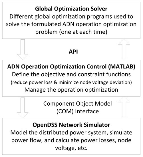
Figure 1.
Framework of co-simulation platform.
The objective and constraint functions of the ADN operation optimization are defined in the Optimization Control Module using MATLAB codes. Two-way data exchange through network control variables or optimization design variables are done between the Optimization Control Module that assesses progress of the optimization search and the OpenDSS Network Simulator that simulate network power flow. The data exchanges are carried out through the Component Object Model (COM) interface provided by the OpenDSS package between the Optimization Control Module and the OpenDSS; and the API between the Optimization Control Module and the generic Global Optimization Solver. The Operation Optimization Control module passes intermediate values of the design variables to OpenDSS, and OpenDSS runs the power flow simulation of the distribution system over successive time intervals and calculates the power loss while satisfying bus voltage and power balance. The power flow simulation results are then fed back to the Control Module for next global optimization search iteration using the Global Optimization Solver until the stopping criteria of the optimization are satisfied.
4.4. Operation Optimization Procedure
A flowchart for illustrating the data flow among the three major parts of the simulation-based network operation optimization platform is shown in Figure 2. The detailed solution procedure steps are described as follows:
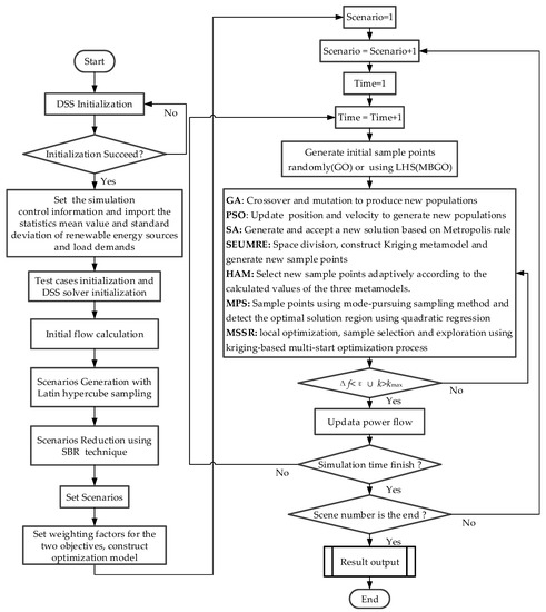
Figure 2.
ADN operation optimization considering uncertainties using various optimization algorithms.
Step 1: Initialize the connection between OpenDSS simulator and MATLAB, if successful, then enter the second step, otherwise, continue to establish communication connection.
Step 2: Set the simulation control variables, and import the statistics mean value and standard deviation of DGs and load demands based on the observed value
Step 3: Initialize the DSS test case file and define the controlled element object, then calculate the initial power flow.
Step 4: Generate the probability scenarios using Latin hypercube sampling (LHS) method, reduce the scenarios and determine the corresponding scenario probability with the SBR (Synchronous Back to Generation Reduction) technique.
Step 5: Define the total scenarios and set weighting factors and for the two objectives to be optimized (nodes voltage deviation, or active power loss, or both), then convert the constrained optimization problem into an unconstrained optimization problem as described by Equations (19)–(23), set scenario = 1, and time = 1.
Step 6: For each scenario, each time interval, generate a number of initial populations randomly for the conventional metaheuristic global optimization (GO) methods, or generate initial sample points using the LHS for the MBGO methods.
Step 7: Search for new solutions: for the GA algorithm, use crossover and mutation to produce new populations. For the PSO algorithm, update position and velocity of current populations based on their personal experience as well as information gained through interactions to generate new populations. For the SA algorithm, generate a new solutions randomly and determine whether to accept it based on Metropolis rule. For the SEUMRE algorithm, divide the design space into several unimodal regions; identify and rank the regions, then fit a Kriging model and identify its minimum. For the HAM algorithm, select several new sample points adaptively according to the calculated values of the three metamodels and update the current best solution. For the MPS algorithm, sample a number of points using mode-pursuing sampling method and detect the optimal solution region using quadratic regression. For the MSSR algorithm, use a kriging-based multi-start optimization process to carry out the local optimization, sample selection and exploration alternately, and then select better sample points to supplement the kriging model and identifies the current optimal solution.
Step 8: Stopping criteria: check whether the relative error () between the last two optimal solutions is less than a given value (ε) or the current number of iterations () is greater than the set value (). If satisfied, update the power flow; otherwise, return to Step 7.
Step 9: Check the simulation time, if the simulation time reaches the end, go to Step 10, otherwise, return to Step 6.
Step 10: Check the scenario number, if the scenario number reaches the end, output the results, otherwise, return to Step 6.
Step 11: Close the connection between OpenDSS simulator and control, produce charts using obtained results, analyze and discuss the results.
5. Case Studies
5.1. IEEE 13 Node System—A Small Distribution Network
5.1.1. Network Structure and Results of the Optimization
The first selected test case is a modified IEEE 13 node system, a small and highly loaded 4.16 kV grid that is revised from its original form [42] for this research, as shown in Figure 3. Its distributed power generations, included MT, diesel generator (DS), FC, PV and WT, are connected at nodes 671, 670, 675, 645 and 634, respectively. The 24 h observed mean and variance of wind speed and illumination intensity are assumed to be taken from reference [30], by which the corresponding wind speed Weibull distribution parameters and illumination intensity beta distribution parameters can be calculated. Load demand power assumed to meet the normal distribution [30], the final probability scenarios of wind power, PV and load demand using the scenario generation and scenario reduction methods are shown in Figure 4a–c, the probability distribution of each scenario is shown in Figure 4d, and the parameters of the distributed power generation system are given in Table 1.
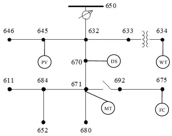
Figure 3.
Modified IEEE 13 node test case.
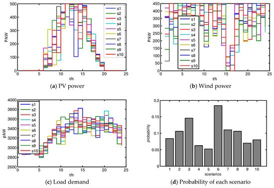
Figure 4.
The probability scenarios of PV, wind power and load demand using the scenario generation and scenario reduction methods (a) PV; (b) wind power; (c) Load demand; and (d) probability of each scenario.

Table 1.
Parameters of distributed power generations.
The model ADN simulation and optimization have been carried out on a regular PC equipped with an Intel(R) Core(TM) i5-5200 2.2-GHz CPU, 8-GB memory, and the Windows 7 operating system. The parameters of the tested GO and the selected MBGO algorithms are set as follows: the initial sampling size of the SEUMRE algorithm , the “cheap” sample size m = 300, the Kriging metamodel correlation function parameters: , , , the convergence criteria , the maximum number of iterations . The initial sampling points of HAM algorithm is set to 8, the number of cheap points for HAM algorithm is set to 10,000, the number of promising points is set to 7, the Kriging metamodel correlation parameters for HAM are the same as SEUMRE, the number of points in the data set and the degree of the full polynomial surface for the polynomial response surface model in HAM is set to 5 and 2, respectively, the parameter c value, the polynomial term and the verbose value for the radial basis function model is set to 1, 0 and 1, respectively, the convergence criteria of HAM is set to , the maximum number of iterations . For the MSSR algorithm, the initial sampling points is 8, the size of the reduced medium space and the local space is 30 and 5 respectively, the Kriging correlation parameters, the convergence criteria and the maximum number of iterations are the same as SEUMRE. For the MPS algorithm, the number of initial samples is set to 11, the number of samples selected from each time sampling is also set to 11, the number of the coefficients for fitting a second-order function is set to 10, the convergence criteria , the maximum number of iterations . The mutation probability of genetic algorithm is Pmg = 0.01, crossover probability Pmc = 0.8, the initial population size 50, the convergence criteria , the max iterations number is set to 200. The initial population of particle swarm optimization algorithm is 20, the maximum inertial weight ws = 0.9, the minimum inertia weight we = 0.4, the learning factor is C1 = C2 = 2, the convergence criteria , the max iterations number is 200. The initial temperature of the simulated annealing algorithm is T0 = 100, and the annealing rate is λ = 0.85, the convergence criteria , the max iterations number is also set to 200. Table 2 presents the results of the tested representative GO and the selected MBGO algorithms in solving the ADN operation optimization problem, NFE is the number of function evaluations of the design objective. The obtained optimization results, the computation time, and needed NFE of each of the six global optimization algorithms are shown in Table 2 and Figure 5.
Table 2.
Performance comparison among tested global optimization algorithms for the IEEE 13 node test case.
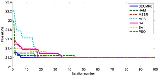
Figure 5.
Convergence comparison of the tested optimization algorithms for IEEE 13 node test case.
5.1.2. Computation Time and NFE Measures on Computation Efficiency of Optimization Techniques
This study showed that all six global optimization methods can converge to the global optimum of this discontinuous objective function with multiple local minima, although their convergence performance varies significantly. Two different measures on computational efficiency are used, computation/running time and number of (objective) function evaluation (NFE) for the following reasons:
- The needed computation time shows the feasibility of the approach for real-time optimal and dynamics network operation control and scheduling for this given problem. The measure is only important for computation intensive problem and for solution time-constrained real-time applications.
- The needed NFE, as an impartial measure shows the relative computation efficiency of the algorithm, regardless of the computation intensity of the objective function and the capability of the used computer. Specifically it indicates the potential of the approach to be used for more complex ADN network optimization problem.
Due to the small size of this tested network and the simplicity of operation scheduling task, the computation time needed to evaluate the objective function is short although its NFE varied considerably, as shown in Table 2. This test case is a black-box global optimization problem, but not a computation intensive problem. On the other hand, the ADN network planning optimization problem is both a black-box global optimization problem and a computation intensive problem. Since the latter needs to consider various network designs under their optimal operations and each design data point requires NFE times of operation scheduling objective function evaluation, the design optimization, as a nested design optimization problem requiring hundreds or thousands of design points in its search of the design optimum, will require hundred or thousand times of NFE of the optimal operation scheduling objective function evaluation. The network design and planning optimization problem will be really computation intensive. The ability of different optimization techniques to handle this hidden issue can only be measured by the NFE in this test case.
5.1.3. Test Case 1 Result Analysis and Discussion
The test results shown in Table 2 and Figure 5 indicated that the SEUMRE method required much less computational time and converged much faster than the traditional GO optimization techniques. The CPU time needed by the SEUMRE method is only 11.03% of GA and 14.52% of PSO in average, showing the effectiveness of the SEUMRE algorithm in dealing with low dimensional ADN operation optimization problem. The SEUMRE method can identify global optimum efficiently using a small number of simulation sample points and optimization search iterations. On the other hand, the HAM, MPS and MSSR method required much longer computation time although their NFE remained low. Considerable computation has been devoted to form the metamodels in their search of the global optimum. Due to the simplicity of the network and modest computation needed in its network simulation, the multiple metamodels used in HAM and the multiple starting schemes used in MSSR added additional computation burden while their advantages in search robustness and flexibility have not yet able to show. Nevertheless, all three MBGO methods showed much lower needed NFEs and great advantage for more computation intensive ADN design optimization problem as discussed in the previous subsection.
5.1.4. Considerations on Multiple and Competing Optimization Objectives
In this study, different weight ratios on the two competing objectives of the operation optimization have also been tested using the MBGO algorithms. Figure 6 shows the network performance result comparison with and without the optimal operation control in one day simulation using different weights on the combined objective function, for pure active power loss minimization (w1 = 0 and w2 = 1), for node voltage deviation minimization (case w1 = 1 and w2 = 0), and for both active power loss and node voltage deviation minimizations (w1 = 100 and w2 = 1). The DG with optimized dispatch operation has significantly reduced power loss of the network system with considerably reduced cost of the ADN operation. This comparison on the three different operation optimization scenarios showed slightly different levels of power loss reduction in the order of active power loss minimization, power loss and node voltage deviation minimization, and node voltage deviation minimization, directly related to the chosen weights on the overall design objective. This formulation with flexible weight selection supports different operation control intents, and appropriate weight coefficients should be carefully selected for an actual ADN optimal operation application.
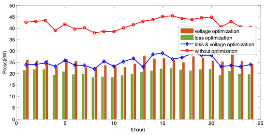
Figure 6.
Average power loss with and without optimal control in one-day simulation for IEEE 13 test case.
Figure 7 presents the voltage variation of node 634 in one day simulation with and without the optimal operation control. The node voltage fluctuation has been effectively alleviated by the global optimization, allowing the network to receive more fluctuating power from distributed renewable energy sources and to have a higher proportion of clean energy.
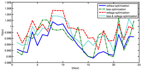
Figure 7.
Voltage variation at the Node 634 in one day simulation for IEEE 13 node test case.
The choice and weight of the design objective also has considerable impact on the voltage fluctuation control in the order of node voltage deviation minimization, power loss and node voltage deviation minimization, and active power loss minimization, as shown in Figure 6. It is thus important to choose appropriate weight coefficients in the multi-objective optimal operation from the network control perspective as well.
Figure 8 shows the voltage distribution of all 13 nodes during a selected time period, and three different cases are discussed, case one without optimal control, case two with optimal control but not consider the uncertainties of DGs and loads, case three with optimal control and consider the uncertainties. We can find that the optimization reduced voltage deviation at different nodes and stabilized voltage in the network. Also, it can be found that after considering the uncertainties of DGs and loads, the system can cope with a variety of possible uncertainty scenarios and the voltage stability is better.
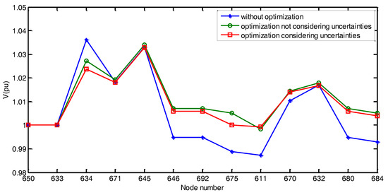
Figure 8.
Node voltage distribution of the IEEE 13 node test case.
5.2. IEEE 33 Node System—A Medium-Size Distribution Network
The ADN test case is a 33-bus, 12.66-kV, radial distribution system [43] as shown in Figure 9, consisting of 33 nodes and 32 lines. The line and load data of the network are obtained from [44], and the total real and reactive power loads on the system are 3.715 MW and 2.300 MVAr, respectively. The initial power loss of this system is 202.771 kW, the range of node voltage is set to be 0.95~1.05 pu, the upper limit of transmission line current is set to be 0.3 kA. The lowest bus bar voltage is 0.9661 pu, occurring at the Node 18. Eight DGs including one PV power generation unit, one wind turbine power generation unit, three micro-turbine (MT) units and three fuel cell (FC) units are attached to the Node 8, 12, 18, 6, 28, 33, 25 and 22, respectively. Besides that, two battery energy storage system (ESS), rated power of 1.0 MW and 0.5 MW, are attached to the Node 23, and 20 of the network system, respectively. The detail technical parameters of each DG and ESS are given in Table 3 and Table 4. The probability scenarios of WT, PV, and the load demand are assumed to be the same with test case 1.
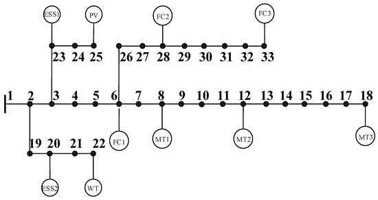
Figure 9.
Modified IEEE 33 node test case.
Table 3.
Key parameters of distributed power generation.
Table 4.
Key parameters of distributed energy storage system.
The parameters of the GO and the MBGO algorithms are basically set the same as test case 1, except the initial sampling size of the SEUMRE and MPS algorithms, where they are set to be 45 and 46, respectively for this medium-scale test case. Table 5 presents the results obtained from the 33 node ADN system operation optimization problem, using different GO optimization programs. The numbers of function evaluation of these methods are shown in Figure 10.
Table 5.
Performance comparison among the different global optimization methods for IEEE 33 node test case.
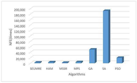
Figure 10.
NFE comparison of global optimization methods for the IEEE 33 node test case.
From the results in Table 5 and Figure 10, we can find that for more complex networks and optimization models, SEUMRE algorithm is still the algorithm with the highest computational efficiency, it introduce the metamodel and use of the cheap points of the metamodel to replace the computationally expensive sample point evaluation on the original model, the number of function evaluations of it is then greatly reduced compared to that of the traditional stochastic search algorithms, and thus the computation time is decreased and the computational efficiency is improved. In this test case study, it can be found that although the NFEs of the HAM, MPS and MSSR algorithms are much less than the traditional global optimization algorithms, but the additional computation burdens caused by the multiple metamodels used in HAM and the multiple starting schemes used in MSSR are still higher than the decrease of objective function evaluation time, so the net computation time showed no advantage in this ADN operation scheduling optimization problem. Only when the objective function evaluation is more “expensive” as in the ADN design optimization problem discussed previously in Section 5.1.2, the advantages of the MBGO algorithms, indicated by their considerable lower NFE, will be more prominent.
We can use an example of ADN design optimization considering optimal ESS size to show the importance of the NFE measure and the advantage of the MBGO techniques. In the above operation optimization model a given size ESS has been considered. To find a better network design with the optimally sized ESS, a top layer network design optimization can be added to the current network operation model, using the ESS size as the only design variable. A two-level, nested optimization model is thus formulated, and the needed computation of the new design optimization objective function at the top level is much more intensive. The optimization problem is now of both black-box and computation intensive types. Using the six MBGO and traditional GO algorithms to solve this new ADN ESS size design optimization problem led to the results shown in Table 6.
Table 6.
Results of network ESS size design optimization for the IEEE 33 node ADN test case under optimal operation.
For this complex and computation intensive ADN ESS design optimization problem, all three MBGO algorithms showed superior computational efficiency with much less NFE and shorter computation time. This simple test illustrated the inherent limitation of the conventional GO algorithms and the advantage of the MBGO techniques. For the ADN design optimization with much more design variables for varying network architecture and component sizes, the advantages of MBGO techniques will be much more significant. These challenging design optimization problems are studied by the authors at present and are beyond the scope of this paper.
The power losses in one day operation simulation with different operation scenarios are shown in Figure 11. The optimized operation of this medium scale ADN presented significant system loss reduction of 62.5% and improved system efficiency, regardless of the selection of the optimal operation scenarios.
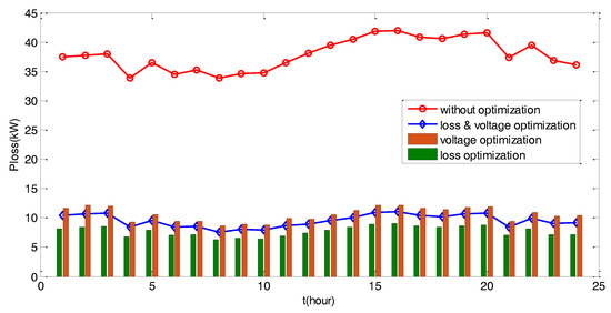
Figure 11.
Power loss in one day simulation for the IEEE 33 node test case.
The simulation results on voltage variation at Node 22 in one day operation with different optimal operation scenarios, determined by different weight coefficients of the objective function, are given in Figure 12. Without the optimization, node voltage changes dramatically with time, between 0.997~1.003 pu. Under optimal operation with optimized active and reactive power output of DGs and ESSs, the node voltage fluctuation dropped considerably with a stable voltage value in the vicinity of 1 pu. The test has proved the advantage of the proposed network operation optimization model and solution methods in effectively improving network voltage quality.
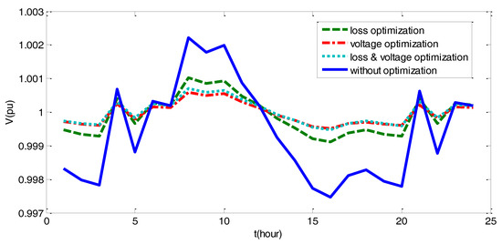
Figure 12.
Node 22 voltage variation in one day simulation for the IEEE 33 node test case.
Voltage distribution among the 33 nodes of the network at a representative time section is shown in Figure 13. Without the optimal control, the voltage at the end of the feeder (Node 18 and Node 33) has fallen to near 0.96 pu. The operation optimization coordinately injected power from the three MTs and three FCs to improve the quality of power supply at the feeder terminal nodes, leading to ideal feeder voltage around 1 pu. The two ESS devices are mainly responsible for the high permeability caused by PV and WT to absorb excess inductive reactive power, intermittent fluctuations and stabilize PV and WT power charge, and ensuring safe and reliable operation of the network system.
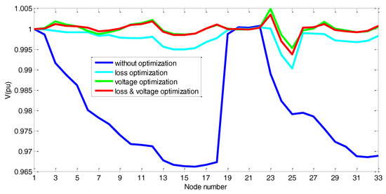
Figure 13.
Node voltage distribution with and without operation optimization for the IEEE 33 node test case.
5.3. IEEE 123 Node System—A Large-Scale Distribution Network
To test the applicability of different global optimization methods to large-scale distribution systems, the IEEE 123-bus radial distribution feeder case [45], as shown in Figure 14, was used as the third test case. In this ADN system, the three-phase power base is 5MVA while the line-to-line voltage base is 4.16 kV, the network consists of 123 nodes and 117 lines. The line and load data of the network were obtained from [46], the maximum and minimum voltage limits at each node are 1.05 and 0.95 pu, respectively. One PV power generation unit with the rated capacity of 100 kW and one wind turbine power generation unit with the rated capacity of 120 kW are attached to Node 83 and Node 22 respectively, eight micro gas turbine (MT) systems, six hydrogen fuel cell systems (FC), and six diesel generators (DS), are also embedded into the network system to handle power fluctuations from the PV and WT systems. The major technical parameters and access modes of each DG are shown in Table 7. The probability scenarios of WT, PV, and the load demand are the same with test case 1.
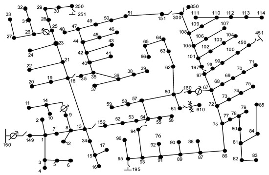
Figure 14.
IEEE 123 node test case.
Table 7.
Parameters of distributed power generation in IEEE 123 test case.
The parameters of all the algorithms are set the same as test case 1, the initial sampling size of the SEUMRE and MPS algorithm are 210 and 211, respectively. The test results from the operation optimization of the 123 node, large-scale ADN system, using the six different global optimization methods are given in Table 8.
Table 8.
Performance comparison of seven global optimization methods for the IEEE 123 node test case.
The operation optimization of the IEEE 123 node large-scale distribution system presented a different type of global optimization problem due to its large number of design variables and large search space, regardless of the same form of objective and constraint functions of the optimization formulation. The test results, shown in Table 6, present the different performance behaviors of the tested global optimization methods, comparing with the previous small- and medium-sized ADN operation optimization. The results showed that all three MBGO algorithms needed longer computation time, while the conventional GO algorithms converged to satisfactory results quicker. High dimensionality caused intractability of systematic searching through vast design space and approximation of the original, high-dimensional objective functions required exponentially increased number of sample points. The three surrogate model based MBGO methods narrowed down the search to specific regions too quickly, leading to repeated efforts in identifying the “most promising” region. While the three stochastic GO methods randomly sampled the entire search space, progressed slowly, but surely, producing the final search results in relatively shorter time. In addition, all six GO search methods require considerable solution time in identifying the optimal operation solution of the large ADN, and it becomes difficult or impossible to use this optimization method directly for real-time optimal ADN operation control and dynamic scheduling. Possible solutions to this problem include the less desirable path of using much more powerful computers; and the possible alternative of using a simple real-time, network load scenario pattern matching method to retrieve previously generated solution from the optimal ADN operation solution database that has been created off-line through intensive ADN operation optimizations for various possible load scenarios. The latter approach is part of our present research and again beyond the scope of this paper.
The findings from this research allows us to intelligently select different global optimization tools for different size of network operation optimization problems, and to introduce more advanced MBGO algorithms to address the issue. There is no simple one-size-fit-all solution for the optimal scheduling and design of various types and sizes of power distribution networks. For different scale ADN operation optimization problems, it is important to select the appropriate global solution tools accordingly. MBGO algorithms are more suitable for small- and medium-scale distribution system operation optimization; and for large-scale ADN operation optimization problem, the traditional GO algorithms are the preferable choices at present.
The power loss of different network operation scenarios for the IEEE 123 node test case is shown in Figure 15. The optimized operation of the large-scale ADN, solved using the conventional GO methods, presented much reduced system power loss of almost 68.3%.
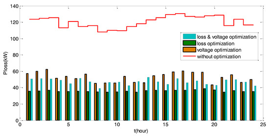
Figure 15.
Power loss for the large-scale ADN in one day simulation for the IEEE 123 node test case.
Voltage distribution of the IEEE 123 node test case with and without optimal control is shown in Figure 16. The optimal control considerably reduced voltage deviation at all nodes through network wide optimization. The voltage deviation minimization and power loss minimization operation scenarios led to single-minded results, while the combined voltage deviation and power loss minimization operation scenario led to balanced operation and better overall control effect.
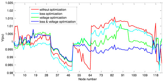
Figure 16.
Node voltage distribution for the IEEE 123 node test case.
6. Conclusions
Optimal operation scheduling of active distribution networks (ADNs) is one of the key technologies to improve the operation efficiency of the active distribution network and to promote the efficient utilization of renewable energy. In this work, an ADN operation scheduling optimization problem with fully consideration of the uncertainties of distributed generations and loads has been introduced to reduce system power loss and minimize voltage deviation. The formulated optimization problem has been applied to three representative ADNs of different sizes: small-, medium- and large-scale, with 13, 33 and 123 nodes, modified from the standard IEEE test cases. Representative global optimization methods, both of the conventional, stochastic type and the more recently introduced MBGO kind have been used as solution methods for solving the operation optimization problems in a comparative study to better understand their advantages, drawbacks and limitations, and to provide guidelines for subsequent scheduling, planning and design optimization of ADNs. These include the three well-known stochastic and evolutionary GO methods, SA, GA and PSO, and the four MBGO methods, SEUMRE, HAM, MPS and MSSR. The computational efficiency, measured by computation time and NFE, and the global convergence of these methods are analyzed and discussed in details. The results from the network operation optimization and their comparisons showed that global optimization techniques can replace the less capable or even inadequate conventional optimization methods to effectively identify the optimal ADN operation solutions and to form the foundation for the optimal planning and design of ADN.
The comparisons produced guidelines on the applicability and suitability of each of these optimization methods to different classes of ADN operation optimization problems. For small-scale and medium-scale ADN operation optimization problems, search for the optimal operation solutions can be successfully and quickly carried out using the recently introduced MBGO methods. These algorithms can considerably reduce the computation time needed for solving these complex, black-box, global optimization problems, making operation scheduling optimization feasible for practical use. When the number of design variables is small, real-time operation scheduling might be feasible due to the short solution time needed. On the other hand, for large-scale ADN operation optimization problems with a large number of design variables, the MBGO methods required much more computation time to converge to the global optimum and showed inferior computation efficiency than the conventional stochastic global optimization methods. The high dimension problems with a large number of network nodes lead to exponential increase of sampling space size and possible numbers of local minima. The amount of computation for forming the meta-models in the three tested MBGO methods also increase sharply, leading to low search efficiency. The stochastic global optimization methods, due to their steady search schemes, present stable convergence and steady performance in dealing with these large scale problems. The MBGO algorithm is more suitable for small- and medium-scale ADN operation and planning design problem, and the evolutionary GO algorithm more effectively in large-scale ADN operation and planning and design issues. This research has shown ways to formulate and solve the challenging network operation scheduling global optimization problem. The optimal control of DGs and ESSs in active distribution network can effectively reduce network power loss and voltage deviation to ensure the economical operation of distribution network and guarantee the voltage stability of the system.
The NFE measures, reordered in the tests, also demonstrated the great benefits and potential of the MBGO methods in more challenging optimal operating ADN’s design optimization problems and other computation intensive tasks, through the optimal ESS sizing example. The method of optimal operating ADN’s design optimization is briefly discussed.
In this work, the challenging global optimization task of large ADN operation scheduling problem based on the IEEE 123 node test case has also been successfully completed, presenting a new path for finding the optimal solution of large adaptive grid scheduling. Meanwhile, a possible path for dealing with the high-dimensional ADN’s optimal scheduling problems have been briefly mentioned as possible future research.
Acknowledgments
This work was supported by the National Natural Science Foundation of China (51607170), the Canada-China Clean Energy Partnership Initiative, the Key Front Science Project of Chinese Academy of Sciences (QYZDB-SSW-JSC024), the National High Technology Research and Development Program (“863” Program) of China (2015AA050402) and the International Collaboration Programs of the Chinese Academy of Sciences and the Foreign Expert Affairs.
Author Contributions
Hao Xiao, Wei Pei and Zuomin Dong conceived and designed the study; Hao Xiao performed the study and wrote the paper; Zuomin Dong, Li Kong and Dan Wang reviewed and edited the manuscript. All authors read and approved the manuscript.
Conflicts of Interest
The authors declare no conflict of interest.
References
- McDonald, J. Adaptive intelligent power systems: Active distribution networks. Energy Policy 2008, 36, 4346–4351. [Google Scholar] [CrossRef]
- Zhigljavsky, A.; Zilinskas, A. Stochastic Global Optimization; Springer Science & Business Media: Berlin, Germany, 2007; Volume 9. [Google Scholar]
- Ezzati, S.M.; Vahedi, H.; Yousefi, G.R.; Pedram, M.M. Security Constrained Optimal Power Flow Solved by Mixed Integer Non Linear Programming. Int. Rev. Electr. Eng. 2011, 6, 3051–3057. [Google Scholar]
- Wibowo, R.S.; Maulana, R.; Taradini, A.; Pamuji, F.A.; Soeprijanto, A.; Penangsang, O. Quadratic Programming Approach for Security Constrained Optimal Power Flow. In Proceedings of the 2015 7th International Conference on Information Technology and Electrical Engineering (ICITEE), Chiang Mai, Thailand, 29–30 October 2015; pp. 200–203. [Google Scholar]
- Ferreira, R.S.; Borges, C.L.T.; Pereira, M.V.F. A Flexible Mixed-Integer Linear Programming Approach to the AC Optimal Power Flow in Distribution Systems. IEEE Trans. Power Syst. 2014, 29, 2447–2459. [Google Scholar] [CrossRef]
- El Ela, A.A.A.; Abido, M.A.; Spea, S.R. Optimal power flow using differential evolution algorithm. Electr. Power Syst. Res. 2010, 80, 878–885. [Google Scholar] [CrossRef]
- Hazra, J.; Sinha, A.K. A multi-objective optimal power flow using particle swarm optimization. Eur. Trans. Electr. Power 2011, 21, 1028–1045. [Google Scholar] [CrossRef]
- Todorovski, M.; Rajicic, D. An initialization procedure in solving optimal power flow by genetic algorithm. IEEE Trans. Power Syst. 2006, 21, 480–487. [Google Scholar] [CrossRef]
- Kahourzade, S.; Mahmoudi, A.; Mokhlis, H.B. A comparative study of multi-objective optimal power flow based on particle swarm, evolutionary programming, and genetic algorithm. Electr. Eng. 2015, 97, 1–12. [Google Scholar] [CrossRef]
- Lo, C.H.; Chung, C.Y.; Nguyen, D.H.M.; Wong, K.P. A parallel evolutionary programming based optimal power flow algorithm and its implementation. In Proceedings of the 2004 International Conference on Machine Learning and Cybernetics, Shanghai, China, 26–29 August 2004; Volume 1–7, pp. 2543–2548. [Google Scholar]
- Niknam, T.; Narimani, M.R.; Jabbari, M. Dynamic optimal power flow using hybrid particle swarm optimization and simulated annealing. Int. Trans. Electr. Energy Syst. 2013, 23, 975–1001. [Google Scholar] [CrossRef]
- Duman, S.; Guvenc, U.; Sonmez, Y.; Yorukeren, N. Optimal power flow using gravitational search algorithm. Energy Convers. Manag. 2012, 59, 86–95. [Google Scholar] [CrossRef]
- Radosavljevic, J.; Jevtic, M.; Arsic, N.; Klimenta, D. Optimal power flow for distribution networks using gravitational search algorithm. Electr. Eng. 2014, 96, 335–345. [Google Scholar] [CrossRef]
- Abido, M.A. Optimal power flow using tabu search algorithm. Electr. Power Compon. Syst. 2002, 30, 469–483. [Google Scholar] [CrossRef]
- Ayan, K.; Kilic, U. Solution of Multi-Objective Optimal Power Flow with Chaotic Artificial Bee Colony Algorithm. Int. Rev. Electr. Eng. 2011, 6, 1365–1371. [Google Scholar]
- Ghasemi, M.; Ghavidel, S.; Ghanbarian, M.M.; Massrur, H.R.; Gharibzadeh, M. Application of imperialist competitive algorithm with its modified techniques for multi-objective optimal power flow problem: A comparative study. Inf. Sci. 2014, 281, 225–247. [Google Scholar] [CrossRef]
- Weise, T.; Wu, Y.Z.; Chiong, R.; Tang, K.; Lassig, J. Global versus local search: The impact of population sizes on evolutionary algorithm performance. J. Glob. Optim. 2016, 66, 511–534. [Google Scholar] [CrossRef]
- Montenegro, D.; Hernandez, M.; Ramos, G.A. Real Time OpenDSS framework for Distribution Systems Simulation and Analysis. In Proceedings of the 2012 Sixth IEEE/PES Transmission and Distribution: Latin America Conference and Exposition (T&D-La), Montevideo, Uruguay, 3–5 September 2012. [Google Scholar]
- Kvasov, D.E.; Sergeyev, Y.D. Deterministic approaches for solving practical black-box global optimization problems. Adv. Eng. Softw. 2015, 80, 58–66. [Google Scholar] [CrossRef]
- Kvasov, D.; Menniti, D.; Pinnarelli, A.; Sergeyev, Y.D.; Sorrentino, N. Tuning fuzzy power-system stabilizers in multi-machine systems by global optimization algorithms based on efficient domain partitions. Electr. Power Syst. Res. 2008, 78, 1217–1229. [Google Scholar] [CrossRef]
- Younis, A.; Dong, Z.M. Trends, features, and tests of common and recently introduced global optimization methods. Eng. Optim. 2010, 42, 691–718. [Google Scholar] [CrossRef]
- Li, L.; Dong, J.; Dong, J.G.; Yu, B.; Peng, J.C.; He, J.B. Prediction of the spatial distribution of bovine endemic fluorosis using ordinary kriging. Bull. Vet. Inst. Pulawy 2015, 59, 161–164. [Google Scholar] [CrossRef]
- Fang, H.B.; Horstemeyer, M.F. Global response approximation with radial basis functions. Eng. Optim. 2006, 38, 407–424. [Google Scholar] [CrossRef]
- Wang, G.G.; Shan, S. Review of metamodeling techniques in support of engineering design optimization. J. Mech. Des. 2007, 129, 370–380. [Google Scholar] [CrossRef]
- Dong, H.; Song, B.; Dong, Z.; Wang, P. Multi-start Space Reduction (MSSR) surrogate-based global optimization method. Struct. Multidiscip. Optim. 2016, 54, 906–926. [Google Scholar] [CrossRef]
- Shan, S.; Wang, G.G. Survey of Modeling and Optimization Strategies for High-Dimensional Design Problems. In Proceedings of the AIAA/ISSMO Multidisciplinary Analysis and Optimization Conference, Victoria, BC, Canada, 10–12 September 2008; pp. 184–194. [Google Scholar]
- Haftka, R.T.; Villanueva, D.; Chaudhuri, A. Parallel surrogate-assisted global optimization with expensive functions—A survey. Struct. Multidiscip. Optim. 2016, 54, 3–13. [Google Scholar] [CrossRef]
- Chellali, F.; Khellaf, A.; Belouchrani, A.; Khanniche, R. A comparison between wind speed distributions derived from the maximum entropy principle and Weibull distribution. Case of study; six regions of Algeria. Renew. Sustain. Energy Rev. 2012, 16, 379–385. [Google Scholar] [CrossRef]
- Ettoumi, F.Y.; Mefti, A.; Adane, A.; Bouroubi, M.Y. Statistical analysis of solar measurements in Algeria using beta distributions. Renew. Energy 2002, 26, 47–67. [Google Scholar] [CrossRef]
- Sobu, A.; Wu, G. Optimal operation planning method for isolated micro grid considering uncertainties of renewable power generations and load demand. In Proceedings of the 2012 IEEE Innovative Smart Grid Technologies-Asia (ISGT Asia), Tianjin, China, 21–24 May 2012; pp. 1–6. [Google Scholar] [CrossRef]
- Singh, R.; Pal, B.C.; Jabr, R.A. Statistical representation of distribution system loads using Gaussian mixture model. IEEE Trans. Power Syst. 2010, 25, 29–37. [Google Scholar] [CrossRef]
- Iman, R.L. Latin Hypercube Sampling; Wiley Online Library: Hoboken, NJ, USA, 2008. [Google Scholar]
- Owen, A.B. Controlling correlations in Latin hypercube samples. J. Am. Stat. Assoc. 1994, 89, 1517–1522. [Google Scholar] [CrossRef]
- Growe-Kuska, N.; Heitsch, H.; Romisch, W. Scenario reduction and scenario tree construction for power management problems. In Proceedings of the 2003 IEEE Bologna Power Tech Conference, Bologna, Italy, 23–26 June 2003; Volume 3, p. 7. [Google Scholar]
- Mohammadi, S.; Soleymani, S.; Mozafari, B. Scenario-based stochastic operation management of microgrid including wind, photovoltaic, micro-turbine, fuel cell and energy storage devices. Int. J. Electr. Power Energy Syst. 2014, 54, 525–535. [Google Scholar] [CrossRef]
- Kirkpatrick, S.; Gelatt, C.D.; Vecchi, M.P. Optimization by Simulated Annealing. Science 1983, 220, 671–680. [Google Scholar] [CrossRef] [PubMed]
- Holland, J.H. Genetic Algorithms. Sci. Am. 1992, 267, 66–72. [Google Scholar] [CrossRef]
- Kennedy, J.; Eberhart, R. Particle swarm optimization. In Proceedings of the 1995 IEEE International Conference on Neural Networks, Perth, Australia, 27 November–1 December 1995; Volume 1–6, pp. 1942–1948. [Google Scholar]
- Younis, A.; Dong, Z.M. Metamodelling and search using space exploration and unimodal region elimination for design optimization. Eng. Optim. 2010, 42, 517–533. [Google Scholar] [CrossRef]
- Gu, J.; Li, G.Y.; Dong, Z. Hybrid and adaptive meta-model-based global optimization. Eng. Optim. 2012, 44, 87–104. [Google Scholar] [CrossRef]
- Wang, L.Q.; Shan, S.Q.; Wang, G.G. Mode-pursuing sampling method for global optimization on expensive black-box functions. Eng. Optim. 2004, 36, 419–438. [Google Scholar] [CrossRef]
- Paudyal, S.; Canizares, C.A.; Bhattacharya, K. Optimal Operation of Distribution Feeders in Smart Grids. IEEE Trans. Ind. Electron. 2011, 58, 4495–4503. [Google Scholar] [CrossRef]
- Rekha, E.; Sattianadan, D.; Sudhakaran, M. Maximum Loss Reduction and Voltage Profile Improvement with Placement of Hybrid Solar-Wind System. Energy Effic. Technol. Sustain. 2013, 768, 371–377. [Google Scholar] [CrossRef]
- Rao, R.S.; Narasimham, S.V.L.; Raju, M.R.; Rao, A.S. Optimal Network Reconfiguration of Large-Scale Distribution System Using Harmony Search Algorithm. IEEE Trans. Power Syst. 2011, 26, 1080–1088. [Google Scholar]
- Daratha, N.; Das, B.; Sharma, J. Coordination Between OLTC and SVC for Voltage Regulation in Unbalanced Distribution System Distributed Generation. IEEE Trans. Power Syst. 2014, 29, 289–299. [Google Scholar] [CrossRef]
- Kersting, W. Radial distribution test feeders. In Proceedings of the 2001 IEEE Power Engineering Society Winter Meeting, Columbus, OH, USA, 28 January–1 February 2001; Volume 1–3, pp. 908–912. [Google Scholar]
© 2018 by the authors. Licensee MDPI, Basel, Switzerland. This article is an open access article distributed under the terms and conditions of the Creative Commons Attribution (CC BY) license (http://creativecommons.org/licenses/by/4.0/).