Simultaneous Provision of Flexible Ramping Product and Demand Relief by Interruptible Loads Considering Economic Incentives

Abstract

To cope with the net load variability in real time, sufficient ramp capability from controllable resources is required. To address the issue of insufficient ramp capacity in real time operations, flexible ramping products (FRPs) have been adopted by some Independent System Operators (ISOs) in the USA as a new market design. The inherent variability and uncertainty caused by renewable energy sources (RESs) call for new FRP providers apart from conventional generating units. The so-called interruptible load (IL) has proved to be useful in maintaining the supply-demand balance by providing demand relief and can be a viable FRP provider in practice. Given this background, this work presents a stochastic real-time unit commitment model considering ramp requirement and simultaneous provision of IL for FRP and demand relief. Load serving entities (LSEs) are included in the proposed model and act as mediators between the ISO and multiple ILs. In particular, incentive compatible contracts are designed to encourage customers to reveal their true outage costs. Case studies indicate both the system and LSEs can benefit by employing the proposed method and ILs can gain the highest profits by signing up a favorable contract.

1. Introduction

As a new market design to enhance power system operational flexibility, flexible ramping product (FRP) is attracting much attention from both the academic and industry communities. Successful implementations by two ISOs in the United States, i.e., the California ISO (CAISO) and Midcontinent ISO (MISO), have proven the feasibility and practicality of this product [1,2]. FRP is the ramp capability targeting the net system load change between adjacent intervals in real-time (RT) dispatch (e.g., 5-min in CAISO [1] or 10-min in MISO [2]). The net system load, defined as the difference between the actual system load and the total output of variable generation plus scheduled interchanges, always possesses more significant variability and uncertainty than the actual load alone [3]. This issue is exacerbated with the deepening penetration of variable renewable energy sources (RESs). As the “duck curve” [4] shows, several upward/downward steep ramp periods occur in the net load profile of the typical operating day, which calls for more flexible ramping resources to avoid load loss as well as over generation. The “duck curve” is an industry moniker since the shape of the net load profile is very similar to the neck of a duck.

In the present paradigm, only conventional generation units are utilized to provide FRP [2]. However, any RT dispatchable resource can provide such flexible ramping, and thus new potential providers should be explored in order to accommodate the issue of ramp capability shortage caused by the variability and uncertainty of increasing RESs. Several studies have been conducted in recent years to discuss the feasibility of new FRP suppliers, such as obtained from wind and electric vehicles [5,6,7]. By far, few works have explored interruptible load (IL) as a supplier of FRPs. IL is a contract-based demand response program in which the IL customers reduce their load in order to respond to the interruption instructions requested by the ISO when needed (usually during peak periods) [8]. IL can enhance system reliability by providing ancillary services [9] and demand relief [10], improving generation adequacy [11], and alleviating congestion [12]. Owing to its high controllability and fast response, various types of IL programs are used in power system applications. Nevertheless, to the authors’ best knowledge, simultaneous provision of FRP and demand relief by IL has not been studied.

In a competitive electricity market, a load serving entity (LSE) is a profit-seeking organization with granted authority pursuant to local law or regulation to serve its own electrical demands and energy requirements. The LSE aims to maximize its own profit as well as to provide sufficient economic incentives to its managed IL customers. As the mediator between the ISO and multiple IL customers (especially small residential customers), the LSE receives interruption instructions from the ISO and then allocates the total demand relief within its customers in a cost effective way, namely, minimizing the overall outage cost of all customers. The customers’ true outage costs, however, are unknown to the LSE since it is deemed confidential. In [13], the outage cost is constructed as a quadratic function of the amount of curtailed power and the customer type. The customer type, which is private information, is assumed to be discrete and can be estimated based on historical data. Based on that, the cost functions of different customers are calibrated and then used in designing efficient IL contracts. Incentive compatible contracts are designed in [10] to encourage customers to reveal their true cost value of power interruptions and thus enable them to participate in ideal contracts. The outage cost function is quadratic as well, while the customer type is a continuous variable with a given probability distribution. However, these studies in [10] and [13] ignore the limitation of the maximum demand relief a customer can provide and the effect of FRP on it.

IL is deemed as a kind of incentive-based demand response (DR), while the other kind of DR is price-based [14]. A stochastic model is presented in [15] by combining DR and probabilistic wind power forecasting in order to enhance the capability of accommodating wind power in electricity market operation. The DR here is termed as “demand dispatch” and refers in particular to loads with sufficient flexibility to be responsive to prices. The reduction in the load demand during hours with high market prices is similar to the demand relief provided by IL customers. However, the model in [15] does not consider the provision of FRP. The integration of FRP will introduce changes to both the objective function and constraints. For example, the ISO must consider the cost for acquiring sufficient FRPs to meet the system-level ramping capability requirement. On the other hand, market participants may intend to leave a capacity margin for FRP apart from energy and ancillary services. Thus, the mathematical model becomes more complicated when FRP is taken into account. A framework for integrated dispatch of generation and load is presented in [16], with loads modeled as generators by considering the load adjustment cost. The prevailing unit commitment (UC) model is extended to include demand-side participations. However, the work in [16] focuses on large industrial customers and thus neglects the interaction between a LSE and its customers.

This work presents a real-time unit commitment (RTUC) model with IL provision of both FRP and demand relief. The model is run by the ISO in the RT and considers the system-level ramp capability requirement. To cope with the variability and uncertainty of load and RES, the RTUC is modeled stochastically. The optimized dispatching schedule of FRP and demand relief is obtained from the model and regarded as inputs to the IL relief model run by the LSEs. The outage cost function is assumed to be quadratic following [10] and [13], and incentive compensations are adopted as extra motivations to encourage customers to participate in IL programs and consequently choose the proper contract.

The main contributions of this paper are threefold:

(1)

The idea of simultaneous provision of FRP and demand relief by IL is proposed.

(2)

Stochastic RTUC model is presented, taking both ramp capacity requirement and IL provision into consideration.

(3)

Incentive compatible contracts are designed between an LSE and its customers. Additional compensations can help the LSE collect information about customers and thus design special contracts for them.

The remainder of this paper is organized as follows. The concept of FRP and demand relief is presented in Section 2, which also formulates a stochastic RTUC model considering IL provision of these two products. Section 3 describes the IL relief model and the incentive compensation. Section 4 shows the overall process of this work. Case study is demonstrated in Section 5, followed by the conclusions in Section 6.

2. LSE Contributing to System Balance and Flexibility

2.1. Demand Relief

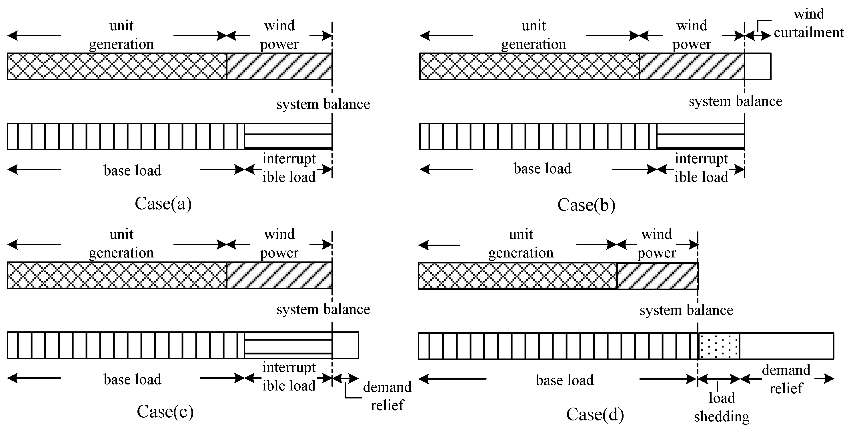
Maintaining generation-demand balance is of great importance for the stable and reliable operation of a power system. This can be achieved by controllable resources on both the supply and demand sides [17]. Figure 1 presents intuitively how a power system with RES keeps balance with the aids of interruptible load in different cases.

Case (a) represents the general situation where the ISO can maintain the balance by adjusting unit generation without reducing RES output or cutting load. When an imbalance materializes as an excess of supply to meet the demand, RES output reduction (e.g., wind curtailment) or conventional generation output reduction may be performed to reduce the supply, as Case (b) shows. On the other hand, if the imbalance materializes as a lack of supply to meet the demand, deployment of reserved conventional units or demand relief from LSEs is required, as Case (c) shows. However, when the deployment of reserved capacity plus the demand relief from all LSEs is still insufficient to cover the supply shortage, base load shedding is performed, as expressed by Case (d). Unlike elastic IL, the value of lost base load is relatively large since the base load is regarded as inelastic and crucial. To avoid such cost, more ILs should be explored as an effective and economical way to maintain system balance.

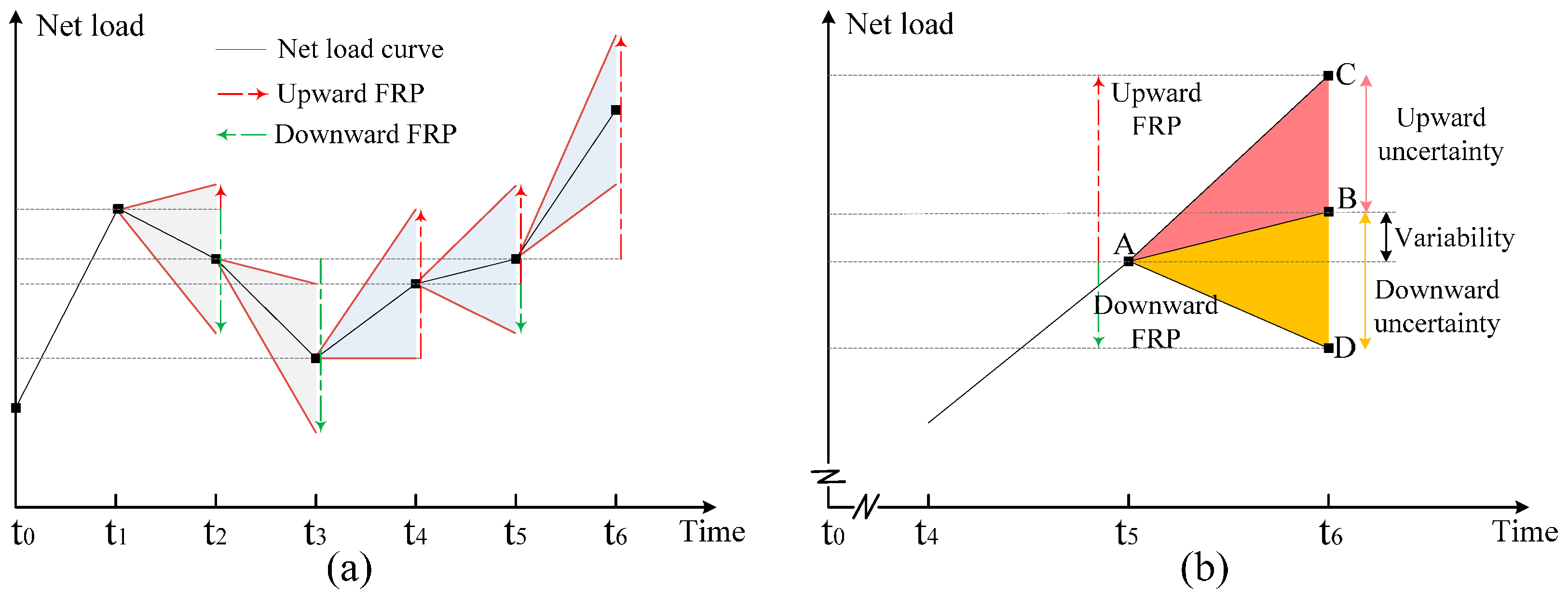
2.2. Flexible Ramping Product

FRP targets the net load movement in RT operations and can be separated into two independent products based on the direction, namely upward FRP and downward FRP. The total FRP provided by all controllable resources should meet the system ramp need. The system-level ramp capability requirements are set for both upward and downward directions for each interval in RT dispatch and can vary between different intervals, as shown in Figure 2a. Note that in t₅, there is only requirement for upward FRP because the net load is expected to increase steeply in this period and no downward FRP is needed. In contrast, only requirement for downward FRP is needed in t₂ and for other intervals such as t₁ and t₄, FRPs for both directions are required. Take t₄ for example, more details are presented in Figure 2b, indicating that ramp capability requirements are composed of the net load variability and surrounding uncertainty. The variability and uncertainty caused by RES raise the requirements and intensify the issue of insufficient ramp capability. Therefore, more controllable resources such as IL are required to be introduced as FRP providers.

The deployment of FRP is embedded into the RT dispatch model. Cleared FRP is reserved at the current interval in order to meet the ramp capability requirement. When energy is dispatched for the next interval, FRP is naturally deployed as energy. Unlike traditional ancillary services whose prices are based on offers, FRP is priced at the opportunity cost for not providing energy and capped by the demand curves [2] prescribed by the ISO. For example, MISO currently adopts a single-step demand curve with the ceiling price being 5 $/MWh [18].

In order to present the technical characteristics of FRP, comparisons between FRP and other traditional ancillary services (e.g., regulation and operating reserve) are made in

Table 1. Comparisons between FRP and regulation as well as operating reserve.

Aspects	Regulation	Operating Reserve	FRP
Function	Manage the instantaneous difference between the actual net load and the forecasted one to ensure the frequency stability	Active power reserved in response to a sudden loss of generation or an unexpected increase of load demand	Ramping capability reserved for addressing the net load changes in future dispatch intervals
Dispatch process	Deployed by Automatic Generation Control (AGC) in a time framework of seconds	Activated only when a contingency event materializes and usually the required response time is within 10–30 min	Deployed every 5 min by a real-time dispatch model
Price	High	relatively high	low
Eligible providers	Able to respond to AGC signals	Able to raise the power output to the targeted level in a required time period	Any real-time dispatchable resource

. FRP is distinguished from regulation and operating reserve in product function, dispatch process, price level and technical requirement. Among these services, regulation has the most rigorous requirement for technologies such as respond speed. For instance, only a quarter of resources in MISO are eligible to provide regulation [19]. On the other hand, providers of operating reserve should be capable of raising their output to the targeted level in required time. In contrast, the technical requirement for providing FRP is the lowest, and any real-time dispatchable resource can provide FRP according to CAISO’s market rule [1]. Although the conventional generators are the only eligible providers of FRP currently in practice, other resources such as demand response can also provide such ramping capability in the RT. Actually, exploring demand-side flexibility could be a better choice if an efficient and reliable demand-side management (DSM) is reached. This is the case because unlike generators which are constrained by ramp rate limits, IL customers can turn off high-power electrical appliances such as heat pump and air conditioner in a very short time. Furthermore, the cost of demand-side resources providing such ramping capability is more effective than conventional generators as demand side is playing increasingly important role in today’s electricity markets. MISO is planning to utilize demand response resources (DDRs) to providing up-ramping capacity by reducing their loads [20].

2.3. Stochastic RTUC Considering System Ramping Requirement and IL Provision

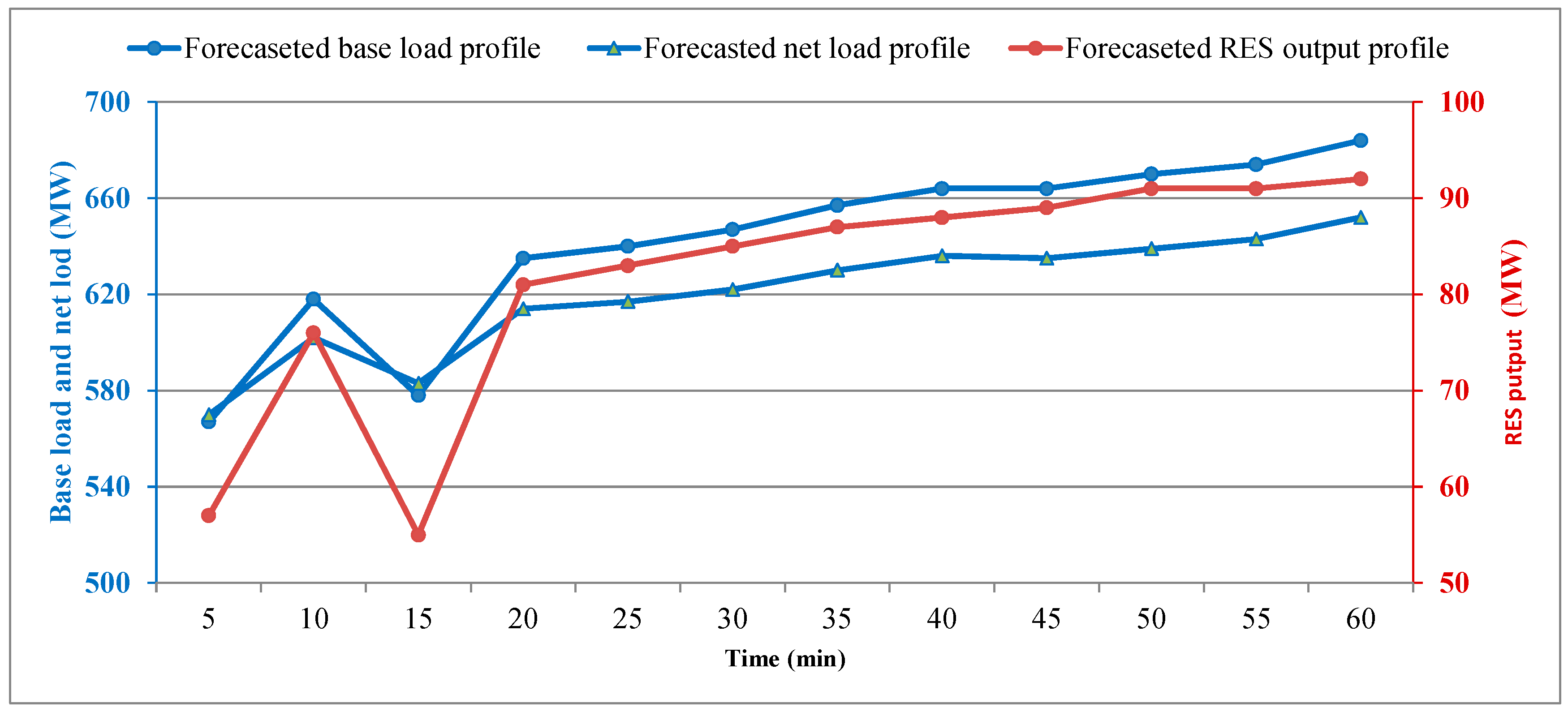
In the RT operation, the ISO endeavors to not only maintain the instantaneous balance, but also to arrange adequate resources to follow the possible net load changes in the near future. Its controllable resources include conventional units and ILs. To cope with the uncertainty of loads and RES outputs, stochastic RTUC is modeled with consideration of system ramping requirement and IL provision. Scenario simulation is performed based on the forecasted load and RES output, and takes both the precision and the tractability of the model into account [21]. The simulation process is mainly composed of scenario generation and reduction, which are based on the Latin hypercube sampling (LHS) method [22] and the fast forward selection algorithm [23], respectively. The temporal and spatial dependency of forecasting errors are not examined. Instead, the base load and RES output are both modeled as specific statistical distributions attained from historical data, and typical scenarios are then generated and selected.

Based on the latest forecasts, the proposed model gives a resolution of the intra-hour dispatching strategy. The model considers the selected scenarios and minimizes the expected operating costs over all these scenarios. The unit commitment (UC) model structure is modified based on [24] and is enhanced to include ramping requirement and IL provision:

$$\min \left\{c^{\mathrm{gen}}+c^{\mathrm{reward}}+c^{\mathrm{penalty}}\right\}$$

(1)

where c^gen is the cost for start-up and operation of units, c^reward is the cost for rewarding LSEs to provide demand-side services (i.e., FRP and demand relief), and c^penalty is the penalty for base-load shedding and RES output curtailment.

The cost of units c^gen is expressed as

$$c^{\mathrm{gen}}={\displaystyle \sum _{t\in T}{\displaystyle \sum _{g\in G}{y}_{g,t}{c}_g^{\mathrm{SU}}}}+{\displaystyle \sum _{s\in S}\frac{\Delta t}{60}}{\rho }_s{\displaystyle \sum _{t\in T}{\displaystyle \sum _{g\in G}{C}_g\left(P_{g,t,s}\right)}}$$

(2)

The first term in (2) represents the commitment schedule, in which $c_g^{\mathrm{SU}}$ is the start-up cost of unit g and is only active when the binary start-up variable y_g,t is equal to 1. This part is common for all scenarios. The second term indicates the expected operation cost over all selected scenarios. Δt is the clearing granularity rated in minutes. ρ_s is the probability of scenario s. C_g(P_g,t,s) is the operation cost function of the generation output P_g,t,s.

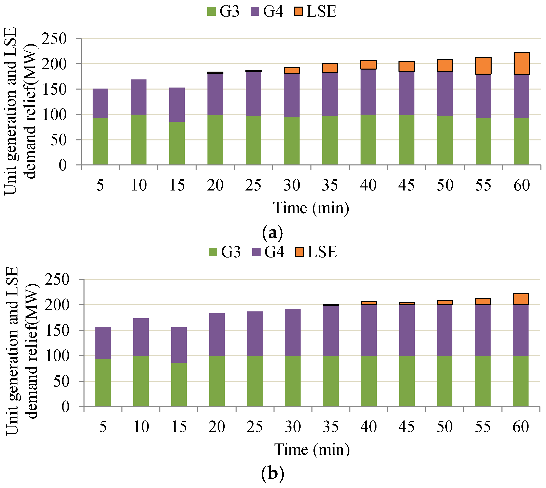
The cost for rewarding LSEs is given as

$$c^{\mathrm{reward}}={\displaystyle \sum _{j\in J}{\lambda }^{\mathrm{CAP}}{L}_j^{\mathrm{IL},\max }}+{\displaystyle \sum _{s\in S}\frac{\Delta t}{60}}{\rho }_s{\displaystyle \sum _{t\in T}{\displaystyle \sum _{j\in J}({\lambda }_j^{\mathrm{DR}}\Delta L_{j,t,s}^{\mathrm{IL}}+{\lambda }^{\mathrm{FRP}}{R}_{j,t,s}^{\mathrm{FRP}})}}$$

(3)

In (3), J is the set of all LSEs with index j. λ^CAP is the compensation to LSEs for providing demand-side resource, which is similar to operating reserve and can provide additional capacity (i.e., $L_j^{\mathrm{IL},\max }$) in the event that units have to reduce their output or be taken offline. ${\lambda }_j^{\mathrm{DR}}$ is the reward to LSE j for providing unit demand relief and is negotiated by the ISO and LSE j in their specific IL contract, and Δ$L_{j,t,s}^{\mathrm{IL}}$ is the amount of demand relief provided by LSE j in period t under scenario s. λ^FRP is the system-level demand price of FRP set by the ISO, and $R_{j,t,s}^{\mathrm{FRP}}$ is the awarded upward FRP capacity of LSE j in period t under scenario s. The main difference between demand relief and FRP is that demand relief is the realized load shedding, while FRP is the deductible capability reserved for the next interval.

c^penalty is composed of the cost for base-load shedding and RES output curtailment penalty, and described by

$$c^{\mathrm{penalty}}={\displaystyle \sum _{s\in S}\frac{\Delta t}{60}}{\rho }_s(\nu {\displaystyle \sum _{t\in T}\Delta L_{t,s}^{\mathrm{BL}}}+\phi {\displaystyle \sum _{t\in T}{\displaystyle \sum _{w\in W}{D}_{w,t,s}}})$$

(4)

where ν is the value of lost base load, Δ$L_{t,s}^{\mathrm{BL}}$ is the amount of lost base load in period t under scenario s. φ is the penalty for unit RES output curtailment, D_w,t,s is the amount of curtailed output of RES w in period t under scenario s.

The objective function in (1) is subject to general UC constraints and FRP-related constraints. The general UC constraints include unit ramping up/down limits, unit generation limits, the maximum limits on base load shedding and RES output curtailment, and power balance constraint [5,25]. The FRP-related constraints reflect the system-wide ramp capability requirement, the impacts of FRP on unit generation and the maximum limits on interruptible load shedding. All constraints are categorized and listed as follows:

• Output bounds of generating units

  $$P_{g,t,s}+R_{g,t,s}^{\mathrm{UP}}\le x_{g,t}{P}_g^{\max }\forall g\in G,\forall t\in T,\forall s\in S$$

  (5)

  $$P_{g,t,s}-R_{g,t,s}^{\mathrm{DN}}\le x_{g,t}{P}_g^{\min }\forall g\in G,\forall t\in T,\forall s\in S$$

  (6)
• Ramping limits of generating units

  $$P_{g,t,s}-P_{g,t-1,s}\le r_g^{\mathrm{UP}}\Delta t\forall g\in G,\forall t\in T,\forall s\in S$$

  (7)

  $$-P_{g,t,s}+P_{g,t-1,s}\le r_g^{\mathrm{DN}}\Delta t\forall g\in G,\forall t\in T,\forall s\in S$$

  (8)

  $$R_{g,t,s}^{\mathrm{UP}}\le r_g^{\mathrm{UP}}\Delta t\forall g\in G,\forall t\in T,\forall s\in S$$

  (9)

  $$R_{g,t,s}^{\mathrm{DN}}\le r_g^{\mathrm{DN}}\Delta t\forall g\in G,\forall t\in T,\forall s\in S$$

  (10)
• Limits on base-load shedding and RES output curtailment

  $$\Delta L_{t,s}^{\mathrm{BL}}\le L_{t,s}^{\mathrm{BL}}\forall t\in T,\forall s\in S$$

  (11)

  $$D_{w,t,s}\le P_{w,t,s}\forall w\in W,\forall t\in T,\forall s\in S$$

  (12)
• Limits on IL capacity

  $$\Delta L_{j,t,s}^{\mathrm{IL}}+R_{j,t,s}^{\mathrm{FRP}}\le L_j^{\mathrm{IL},\max }\forall j\in J,\forall t\in T,\forall s\in S$$

  (13)
• Power balance and ramp capability requirement

  $${\displaystyle \sum _{g\in G}{P}_{g,t,s}}+{\displaystyle \sum _{w\in W}{P}_{w,t,s}}+{\displaystyle \sum _{j\in J}\Delta L_{j,t,s}^{\mathrm{IL}}}+\Delta L_{t,s}^{\mathrm{BL}}=L_{t,s}^{\mathrm{BL}}+{\displaystyle \sum _{j\in J}{L}_j^{\mathrm{IL},\max }}+{\displaystyle \sum _{w\in W}{D}_{w,t,s}}\forall t\in T,\forall s\in S$$

  (14)

  $${\displaystyle \sum _{g\in G}{R}_{g,t,s}^{\mathrm{UP}}}+{\displaystyle \sum _{j\in J}{R}_{j,t,s}^{\mathrm{FRP}}}\ge \Delta L_{t,s}^{\mathrm{NL}}+{\varphi }_{t,s}^{\mathrm{UP}}\forall t\in T,\forall s\in S$$

  (15)

  $${\displaystyle \sum _{g\in G}{R}_{g,t,s}^{\mathrm{DN}}}\ge -\Delta L_{t,s}^{\mathrm{NL}}+{\varphi }_{t,s}^{\mathrm{DN}}\forall t\in T,\forall s\in S$$

  (16)

  $$P_{g,t,s},\Delta L_{j,t,s}^{\mathrm{IL}},R_{j,t,s}^{\mathrm{FRP}},\Delta L_{t,s}^{\mathrm{BL}},D_{w,t,s},R_{g,t,s}^{\mathrm{UP}},R_{g,t,s}^{\mathrm{DN}}\ge 0$$

  (17)

Constraints (5) and (6) enforce the output bounds of units where $P_g^{\max }$ ($P_g^{\min }$) is the maximum (minimum) output of unit g, x_g,t is the on/off state variable of unit g, and $R_{g,t,s}^{\mathrm{UP}}$ ($R_{g,t,s}^{\mathrm{DN}}$) is the upward (downward) FRP provided by unit g in period t under scenario s. It is notable that since the FRP is the focus of this work, provisions of other services (e.g., regulation and operating reserve) are not considered for simplicity. Constraints (7) and (8) restrict the change in the output of units between two contiguous time periods within their maximum ramp capabilities. Note that $r_g^{\mathrm{UP}}$ ($r_g^{\mathrm{DN}}$) is the upward (downward) ramping rate of unit g. Constraints (9) and (10) ensure that a unit’s provision of FRP does not exceed its ramp capability over the dispatching interval.

The amount of acceptable base-load shedding is capped with constraint (11) where $L_{t,s}^{\mathrm{BL}}$ is the base load without shedding. Similar rationale applies for RES output curtailment as shown in constraint (12), in which P_w,t,s is the RES output without curtailment. In terms of IL, Constraint (13) imposes that a LES’s total provision of demand relief and FRP should not exceed its overall capacity.

Constraint (14) enforces the system generation-demand power balance. Constraints (15) and (16) define the system-level ramp capability requirements which are composed of the forecasted net load variability (Δ$L_{t,s}^{\mathrm{NL}}$) and additional uncertainty. The magnitude of surrounding uncertainty (${\varphi }_{t,s}^{\mathrm{UP}}$ and ${\varphi }_{t,s}^{\mathrm{DN}}$), as explained in Section 2.2, can be constant based on the system scale [26] or is the function of forecasted load and RES output [5]. Finally, constraint (17) points out the positive variables.

3. Designing Incentive Compatible Contracts between a LSE and Its Customers

3.1. LSE’s IL Relief Model

Consider a LSE who manages I interruptible customers with different cost-quantity characteristics. The LSE’s role is to allocate its deployed services, namely FRP and demand relief, between different customers and meanwhile to minimize the overall cost of all customers to curtail their loads. The objective function is expressed as:

$$\min {\displaystyle \sum _{i\in I}{C}_i(x_i,{\theta }_i)}$$

(18)

$$C_i(x_i,{\theta }_i)=a^{\mathrm{IL}}{x}_i^2+b^{\mathrm{IL}}{\theta }_i{x}_i$$

(19)

where C_i(x_i, θ_i) is the outage cost function of customer i [12], the variable x_i is the amount of demand relief, the coefficients a^IL and b^IL are the IL cost coefficients [12], and θ_i is the parameter used to sort the customers from the most willing to the least willing to shed load. θ_i indicates customer type and is normalized to be in the range [0, 1] [10].

The associated constraints are listed as follows:

$${\displaystyle \sum _{i\in I}{x}_i}=D$$

(20)

$$x_i\le x_i^{\max }\forall i\in I$$

(21)

where D is the total required demand relief for the LSE, and $x_i^{\max }$ is the maximum amount of demand relief that customer i can provide.

3.2. Incentive Compensation to the Customers

In electricity markets, the true value of θ_i is unknown to the LSE as the customer’s confidential information. However, the customer will have submitted different θ_i in previous contracts and thus the LSE has the relevant historical θ_i to estimate the probability distribution. Based on this historical data, incentive compatible contracts are designed in this work so that rational customers who wish to maximize their own profits are encouraged to reveal their true customer type.

The LSE is assumed to reward customer i based on its submitted customer type ${\theta }_i^{\mathrm{S}}$:

$$A_i(x_i({\theta }_i^{\mathrm{S}}),{\theta }_i^{\mathrm{S}})=C_i(x_i({\theta }_i^{\mathrm{S}}),{\theta }_i^{\mathrm{S}})+B_i({\theta }_i^{\mathrm{S}})$$

(22)

where A_i is the reward which consists of the demand relief payment C_i defined in (19) and extra incentive compensation B_i related to ${\theta }_i^{\mathrm{S}}$. x_i(${\theta }_i^{\mathrm{S}}$) is the amount of demand relief assigned to customer i after the LSE runs the IL relief model. x_i(${\theta }_i^{\mathrm{S}}$) is associated with customer types submitted by both customer i and all the other customers. It is assumed that for each customer, its possible submitted customer type is subject to a specific statistical distribution with bounds [${\theta }_i^{\min }$, ${\theta }_i^{\max }$], which is known by the LSE from existing historical utility data. Therefore, Monte Carlo (MC) simulations can be performed to model the customers’ behaviors. Afterwards, the expected profit of customer i can be calculated as the received reward minus the true outage cost:

$$P_i({\theta }_i^{\mathrm{S}},{\theta }_i^{\mathrm{T}})=A_i(x_i^{\exp }({\theta }_i^{\mathrm{S}}),{\theta }_i^{\mathrm{S}})-C_i(x_i^{\exp }({\theta }_i^{\mathrm{S}}),{\theta }_i^{\mathrm{T}})=\underset{\mathrm{strategically}\mathrm{bidding}\mathrm{revenue}}{\underbrace{b^{\mathrm{IL}}({\theta }_i^{\mathrm{S}}-{\theta }_i^{\mathrm{T}})x_i^{\exp }({\theta }_i^{\mathrm{S}})}}+\underset{\mathrm{incentive}\mathrm{compensation}}{\underbrace{B_i({\theta }_i^{\mathrm{S}})}}$$

(23)

where ${\theta }_i^{\mathrm{T}}$ is the true customer type of customer i, and $x_i^{\exp }$(${\theta }_i^{\mathrm{S}}$) is the expected amount of demand relief over all MC simulations. The first part of the expected profit is the strategically bidding revenue. Customer i may intend to submit a large ${\theta }_i^{\mathrm{S}}$ in order to obtain higher revenue if no incentive compensation is in place.

Incentive compatible principle requires that customer i obtains the highest expected profit if the customer submits its true customer type, which can be mathematically formulated as the partial derivative of the expected profit function with respect to the submitted customer type ${\theta }_i^{\mathrm{S}}$ is equal to zero:

$$\frac{\partial P_i({\theta }_i^{\mathrm{S}},{\theta }_i^{\mathrm{T}})}{\partial {\theta }_i^{\mathrm{S}}}={\left[b^{\mathrm{IL}}({\theta }_i^{\mathrm{S}}-{\theta }_i^{\mathrm{T}}){(x_i^{\exp }({\theta }_i^{\mathrm{S}}))}^{\prime }+b^{\mathrm{IL}}{x}_i^{\exp }({\theta }_i^{\mathrm{S}})+B_i^{\prime }({\theta }_i^{\mathrm{S}})\right]|}_{{\theta }_i^{\mathrm{S}}={\theta }_i^{\mathrm{T}}}=0$$

(24)

The first item b^IL(${\theta }_i^{\mathrm{S}}$ − ${\theta }_i^{\mathrm{T}}$)($x_i^{\exp }$(${\theta }_i^{\mathrm{S}}$))’ is equal to zero if ${\theta }_i^{\mathrm{S}}$ = ${\theta }_i^{\mathrm{T}}$, thus (24) can be simplified as

$$B_i^{\prime }({\theta }_i^{\mathrm{S}})=-b^{\mathrm{IL}}{x}_i^{\exp }({\theta }_i^{\mathrm{S}})$$

(25)

After integrating both sides of (25) over the interval [${\theta }_i^{\mathrm{S}}$, ${\theta }_i^{\max }$] and setting B_i(${\theta }_i^{\max }$) = 0, the incentive compensation to customer i can be expressed as:

$$B_i({\theta }_i^{\mathrm{S}})=b^{\mathrm{IL}}{\displaystyle {\int }_{{\theta }_i^{\mathrm{S}}}^{{\theta }_i^{\max }}{x}_i^{\exp }({\theta }_i^{\mathrm{S}})}d{\theta }_i^{\mathrm{S}}$$

(26)

The demand relief allocated to a customer is greater than or equal to zero and monotonically decreasing with the submitted customer type. This is because a large customer type indicates a costly outage, thus this customer will be an unfavorable choice to provide demand relief. Figure 3 shows how expected demand relief normally changes with submitted customer type. b^IL is assumed to be 1 for illustration purposes. As observed, the incentive compensation a customer receives is closely related to its submitted customer type. A small submitted customer type will increase the compensation (the area of the shaded part in Figure 3), and vice versa.

On the other hand, a small submitted customer type will decrease the strategically bidding revenue, as shown in (23). Incentive compatible ensures the customer gains the highest expected profit by submitting its true customer type ${\theta }_i^{\mathrm{T}}$. If the customer submits a different ${\theta }_i^{\mathrm{d}}$, the difference in expected profit is calculated as:

$$\begin{array}{cc}\hfill \Delta P_i& =P_i({\theta }_i^{\mathrm{d}},{\theta }_i^{\mathrm{T}})-P_i({\theta }_i^{\mathrm{T}},{\theta }_i^{\mathrm{T}})\hfill \\ & =b^{\mathrm{IL}}({\theta }_i^{\mathrm{d}}-{\theta }_i^{\mathrm{T}})x_i^{\exp }({\theta }_i^{\mathrm{d}})+b^{\mathrm{IL}}{\displaystyle {\int }_{{\theta }_i^{\mathrm{d}}}^{{\theta }_i^{\max }}{x}_i^{\exp }({\theta }_i^{\mathrm{S}})}d{\theta }_i^{\mathrm{S}}-b^{\mathrm{IL}}{\displaystyle {\int }_{{\theta }_i^{\mathrm{T}}}^{{\theta }_i^{\max }}{x}_i^{\exp }({\theta }_i^{\mathrm{S}})}d{\theta }_i^{\mathrm{S}}\hfill \\ & =b^{\mathrm{IL}}({\theta }_i^{\mathrm{d}}-{\theta }_i^{\mathrm{T}})x_i^{\exp }({\theta }_i^{\mathrm{d}})-b^{\mathrm{IL}}{\displaystyle {\int }_{{\theta }_i^{\mathrm{T}}}^{{\theta }_i^{\mathrm{d}}}{x}_i^{\exp }({\theta }_i^{\mathrm{S}})}d{\theta }_i^{\mathrm{S}}\hfill \end{array}$$

(27)

(27) is transformed by using the Lagrange Mean Value Theorem:

$$\Delta P_i=b^{\mathrm{IL}}({\theta }_i^{\mathrm{d}}-{\theta }_i^{\mathrm{T}})(x_i^{\exp }({\theta }_i^{\mathrm{d}})-x_i^{\exp }(\epsilon ))$$

(28)

where ε is between ${\theta }_i^{\mathrm{d}}$ and ${\theta }_i^{\mathrm{T}}$; if ${\theta }_i^{\mathrm{d}}$ > ${\theta }_i^{\mathrm{T}}$, there is $x_i^{\exp }$(${\theta }_i^{\mathrm{d}}$) ≤ $x_i^{\exp }$(ε) due to the decreasing property of $x_i^{\exp }$(${\theta }_i^{\mathrm{S}}$) and thus ΔP_i ≤ 0; the same result can be obtained if ${\theta }_i^{\mathrm{d}}$ < ${\theta }_i^{\mathrm{T}}$. Therefore, submitting a customer type different from the true value will generate no additional expected profit and thus, it is in the customer’s best interest to reveal the true outage cost in order to collect the highest profit.

3.3. Calculating the LSE’s Profit

The expected demand relief Δ$L_{j,t}^{\mathrm{IL},\exp }$ and FRP $R_{j,t}^{\mathrm{FRP},\exp }$ in the time period t provided by LSE j over all scenarios are solved as the outputs of the stochastic RTUC model and are calculated as:

$$\Delta L_{j,t}^{\mathrm{IL},\exp }={\displaystyle \sum _{s\in S}{\rho }_s\Delta L_{j,t,s}^{\mathrm{IL}}}$$

(29)

$$R_{j,t}^{\mathrm{FRP},\exp }={\displaystyle \sum _{s\in S}{\rho }_s{R}_{j,t,s}^{\mathrm{FRP}}}$$

(30)

For each independent time period t ∈ T, LSE j runs the IL relief model considering Δ$L_{j,t}^{\mathrm{IL},\exp }$ and $R_{j,t}^{\mathrm{FRP},\exp }$ as inputs. Results include FRP and demand relief provision of each customer and their respective payments. It is assumed that $R_{j,t}^{\mathrm{FRP},\exp }$ is allocated among all the customers in a pro-rated manner and thus reduces the maximum amount of demand relief the customer can provide. In other words, the customers are required to leave a margin for FRP and therefore unable to curtail all their loads.

Additionally, all the customers are expected to submit their true customer types due to the incentive compensation. Hence, the expected profit of LSE j over all time periods is equal to the reward from the ISO minus the payment to its customers:

$${\pi }_j={\lambda }^{\mathrm{CAP}}{L}_j^{\mathrm{IL},\max }+{\displaystyle \sum _{s\in S}\frac{\Delta t}{60}}{\rho }_s{\displaystyle \sum _{t\in T}({\lambda }_j^{\mathrm{DR}}\Delta L_{j,t,s}^{\mathrm{IL}}+{\lambda }^{\mathrm{FRP}}{R}_{j,t,s}^{\mathrm{FRP}})}-{\displaystyle \sum _{t\in T}\frac{\Delta t}{60}{\displaystyle \sum _{i\in I}{A}_i(x_i({\theta }_i^{\mathrm{T}}),{\theta }_i^{\mathrm{T}})}}$$

(31)

The LSE is happy if π_j is no less than its acceptable minimum profit ${\pi }_j^{\min }$. Otherwise, it might request for a higher reward to provide demand-side services for the ISO.

4. Solving Process

The flowchart for solving the proposed work is presented in Figure 4. The whole process is terminated only when the LSE is properly rewarded. Otherwise, the LSE will stop providing services or ask for a higher reward from the ISO. Note the settlement of ${\lambda }_j^{\mathrm{DR}}$ is not real-time scale and might need a long-term negotiation between the LSE and the ISO. The ultimate goal is incorporating a proper reward mechanism which allows both parties to be profitable. The negotiation process, however, entails more detailed study and is beyond the scope of this work. Instead, this work endeavours to prove that with proper reward mechanisms, not only the ISO, but also the LSE can benefit in IL simultaneous provision of FRP and demand relief.

5. Case Studies and Numerical Results

A power system including five generating units, one RES and one LSE is employed to demonstrate the performance of the proposed method. The characteristics of units (

Table 2. Characteristics of generating units.

Unit	${\mathit{P}}_{\mathit{g}}^{\mathbf{m}\mathbf{a}\mathbf{x}}$ (MW)	${\mathit{P}}_{\mathit{g}}^{\mathbf{m}\mathbf{i}\mathbf{n}}$ (MW)	${\mathit{r}}_{\mathit{g}}^{\mathbf{U}\mathbf{P}}$ (MW/min)	${\mathit{r}}_{\mathit{g}}^{\mathbf{D}\mathbf{N}}$ (MW/min)	${\mathit{P}}_{\mathit{g}}^{\mathbf{i}\mathbf{n}\mathbf{i}\mathbf{t}}$ (MW)	ag ($/h)	bg ($/MWh)	${\mathit{c}}_{\mathit{g}}^{\mathbf{S}\mathbf{U}}$ ($)
G1	280	280	0	0	280	0	5	0
G2	150	50	2.8	2.8	120	200	10	300
G3	100	30	2.8	2.8	80	200	20	600
G4	100	20	2.8	2.8	60	200	30	900
G5	100	5	6	6	0	300	50	1200

) are modified based on [27]. The overall operation cost of unit g is assumed to be a linear function of its output: C_g(P_g) = a_g + b_gP_g [5]. Among these units, G1 is a base-load unit with zero ramp rate and least operation cost, while G5 is a fast-starting unit with the highest operation cost and fastest ramp rate. G2–G4 are regular units with operation and start-up costs in between. The RES output is regarded as the aggregation of the outputs from multiple RESs. The LSE manages three customers whose maximum ILs and type parameters are given in

Table 3. Parameters of interruptible loads.

Customer	Maximum IL (MW)	True Type Parameter ${\mathit{\theta }}_{\mathit{i}}^{\mathbf{T}}$	Low Bound of Type Parameter ${\mathit{\theta }}_{\mathit{i}}^{\mathbf{m}\mathbf{i}\mathbf{n}}$	High Bound of Type Parameter ${\mathit{\theta }}_{\mathit{i}}^{\mathbf{m}\mathbf{a}\mathbf{x}}$
1	10	0.32	0.26	0.4
2	20	0.44	0.35	0.52
3	30	0.52	0.46	0.6

. Customer 1, 2 and 3 are ranked from the most willing to provide demand relief to the least willing. For the respective customer type i (i = 1, 2, 3), it is estimated by the LSE to follow the continuous uniform distribution with minimum value ${\theta }_i^{\min }$ and maximum value ${\theta }_i^{\max }$. The cost coefficients of IL are set as a^IL = 1 $/MW²h, b^IL = 120 $/MWh [12].

The clearing granularity of RTUC is set as 5 min in line with the current market practice [1,2]. Figure 5 presents the 5-min forecasted base load and RES output during a typical peak hour. The forecasted net load is also presented in Figure 5, defined as the difference between the forecasted base load and the RES output plus the total amount of ILs (60 MW in this case study). As observed, the net load profile is variable and fluctuant. On one hand, the general upward tendency represents the upward variability, which calls for the IL customers to curtail their loads in order to maintain the balance between power supply and demand. On the other hand, the decline in the time interval from the 10th min to the 15th min represents the fluctuation of the net load.

The base load and RES output are both assumed to follow normal distributions with the standard deviations of the base load and RES output being 1% and 10% of the expected values, respectively [25]. Three thousand scenarios for base load are generated by using the Latin hypercube sampling method [22] and 10 representative scenarios are selected based on the fast forward selection algorithm [23]. The probability of each selected scenario is also obtained from the fast forward selection. Similar process applies for the RES output to obtain 10 representative RES generation scenarios. Finally, 100 combined scenarios with the specified load $L_{t,s}^{\mathrm{BL}}$ and RES output $P_{t,s}^{\mathrm{W}}$ chosen from the above load scenarios and RES output scenarios are obtained, as well as their corresponding conditional probabilities. Based on these system-level forecasts, the underlying uncertainties in scenario s can be formulated in a linear form [5]:

$${\varphi }_{t,s}^{\mathrm{UP}}={\alpha }^{\mathrm{l},\mathrm{up}}{L}_{t+1,s}^{\mathrm{BL}}+{\beta }^{\mathrm{l},\mathrm{up}}{P}_{t+1,s}^{\mathrm{W}}$$

(32)

$${\varphi }_{t,s}^{\mathrm{DN}}={\alpha }^{\mathrm{l},\mathrm{dn}}{L}_{t+1,s}^{\mathrm{BL}}+{\beta }^{\mathrm{l},\mathrm{dn}}{P}_{t+1,s}^{\mathrm{W}}$$

(33)

In practice, the value of the coefficients can be tuned according to the forecast accuracy and in this study is set as α^l,up = α^l,dn = 0.01 and β^l,up = β^l,dn = 0.05. Note that β is larger than α because the RES output is normally more variable than the system load. Moreover, sensitivity analysis will be conducted on β in order to show the impacts of the RES output uncertainty and how IL can effectively assist in uncertainty mitigation.

Additionally, specify ν = 3500 $/MWh and φ = 50 $/MWh [28]. λ^CAP is set to 1.35 $/MW, which is close to the price of operating reserve in MISO [29]. λ^FRP is set to 5 $/MWh following MISO’s practice [2]. λ^DR is assumed to be 50 $/MWh set forth by the ISO in the beginning and might be raised according to the results of the profit calculation, which terminates the whole process if the LSE’s yield rate is over 25%.

Two highly efficient optimizers are employed to solve the presented model. The stochastic RTUC model is implemented in GAMS [30] as a mixed-integer linear program (MILP) and solved by CPLEX, and the IL relief model is solved in MATLAB as a quadratic programming problem.

5.1. LSE’s Provision of FRP and Demand Relief

To demonstrate the role of the LSE in maintaining the system generation-demand power balance and reducing the operation cost, three cases are considered as follows:

• Case 1: the LSE is treated as inelastic load and neither demand nor FRP are called upon;
• Case 2: the LSE is only allowed to provide demand relief;
• Case 3: the LSE can provide both FRP and demand relief.

Table 4. Summary of unit commitment results for different cases.

Case	Total Cost ($)	Total Cost Reduction	Unit Generation Cost ($)	Rewards to the LSE ($)	G5 Running Time (min)
1	9991.5	0%	9910.5	81	60
2	9954.2	0.37% *	9156.4	797.8	15
3	8487.6	15.05% *	8119.3	369.3	0

* The ratio is calculated based on the total cost in Case 1.

summarizes the expected results over all scenarios for three cases. In Case 1, without supports from the LSE, the ISO has to start G5 at the first time interval and keeps it ON at all times in order to keep power balance and to meet the ramp capability requirement, which results in the highest generation cost of all cases. Taking advantage of the LSE provision of demand relief in Case 2, the generation cost reduces since the expensive production of unit G5 is reduced. However, an extra cost is incurred to reward the LSE for demand relief and thus results in a very limited reduction (0.37%) in total cost when compared with Case 1. A significant cost deduction (15.05%) is seen in Case 3, which is because the commitment of G5 is avoided, and meanwhile, the rewards to the LSE decrease as less demand relief is called upon. This occurs because the LSE provides cost-effective FRP using IL and thus forces unit G5 to be extra-marginal.

To analyze the impacts of introducing the LSE as a FRP provider, detailed comparisons are drawn between Case 2 and Case 3. Figure 6 presents the average portfolio of FRP provisions in the two cases. Note that in the period t₂, the upward ramp capability requirement is zero because there is a distinct decrease in net load and no upward FRP is needed. In Figure 6, it is shown the LSE can replace the expensive unit G5 by providing upward FRP, especially when the requirement is high (e.g., in t₁ and t₃). In this way, the undesirable startup cost and generation cost is avoided. Furthermore, with the LSE’s participation, units G3 and G4 are released from limitations of upward FRP provision and thus can provide their energy to maintain system balance, which in turn leads to less demand relief requirement from the LSE. This process is shown in Figure 7, which only presents the results of G3, G4 and LSE for purposes of clarity. The results of G1 and G2, as base-load units, are not presented for negligible distinctions in Case 2 and Case 3. It should be pointed out that in Case 2, G5 is cycled from the onset and keeps generating at its minimum output for the first three time intervals in order to provide upward FRP. This is inefficient and not cost-effective.

In situations where the RES output is more volatile, the associated uncertainty increases, rendering a larger β and consequently higher ramp capability requirements.

Table 5. FRP provision with the increasingly volatile RES output.

β	Total Required FRP (MW)	Upward FRP by the LSE (MW)	Upward FRP by the Units (MW)	G5 Running Time (min)	G5 Output (MW)
0.05	230.3	131.6	98.7	0	0
0.10	277.4	177.5	99.9	0	0
0.15	325.5	225.6	99.9	0	0
0.20	378.7	273	105.7	5	5

summarizes the results of different scenarios with varying β. As β increases in the range of [0.05, 0.15], the total required upward FRP over all time intervals increases, which is then met by the provision of the LSE and conventional units. The former increases its provision according to the system requirement, whereas the latter keeps its provision almost constant. This is the case because units G1–G4 can only provide limited amount of FRP due to their ramp rate and maximum power constraints. When β increases to 0.2, the ISO must cycle G5 in t₃ to provide sufficient FRP to meet the higher ramp capability requirement caused by the RES output uncertainty. This undesirable deployment of G5 might occur more frequently in systems with significant penetration of RES. Based on the above analysis, therefore, exploring more ILs is beneficial for reducing the frequency of deploying costly units.

5.2. Incentive Compensation to the Customers

After the system operator runs the stochastic RTUC model, the expected demand relief Δ$L_{j,t}^{\mathrm{IL},\exp }$ and FRP $R_{j,t}^{\mathrm{FRP},\exp }$ in time period t provided by LSE j over all scenarios are solved and presented in

Table 6. Expected FRP and demand relief provided by the LSE.

t	Time (min)	Δ${\mathit{L}}_{\mathit{t}}^{\mathbf{I}\mathbf{L}\mathbf{,}\mathbf{e}\mathbf{x}\mathbf{p}}$ (MW)	${\mathit{R}}_{\mathit{t}}^{\mathbf{F}\mathbf{R}\mathbf{P}\mathbf{,}\mathbf{e}\mathbf{x}\mathbf{p}}$ (MW)
1	5	0	7.32
2	10	0	0
3	15	0	10.41
4	20	0	1.18
5	25	0	3.33
6	30	0	11.25
7	35	1.01	16.07
8	40	6.05	10.15
9	45	5.11	14.97
10	50	8.83	15.51
11	55	13.05	20.37
12	60	21.99	21.06

. The LSE starts to provide demand relief at t₇ and onwards. On the other hand, the LSE is required to provide FRP in all time periods except t₂. The required capacity, as already mentioned, is assigned within all customers using a pro-rated method in proportion to their maximum IL.

To validate the effectiveness of the designed incentive compensation, for each customer in each individual time period t (t = 7, 8, ..., 12), the expected amount of demand relief $x_i^{\exp }$(${\theta }_i^{\mathrm{S}}$) is calculated with varying submitted customer type ${\theta }_i^{\mathrm{S}}$. The other customers’ behaviours are modelled by MC simulation. Note that a larger number of MC trials provides more precise results, but introduces higher computational burden. A trade-off is achieved by setting the number of MC trials to 1000 in this study, which averages a 1-min computation time to obtain results for each customer.

The results for each customer are shown in Figure 8. As observed, for all the customers, the expected amount of demand relief decreases as the submitted customer type increases. It is noteworthy that for Customer 1, the expected amount of demand relief almost remains constant in t₁₁ and t₁₂. This is because Customer 1 is most willing to curtail load and thus is given priority. Particularly in t₁₂ when the requirement for demand relief is high, all available capacity of Customer 1 is deployed regardless of its submitted customer type. In contrast, as the least willing to curtail load, Customer 3 is seldom deployed in time periods t₇, t₈ and t₉ when the requirement for demand relief is low.

The expected profits of the customers, as defined in (23), are presented in Figure 9, which also shows the two revenue streams (i.e., the strategically bidding revenue and the incentive compensation). Note that all customers’ profits in each individual time period are calculated but only a typical subset (t₁₂) is shown for illustration.

Figure 9 shows that a customer who intentionally submits a higher customer type will receive more revenues from bidding, but meanwhile is awarded less compensation. These two opposite effects offset each other and keep the expected profit of Customer 1 constant, as Figure 9a shows. Customer 1 is always got fully deployed in t₁₂, as shown in Figure 8a. Therefore, it can be proved by (23) and (26) that customer 1 is expected to receive same profit, which is also the maximum profit it can obtain. In contrast, as shown in Figure 9b,c, it is in the best interest for Customer 2 and 3 to submit their true customer types. It is noticeable that even though the increase in the expected profit is insignificant, it is only the profit over the 5-min time interval and would be mirrored as significant monies over long periods.

5.3. Calculating the LSE’s Profit

After all customers submit their true customer types, the LSE runs the IL relief model and calculates the total reimbursement to its customers which consists of the demand relief payment and the incentive compensation. The results for each time period are shown in

Table 7. Reimbursement from the LSE to its customers.

t	1–6	7	8	9	10	11	12	Total
demand relief payment	0	3.3	22.4	18.5	34.7	56.5	107.7	243.2
incentive compensation	0	0.7	4.0	3.4	6.	9.3	15.9	39.4
Total reimbursement	0	4.0	26.4	21.9	40.7	65.8	123.6	282.6

. The LSE’s own profit, which is equal to the reward from the ISO ($369.3 as shown in Table 4) minus the reimbursement to the customers ($282.6), is $86.7, rendering a yield rate of 30.7%. This indicates the LSE is well paid under the existing price mechanism and is willing to provide services.

6. Conclusions

With the ever-growing penetration of RESs in power systems, FRP has become a new market product for addressing the challenges in power system operation. The basic concept and technical characteristics of FRP are introduced, and FRP imposes much less technical requirement for potential providers than other ancillary services. Subsequently, the mechanism of simultaneous provision of FRP and demand relief by IL is explored. The LSE is introduced as the mediator between multiple IL customers and the ISO. A stochastic RTUC model considering ramp requirements and IL participation is then presented to formulate the interactions between the ISO and LSEs. Simulation results show that the overall system benefits with LSEs as service providers come from three major aspects: (1) the start-up and operation costs of expensive units are avoided; (2) through provision of FRP by ILs, generating units are released, at least to some extent, from the requirement of upward FRP and thus can allocate generation resources to other needs of the power system; and (3) there is more flexibility for the power system concerned to meet the increased ramp requirement caused by high penetration of RES. On the other hand, the LSEs can also benefit by providing these services if proper compensations are in place.

The interactions between LSEs and their customers are simulated using economic incentives. As a profit-seeking entity, each LSE runs a IL relief model, aiming to minimize the overall outage cost of its managed IL customers. On the other hand, IL customers intend to attain more profit by strategically reporting their customer types. To this end, an incentive compatible mechanism is designed so as to encourage each LSE to collect information about its customers. Simulation results show that customers with different cost-quantity characteristics are encouraged to reveal their true outage costs so as to gain the highest profits.

This work also discusses the mechanism and possibility of including IL as a FRP provider. A case study is employed to demonstrate the feasibility of the proposed method. Technical details of different kinds of RESs are not presented in this paper due to space limitation. It will be our future research effort to extend this study to actual power systems with targeted RES penetration levels so as to investigate the practical feasibility and to attain quantitative benefits with the participation of ILs.

References

1. California Independent System Operator (CAISO). Flexible Ramping Product. 2012. Available online: http://www.caiso.com/documents/draftfinalproposal-flexiblerampingproduct.pdf (accessed on 10 April 2012).
2. Midcontinent Independent System Operator (MISO). Ramp Capability Product Design for MISO Markets. 2013. Available online: https://www.misoenergy.org/Library/Repository/Communication%20Material/Key%20Presentations%20and%20Whitepapers/Ramp%20Product%20Conceptual%20Design%20Whitepaper.pdf (accessed on 10 July 2013).
3. Cornelius, A. Assessing the Impact of Flexible Ramp Capability Products in the Midcontinent ISO. Ph.D. Dissertation, Duke University, Durham, NC, USA, 2014. [Google Scholar]
4. California Independent System Operator (CAISO). What the Duck Curve Tells Us about Managing a Green Grid. 2016. Available online: https://www.caiso.com/Documents/FlexibleResourcesHelpRenewables_FastFacts.pdf (accessed on 8 September 2016).
5. Chen, R.; Wang, J.; Botterud, A.; Sun, H. Wind power providing flexible ramp product. IEEE Trans. Power Syst. 2017, 32, 2049–2061. [Google Scholar] [CrossRef]
6. Cui, M.; Zhang, J.; Wu, H.; Hodge, B.M.; Ke, D.; Sun, Y. Wind power ramping product for increasing power system flexibility. In Proceedings of the 2016 IEEE/PES Transmission and Distribution Conference and Exposition (T&D), Dallas, TX, USA, 3–5 May 2016; pp. 1–5. [Google Scholar]
7. Zhang, B.; Kezunovic, M. Impact on power system flexibility by electric vehicle participation in ramp market. IEEE Trans. Smart Grid 2016, 7, 1285–1294. [Google Scholar] [CrossRef]
8. Tuan, L.A.; Bhattacharya, K. Competitive framework for procurement of interruptible load services. IEEE Trans. Power Syst. 2000, 15, 889–897. [Google Scholar]
9. Zhou, X.; Li, W.; Li, M.; Chen, Q.; Zhang, C.; Yu, J. Effect of the coordinative optimization of interruptible loads in primary frequency regulation on frequency recovery. Energies 2016, 9, 167. [Google Scholar] [CrossRef]
10. Fahrioglu, M.; Alvarado, F.L. Designing incentive compatible contracts for effective demand management. IEEE Trans. Power Syst. 2003, 18, 1255–1260. [Google Scholar] [CrossRef]
11. Yu, C.; Zhang, S.; Chung, T.; Wong, K. Modelling and evaluation of interruptible-load programmes in electricity markets. IET Proc. Gen. Transm. Distrib. 2005, 152, 581–588. [Google Scholar] [CrossRef]
12. Li, H.; Li, Y.; Li, Z. A multiperiod energy acquisition model for a distribution company with distributed generation and interruptible load. IEEE Trans. Power Syst. 2007, 22, 588–596. [Google Scholar] [CrossRef]
13. Fahrioglu, M.; Alvarado, F.L. Using utility information to calibrate customer demand management behavior models. IEEE Trans. Power Syst. 2001, 16, 317–322. [Google Scholar] [CrossRef]
14. US Department of Energy. Benefit of Demand Response in Electricity Markets and Recommendations for Achieving Them: A Report to the United State Congress Pursuant to Section 1252 of the Energy Policy Act of 2005. Available online: http://www.caiso.com/documents/draftfinalproposal-flexiblerampingproduct.pdf (accessed on 1 February 2006).
15. Botterud, A.; Zhou, Z.; Wang, J.; Sumaili, J.; Keko, H.; Mendes, J.; Miranda, V. Demand dispatch and probabilistic wind power forecasting in unit commitment and economic dispatch: A case study of Illinois. IEEE Trans. Sustain. Energy 2013, 4, 250–261. [Google Scholar] [CrossRef]
16. Zhong, H.; Xia, Q.; Xia, Y.; Kang, C.; Xie, L.; He, W.; Zhang, H. Integrated dispatch of generation and load: A pathway towards smart grids. Electr. Power Syst. Res. 2015, 120, 206–213. [Google Scholar] [CrossRef]
17. Park, H.-G.; Lyu, J.-K.; Kang, Y.; Park, J.-K. Unit commitment considering interruptible load for power system operation with wind power. Energies 2014, 7, 4281–4299. [Google Scholar] [CrossRef]
18. Wang, Q.; Hodge, B.M. Enhancing power system operational flexibility with flexible ramping products: A review. IEEE Trans. Ind. Inform. 2017, 13, 1652–1664. [Google Scholar] [CrossRef]
19. Midcontinent Independent System Operator (MISO). Ramp Capability Integration Technical Workshop. 2016. Available online: https://www.misoenergy.org/Library/Repository/Meeting%20Material/Stakeholder/Workshops%20and%20Special%20Meetings/2016/20160115%20Ramp%20Capability%20Integration%20Technical%20Workshop/20160115%20Ramp%20Workshop%20Presentation.pdf (accessed on 15 January 2016).
20. Midcontinent Independent System Operator (MISO). Business Practices Manual 2 (BPM2): Energy and Operating Reserve Markets. 2017. Available online: https://www.misoenergy.org/library/businesspracticesmanuals/Pages/BusinessPracticesManuals.aspx (accessed on 23 September 2017).
21. Morales, J.M.; Pineda, S.; Conejo, A.J.; Carrion, M. Scenario reduction for futures market trading in electricity markets. IEEE Trans. Power Syst. 2009, 24, 878–888. [Google Scholar] [CrossRef]
22. Glasserman, P. Monte Carlo Methods in Financial Engineering; Springer: Heidelberg, Germany, 2003; Volume 53. [Google Scholar]
23. Heitsch, H.; Römisch, W. Scenario reduction algorithms in stochastic programming. Comput. Optim. Appl. 2003, 24, 187–206. [Google Scholar] [CrossRef]
24. Pandzžic, H.; Dvorkin, Y.; Wang, Y.; Qiu, T.; Kirschen, D.S. Effect of time resolution on unit commitment decisions in systems with high wind penetration. In Proceedings of the 2014 IEEE PES General Meeting, Conference & Exposition, National Harbor, MD, USA, 27–31 July 2014; pp. 1–5. [Google Scholar]
25. Wang, J.; Shahidehpour, M.; Li, Z. Security-constrained unit commitment with volatile wind power generation. IEEE Trans. Power Syst. 2008, 23, 1319–1327. [Google Scholar] [CrossRef]
26. Navid, N.; Rosenwald, G. Market solutions for managing ramp flexibility with high penetration of renewable resource. IEEE Trans. Sustain. Energy 2012, 3, 784–790. [Google Scholar] [CrossRef]
27. Wang, B.; Hobbs, B.F. Real-time markets for flexiramp: A stochastic unit commitment-based analysis. IEEE Trans. Power Syst. 2016, 31, 846–860. [Google Scholar] [CrossRef]
28. Park, H.; Baldick, R. Transmission planning under uncertainties of wind and load: Sequential approximation approach. IEEE Trans. Power Syst. 2013, 28, 2395–2402. [Google Scholar] [CrossRef]
29. Argonne National Laboratory (ANL). Survey of U.S. Ancillary Services Markets. Available online: http://www.ipd.anl.gov/anlpubs/2016/01/124217.pdf (accessed on 15 January 2016).
30. General Algebraic Modeling System (GAMS). GAMS—A user’s Guide. Available online: http://www.gams.com/dd/docs/bigdocs/GAMSUsersGuide.pdf (accessed on 15 December 2012).
Figure 1. Maintaining system generation-demand balance by demand relief of interruptible load. (RES output is represented by wind power).
Energies 11 00046 g001
Figure 2. Illustrations of ramp capability requirements and FRP: (a) Multiple time periods; (b) Single time period.
Energies 11 00046 g002
Figure 3. Expected amount of demand relief and incentive compensation versus varying submitted customer type (bIL is assumed to be 1).
Energies 11 00046 g003
Figure 4. Flowchart for solving the proposed model.
Energies 11 00046 g004
Figure 5. Forecasted base load, net load and RES output.
Energies 11 00046 g005
Figure 6. Expected upward FRP provision portfolio in (a) Case 2 and (b) Case 3.
Energies 11 00046 g006
Figure 7. Expected unit generation and LSE demand relief in (a) Case 2 and (b) Case 3.
Energies 11 00046 g007
Figure 8. Expected amount of demand relief of each customer versus varying submitted customer type: (a) Customer 1; (b) Customer 2; (c) Customer 3.
Energies 11 00046 g008
Figure 9. Expected profit of each customer versus varying submitted customer type in t12: (a) Customer 1; (b) Customer 2; (c) Customer 3.
Energies 11 00046 g009aEnergies 11 00046 g009b