Article

A Transient Analytical Model for Predicting Wellbore/Reservoir Temperature and Stresses during Drilling with Fluid Circulation

1
CSIRO Energy, Clayton, VIC 3168, Australia
2
Faculty of Engineering, China University of Geosciences, Wuhan 430074, China
3
SCT Operations, Wollongong, NSW 2500, Australia
4
Department of Civil and Environmental Engineering, University of Pittsburgh, Pittsburgh, PA 15261, USA
5
Department of Chemical and Petroleum Engineering, University of Pittsburgh, Pittsburgh, PA 15261, USA
*
Authors to whom correspondence should be addressed.
Energies 2018, 11(1), 42; https://doi.org/10.3390/en11010042
Submission received: 24 October 2017 / Revised: 23 November 2017 / Accepted: 27 November 2017 / Published: 25 December 2017

Abstract

:
Accurate characterization of heat transfer in a wellbore during drilling, which includes fluid circulation, is important for wellbore stability analysis. In this work, a pseudo-3D model is developed to simultaneously calculate the heat exchange between the flowing fluid and the surrounding media (drill pipe and rock formation) and the in-plane thermoelastic stresses. The cold drilling fluid descends through the drill pipe at constant injection rates and returns to the ground surface via the annulus. The fluid circulation will decrease the wellbore bottom temperature and reduce the near-wellbore high compressive stress, potentially leading to tensile fracturing of the well. The governing equations for the coupled heat transfer stress problem are formulated to ensure that the most important parameters are taken into account. The wellbore is subject to a non-hydrostatic in situ far-field stress field. In modeling heat exchange between fluid and surrounding media, the heat transfer coefficients are dependent on fluid properties and flow behavior. Analytical solutions in the Laplace space are obtained for the temperatures of the fluid in both the drill pipe and annulus and for the temperature and stress changes in the formation. The numerical results in the time domain are obtained by using an efficient inversion approach. In particular, the near-well stresses are compared for the cases with fixed and time-dependent cooling wellbore conditions. This comparison indicates that the using a fixed temperature wellbore conditions may over-estimate or under-estimate the bottom-hole stress change, potentially leading to wellbore stability problems.

1. Introduction

Drilling and completion of wells provides a direct way to extract the resources such as oil, gas and geothermal energy from beneath the earth’s surface. Assessment of the wellbore stability issues is an important but very challenging topic related to safe and efficient drilling operations. Instability of wellbores historically costs the oil and gas industry billions of dollars worldwide annually [1]. During drilling, fluid is circulated through the drill pipe/annulus system and this fluid circulation process serves several fundamental functions: (1) removal of the large amount of drilled cuttings from the wellbore [2]; (2) prevention of breakdown (tensile failure) and breakout (shear failure) of the wellbore by adjusting the mud weight and circulation rate, thus controlling the pressure [3,4]; and (3) cooling and lubricating of the drill bit [5]. In addition, the heat exchange between drilling fluids and surrounding formation results in thermoelastic stress redistribution near the wellbore.
Wellbore stability is affected by a variety of factors, such as mechanical impact as a result of drillstring vibration during drilling [6], formation material properties [7,8] and change in loading boundary conditions. Especially, with the exploration and development of unconventional energy resources such as shale gas/oil and geothermal energy, wells are being drilled deeper and at orientations with respect to the stress field that result in higher stress concentrations around the well. In such cases, the temperature and pressure conditions also become more extreme. For example, at a depth of 5 km in geothermal reservoirs, the rock temperature can be more than 270 °C [9]. Under high temperature and high pressure (HTHP) conditions, with cold fluid injected into the wellbore, the heat transfer behavior in both the fluid and rock formation must be accounted for in estimating the complex stress redistribution. Therefore, understanding the transient thermal behavior in the fluid and accounting for the interaction between the wellbore and reservoir rock must be included in the wellbore stability analysis.
A fully coupled well/reservoir (W/R) drilling system analysis generally contains three parts, i.e., fluid circulation (heat and mass) in the wellbore, energy exchange between the wellbore and the reservoir, and flow and deformation in rock formations. A comprehensive model for predicting the wellbore integrity should address these three parts at the same time. Most previous studies have focused on one or two of these parts. As for the first two processes, many models and approaches have been developed to describe heat diffusion, fluid flow and exchange behaviors in the system.
During the past several decades, many models and approaches have been developed to describe the heat exchange process and stress-associated wellbore stability in the oil, gas and geothermal industry. For example, Bullard [10] and Moss and White [11] used a line/source model to study the wellbore/reservoir (W/R) temperature. Edwardson [12] and Tragesser [13] obtained the formation temperature during mud circulation with an “exact method”, which solved the differential equation of heat conduction. Approximate solutions were presented by Ramey [14] for the case where steady-state heat transfer in the wellbore is coupled with transient heat flow in the formation. Later, Raymond [15] derived the complete equations for the heat transfer in the W/R system, and since then a great deal of further work has been carried out. For example, Holmes and Swift [16], Keller [17], Sump [18], Arnold [19], Kabir et al. [20], Fomin et al. [21] and Wu et al. [22] studied similar problems using different approaches or extending Raymond’s model to a more general case.
In addition, many models have also been developed to describe the rock deformation and wellbore stability. According to the effects to be considered, which are mechanical (M), hydro- (H), and thermal (T), these models are mainly divided into three types, i.e., classical elasticity (CM), poro-elasticity (HM) and thermo-poro-elasticity (THM). The well-known Kirsch solutions [23] for 2D cases, and those obtained by Hiramatsu and Oka [24] for 3D cases, belong to the first type. The second type of the wellbore models applied the HM theory developed by Biot [25]. For example, Carter and Booker [26] analyzed the consolidation of a linear elastic soil when a deep circular tunnel is cut. Detournay and Cheng [27] obtained the poroelastic (HM) response of a wellbore in a non-hydrostatic stress field. Rajapakse [28], Ekbote et al. [29] and Chen and Yu [30] studied similar two-dimensional cases in an isotropic HM media. In addition, Abousleiman and Cui [31] extended the loading decomposition scheme (LDS) and obtained analytical solutions for the cases where inclined wellbores are in transversely isotropic HM medium.
The third type takes into account the thermal effect on stress and deformation for analysis of wellbore stability and hydraulic fracturing, and is especially applicable to deep hot reservoirs. For example, Mctigue [32], Kurashige [33] and Charlez [34] derived similar theoretical formulations that can be used for studying coupled thermo-poro-elasticity wellbore problems. By using the above theories, Zhou et al. [35], Ghassemi and Diek [36], Wang and Dusseault [37], Choi et al. [38] and Wu et al. [39,40] studied the THM behaviors around a wellbore or sphere. Li et al. [41] and Abousleiman and Ekbote [42] and Gao et al. [43] applied the LDS to an inclined wellbore in an isotropic and transversely isotropic THM medium.
The motivation of the present work arises for two reasons. First, most of the previous fluid circulation models, such as [10,11,12,13,14,15,16,17,18,19,20,21,22], consider only the heat transfer between the wellbore and the reservoir, without considering any mechanical responses of the system. In addition, most existing analytical solutions for the wellbore circulation system are based on the assumption that the heat transfer in the wellbore or rock formation is steady state [8,9,10,11,12,13,14]. Use of complete transient solutions requires resorting to fully numerical approaches [15].
Second, in nearly all of the existing wellbore stability models, such as [23,24,25,26,27,28,29,30,31,32,33,34,35,36,37,38,39,40,41,42,43], the boundary conditions at wellbore wall are assumed to be fixed (especially with a fixed wellbore temperature) or given in an arbitrary way. Obviously, this does not reflect the real wellbore conditions where the temperature changes with fluid circulation or drilling time. This simplification can lead to under- or over-estimation on the near-well stress field. Circulation of a fluid with a temperature lower than the formation temperature leads to a gradual reduction in both the bottom-hole temperature and the near-wellbore compressive stresses. The temperature at most locations along the wellbore also reduces with time. As different temperatures at the wellbore wall generate different heat transfer efficiencies in the formation, the time-dependent response of the wellbore wall temperature should be considered.
The purpose of the present work is both to obtain semi-analytical solutions for the temperature evolution in the injection string, annulus and rock formation during fluid circulation and to provide an accurate evaluation for near-well stress changes under the variable wellbore temperature, which is a more reasonable auxiliary condition for wellbore stability analysis during fluid circulation.

2. Problem Formulation

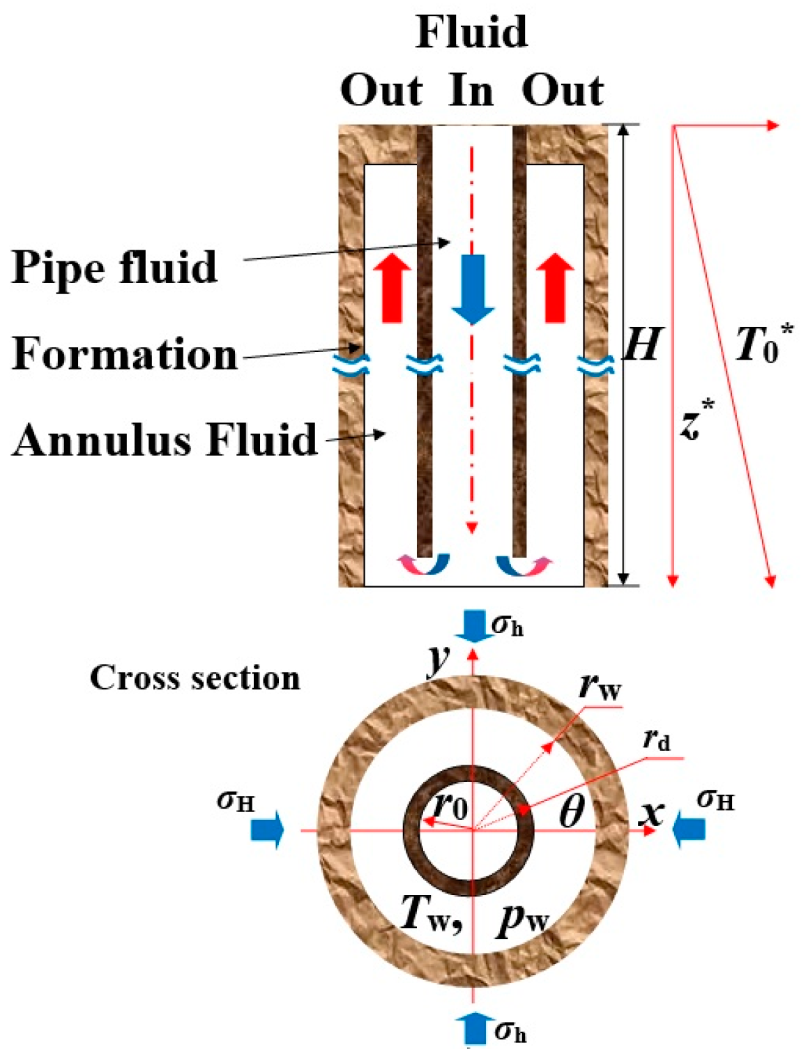
2.1. Problem Description

The geometry configuration for the present model of a W/R system is shown in Figure 1. The origin of the cylindrical coordinate system is set to coincide with the centre of the well at the surface. The system is initially in an equilibrium state with the formation temperature distribution T0* = A0 z + B0 [21], where A0 is the geothermal gradient and B0 is the surface soil temperature. At an arbitrary depth of z, the cross-sectional wellbore is subjected to maximum horizontal principal stress σH(z), minimum horizontal principal stress σh(z), vertical principal stress σv(z) and wellbore pressure pw(z). The temperatures of the fluid inside the annulus and tubing are denoted as Ta* and Td*, respectively, independent of the radius. The rock temperature is denoted as Tr*. The temperature on the borehole wall is denoted as Tw*. At time t > 0, a fluid with a given temperature Tin* is injected into the tubing at a mass rate Qd and returns to the surface along the annulus when it reaches the bottom of the tubing string. The return mass flow rate is denoted as Qa.
The wellbore radius is denoted by rw and the wellbore depth is H. The inner and outer radii of the tubing are r0 and rd, respectively. Therefore, the tubing wall thickness is denoted as δ0 = rd r0 and the effective width of the annulus is wa = rw rd.
For simplicity, the following assumptions are made: (1) the fluid is incompressible and the rock formation is impermeable, homogeneous, isotropic, linear and elastic; (2) the material properties are constants, independent of temperature change; and (3) the heat conduction along the vertical direction in the formation is neglected.

2.2. Governing Equations

2.2.1. Wellbore Heat Transfer

The fluid temperature in the tubing is determined by the heat exchange between the tubing and the annulus and the heat advection down the tubing. The fluid temperature in the annulus is determined by the heat exchange between the annular fluid and the surrounding rock, the heat exchange between the tubing and the annulus and the heat advection up along the annulus. According to Raymond [15], the advective heat transfer equations for fluids inside the tubing string and in the annulus are expressed as follows.
ρ l c l A d v d T d * z + 2 π r d h a d ( T d * T a * ) = ρ l A d c l T d * t , ρ l c l A a v a T a * z + 2 π r d h a d ( T d * T a * ) + 2 π r w h w ( T w * T a * ) = ρ l A a c l T a * t ,
where cl is the fluid specific heat capacity; Am and Tm* (m = d refers to tubing and m = a refers to annulus) denote the cross sectional area and the fluid temperature, respectively; had is the overall heat transfer coefficient (HTC) characterizing heat exchange between the fluids in the tubing and in the annulus through the tubing wall; and hw is the film HTC between the fluid in the annulus and the surrounding rock formation. The velocities vm (m = d or a) in the tubing and the annuls are expressed as
v a = Q a A a ρ l ,   v d = Q d A d ρ l ,   A a = π ( r w 2 r d 2 ) ,   A d = π r 0 2 .

2.2.2. Heat Conduction in Rock

As for the heat transfer in the rock formation, two simplifications can be made. First, as the temperature gradient in the radial direction is much greater than that in the vertical direction, the derivative of the formation temperature with respect to z can be ignored [15]. Then, the governing equation to describe the heat flow in the formation is written as
k r 2 T r * = ρ r c r T r * t + γ T R ε v t
where εv is the volumetric strain. Second, according to the analysis by Coussy [44] and Wu et al. [39], the deformation induced temperature change is very small so that it can be ignored. Therefore, the second term on the right side of Equation (2) is omitted in the present work.

2.2.3. Rock Deformation

The following governing equations in a polar coordinate system (r, θ) are used to describe the mechanical responses of the rock formation, whose temperature distribution is disturbed by the circulating fluid.
  • Equations of equilibrium
    σ r r r + 1 r σ r θ θ + σ r r σ θ θ r = 0 ,   σ r θ r + 1 r σ θ θ θ + 2 σ r θ r = 0
  • Strain-displacement relations
    ε r r = u r r ,   ε θ θ = u r r + 1 r u θ θ ,   ε r θ = 1 2 [ 1 r u r θ + u θ r u θ r ]
  • Linear TM constitutive equation for isotropic medium
    σ i j = 2 G [ v 1 2 v δ i j ε v + ε i j ] δ i j γ T r
In the above equations, σij is the stress change tensor (positive is tension) and is equal to σij*σijR, the difference between the total stress σij* and the initial stress σijR; εv is the volumetric strain and εij the strain tensor; Tr = Tr*T0* denotes the rock temperature change; G, v and K = 2G(1 + v)/3(1 − 2v) are shear modulus, Poisson’s ratio and bulk modulus for the rock formation, respectively; α is the coefficient of volumetric thermal expansion of the rock formation; γ = αK; and δij is Kronecker’s delta.

2.3. Boundary Conditions

The fluid temperature at the inlet of the tubing is specified during drilling. In order to satisfy the continuity condition, the temperature of fluids in the tubing and in the annulus at the bottomhole should be identical. Thus, we have
T d * ( z ,   t ) = T in * , at   z = 0 , T d * ( z ,   t ) = T a * ( z ,   t ) , at   z = H .
In addition, at the wellbore wall, the heat flux from the formation is equal to the heat flux into the wellbore, i.e., the following continuity condition must be met
2 π r w h w ( T r * T a * ) = 2 π r w k r T r * r ,   at   r = r w .
The pressure at the wellbore wall at a depth z is assumed to be time-independent and is approximated by
p w ( z ) = ρ l g z ,
where g is the gravitational acceleration.
The initial condition of the system is given as
T d ( z , t ) = T a ( z , t ) = T r ( z , r , t ) = 0 ,   on   t = 0 .
where Tm = Tm*TR (m = d refers to tubing, m = a refers to annulus and m = r refers to formation).
The remote boundary conditions are expressed in terms of changes of temperature and stresses
T r = 0 on   r , σ r r = 0 , on   r , σ r θ = 0 , on   r ,
while at the wellbore wall, the stress boundary conditions are
σ r r = p w ( p 0 + s 0 cos 2 θ ) on   r = r w , σ r θ = S 0 sin 2 θ on   r = r w ,
where
p 0 = σ H max + σ H min 2 ,   s 0 = σ H max σ H min 2 .

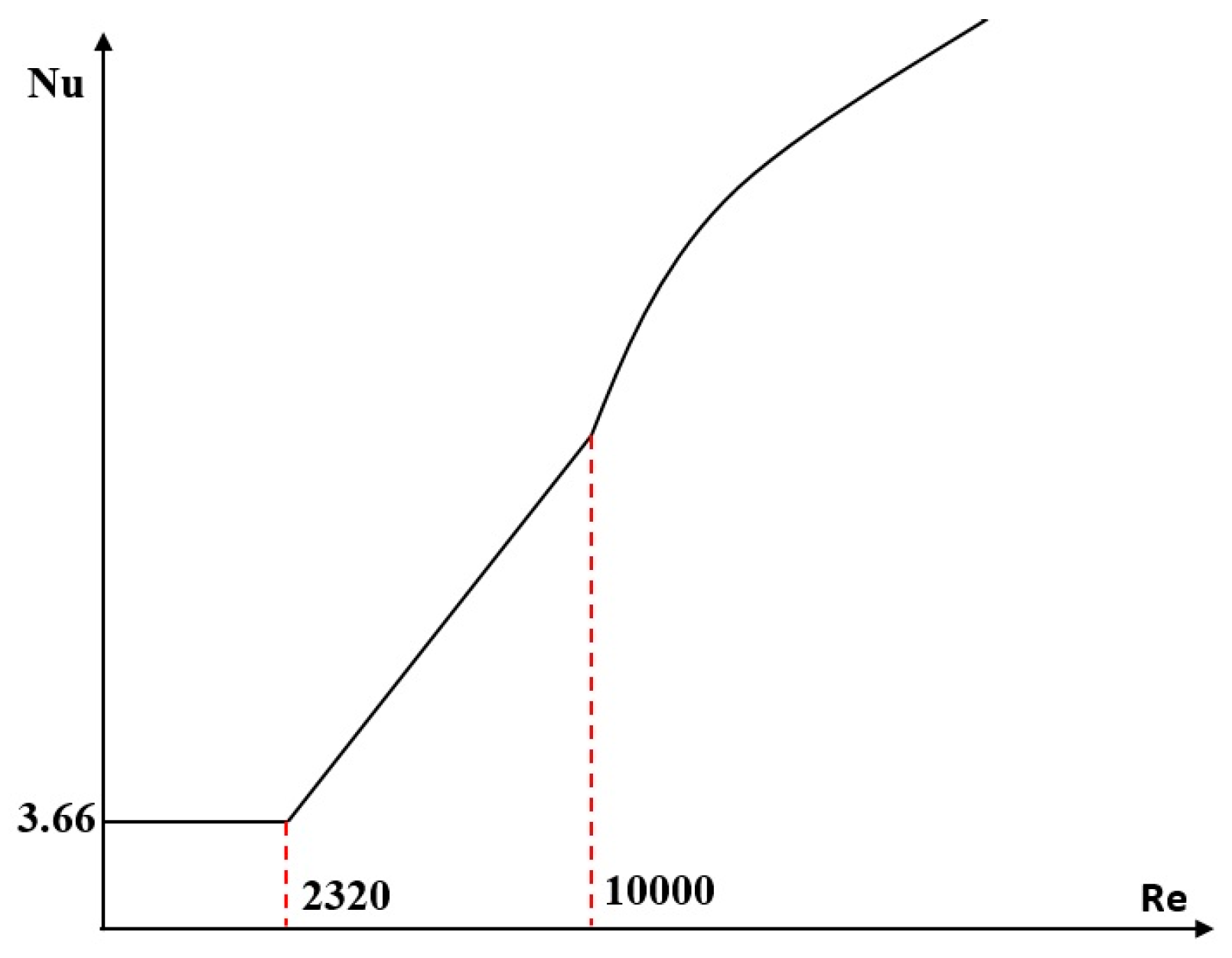
2.4. Heat Transfer Coefficients (HTCs)

In the present paper, the value of the HTC for forced advection along a pipe is calculated by
HTC = N u k l D ,
where kl is the fluid thermal conductivity, D is the hydraulic diameter (a characteristic length) and Nu is the dimensionless Nusselt number. If the Nusselt number is known, the HTC value can be obtained.
When Re ≤ 2320, the flow is laminar and Nu is equal to be 3.66. When Re ≥ 10,000, the flow is turbulent and the Nusselt number is calculated with the Mikheev equation [45] which is reported to be the reliable formula for estimating the HTC for the flow of Newtonian fluids in a tube. In particular, the Nusselt numbers for turbulent flow at the inner tubing and wellbore walls, respectively, are given by Isachenko and Osipova [46] as follows
N d = h d ( 2 r 0 ) k l = 0.021 ( Re d ) 0.8 ( Pr l ) 0.43 ( Pr l / Pr d ) 0.25 , N a = h a ( 2 w a ) k l = 0.021 ( Re a ) 0.8 ( Pr l ) 0.43 ( Pr l / Pr r ) 0.25 ,
where μ is the fluid dynamic viscosity, and kj, ρj and cj are the thermal conductivity, mass density and specific heat capacity (here the symbol j = l, d or r denotes the liquid, tubing or rock), respectively. The Reynolds number for fluid flow in the tubing and annulus and the Prandtl number are defined below
Re d = ρ l v d 2 r 0 μ ,   Re a = ρ l v a 2 w a μ ,   Pr d = μ c d k d ,   Pr l = μ c l k l ,   Pr r = μ c r k r .
When 2320 < Re < 10,000 (for transition flow), a linear interpolation method is used, as show in Figure 2.
The overall HTC across the tubing wall is determined by the empirical formula derived by Willhite [47], which gives
1 h a d = 1 h d + 1 k d / δ 0 + 1 h a ,

3. Dimensional Analysis

By using the following transformation
Θ a = T a * T R A 0 H ,   Θ d = T d * T R A 0 H ,   Θ r = T r * T R A 0 H ,   Θ in = T in * B 0 A 0 H , Σ i j = σ i j G ,   Ω i = u i r w ,   R = r r w ,   τ = d r t r w 2 ,   Z = z H ,   B i = h a r w k r , d r = k r ρ r c r ,   β = 2 ( 1 v ) 1 2 v ,   c = γ A 0 H G ,   a 1 = γ ρ r c r ,   a 2 = B 0 A 0 H
the governing Equation (1) for heat transfer in the wellbore and heat exchange with reservoir is rewritten as
χ d Θ d τ + Θ d z = b [ Θ a Θ d ]   1 , χ a Θ a τ Θ a z = d [ Θ a Θ d ] e [ Θ a Θ w ] + 1 ,
where the coefficients are defined as
χ d = H d r r w 2 v d ,   χ a = H d r r w 2 v a ,   b = 2 N a d ζ H P e d ζ 0 ,   d = 2 N a d ζ H P e a ( 1 + ζ d ) ,   e = 2 N w ζ H P e a ( 1 ζ d 2 ) , N a d = h a d 2 r d k l ,   ζ H = H r w ,   ζ 0 = r 0 r w ,   ζ d = r d r w ,   Φ = Q a Q d ,   ε d = k d k l ,   ε r = k r k l .
The stress–strain correlation (5) is given as
Σ i j = ( β 2 2 ) δ i j Ξ v + 2 Ξ i j δ i j c Θ r
and the strain-displacement relationship is rewritten as
Ξ r r = Ω R R ,   Ξ θ θ = Ω R R + 1 R Ω θ θ ,   Ξ r θ = 1 2 [ 1 R Ω R θ + Ω θ R Ω θ R ] .
In addition, heat conduction in the rock formation becomes
2 Θ r = Θ r τ
The boundary and initial conditions for the wellbore become
Θ r R = B i [ Θ r Θ a ] , on   R = 1 , Θ d = Θ in , on   Z = 0 , Θ d = Θ a   , on   Z = 1 , Θ r = Θ d = Θ a = 0 , on   τ = 0 .
and the boundary conditions for the reservoir are rewritten as
Θ r = 0 on   R , Σ R R = 0 , on   R , Σ R θ = 0 , on   R ,
While, at the wellbore wall, the stress boundary conditions are
Σ R R = Π w ( P 0 + S 0 cos 2 θ ) on   r = r w , Σ R θ = S 0 sin 2 θ on   r = r w ,  
where
Π w = p w G ,   P 0 = p 0 G ,   S 0 = s 0 G .

4. Solution Method

From Equations (1)–(11) we find that the heat transfer and deformation process represent a linear system. By using the same approach as that in [27,39], the non-hydrostatic remote stresses are decomposed into isotropic and deviatoric components, i.e., p0 and s0. According to the superposition principle, the present problem can be solved by studying two loading modes, i.e., isotropic (Mode 1) and anti-symmetric (Mode 2). In Mode 1, the fluid circulates in the wellbore that is subjected to the isotropic far-field stress p0, wellbore pressure and initial temperature conditions, while in Mode 2 the wellbore is subjected to the anti-symmetric far-field stress s0 and homogenous boundary conditions. The final solutions of near-well stress fields are the combination of the above results. It should be mentioned that the wellbore temperature varies with circulation time. In addition, the temperature evolution in the pipe and annulus can be obtained analytically in Laplace space.
The Laplace transformation is defined as
F ^ ( s ) = + e s τ f ( τ ) d τ
where s is a complex number and the symbol ^ denotes the Laplace transform of a quantity ( Θ ^ a , Θ ^ d , Θ ^ r , Σ ^ R R , Σ ^ θ θ and Σ ^ R θ for example).
The stress boundary condition for the Mode 1 and Mode 2 problems are
Σ R R = Π w P 0   on   R = 1 , Σ R R = 0   on   R ,
and
Σ R R = S 0 cos 2 θ on   R = 1 , Σ R R = 0 on   R , Σ R θ = S 0 sin 2 θ on   R = 1 , Σ R θ = 0 on   R ,
respectively.
In Mode 1, it should be noted that Ω θ = 0 and Σ R θ = 0. Substitution of Equation (16) into the dimensionless forms of Equations (2) and (3) leads to the volumetric strain
δ v = c β 2 Θ r + C 0
where the constant C0 is equal to zero as δv vanishes at infinity. After putting δv into Equation (19), we obtain
2 Θ r = Θ r τ
By applying the Laplace transformation to the above equation, the following ordinary differential equation (ODE) is obtained for the rock temperature change
s Θ ^ r = 1 R d Θ ^ r d R + d 2 Θ ^ r d R 2
whose solution in Laplace space is obtained as
Θ ^ r = F 1 ( Z , s ) K 0 ( s R ) + F 2 ( Z , s ) I 0 ( s R ) .
where In and Kn denote the modified Bessel functions of the first and second kind of order n, respectively; and F1(s) and F2(s) are unknowns to be determined by the boundary conditions. Considering zero rock temperature change at infinity, the function F2(Z, s) = 0 and then
Θ ^ r = F 1 ( Z , s ) K 0 ( s R ) ,   Θ ^ w = F 1 ( Z , s ) K 0 ( s )
By using the first boundary condition in Equation (20), the annulus temperature change is found
Θ ^ a = Λ F 1 ( Z , s ) ,   where   Λ = K 1 ( s ) s / B i + K 0 ( s )
After applying the Laplace transformation to Equation (16), we obtain the following ODEs
f Θ ^ d + d Θ ^ d d Z = b Λ F 1 1 s , h F 1 Λ d F 1 d Z = d Θ ^ d + 1 s ,
whose solutions are found to be
F 1 ( Z , s ) = Q 1 ( s ) e λ 1 Z + Q 2 ( s ) e λ 2 Z + C 1 , Θ ^ d ( Z , s ) = C 2 Q 1 ( s ) e λ 1 Z + C 3 Q 2 ( s ) e λ 2 Z + C 4 ,
and then we have
Θ ^ a ( Z , s ) = [ Q 1 ( s ) e λ 1 Z + Q 2 ( s ) e λ 2 Z + C 1 ] Λ , Θ ^ r ( R , Z , s ) = [ Q 1 ( s ) e λ 1 Z + Q 2 ( s ) e λ 2 Z + C 1 ] K 0 ( s R ) ,
where the coefficients are defined as
C 1 = f d s ( f h d Λ b ) ,   C 2 = ( Λ λ 1 + h ) d ,   C 3 = ( Λ λ 2 + h ) d ,   C 4 = Λ b h s ( f h d Λ b ) , λ 1 = h + f Λ + ( f Λ + h ) 2 4 d b Λ 2 2 Λ ,   λ 2 = h + f Λ ( f Λ + h ) 2 4 d b Λ 2 2 Λ , f = ( χ d s + b ) ,   h = ( χ a s + d + e ) Λ e K 0 ( s ) .
Based on the boundary conditions, the coefficients Q1(s) and Q2(s) are calculated to be
Q 1 ( s ) = ( s C 4 Θ in ) ( Λ C 3 ) e λ 2 + s C 3 ( C 4 Λ C 1 ) s [ C 3 e λ 1 ( Λ C 2 ) C 2 e λ 2 ( Λ C 3 ) ] , Q 2 ( s ) = ( Θ in + C 4 ) ( C 2 + Λ ) e λ 1 + s C 2 ( C 4 Λ C 1 ) s [ C 3 e λ 1 ( Λ C 2 ) C 2 e λ 2 ( Λ C 3 ) ] .
From Equation (18), we obtain the induced stresses for Mode 1 if the radial displacement is known
Σ R R = 2 Ω R R ,   Σ θ θ = 2 c β 2 Θ r + 2 Ω R R ,   Σ z z = 2 c β 2 Θ r
Based on Equations (3), (25) and the second of Equation (31), we obtain the radial displacement
Ω R = Λ K 1 ( s R ) s + W ( s ) R
where W(s) is an unknown function and is calculated by the stress boundary condition Equation (22) at the wellbore wall
W ( s ) = 2 Λ s K 1 ( s ) ( Π w P 0   ) s 2 s s .
The solution to the Mode 2 loading provides the temperature, deformation and stress induced by the anti-symmetric far-field stress.
Again, substitution of Equation (16) into the dimensionless forms of Equations (2) and (3) leads to the following equations
δ v R 1 β 2 1 R ϖ θ = c β 2 Θ R , 1 R δ v θ + 1 β 2 ϖ R = c β 2 1 R Θ θ .
Here the rotation displacement ϖ is defined as
ϖ = Ω θ R + Ω θ R 1 R Ω R θ .
The Laplace transforms of the variables δ v , Ω R , Σ R R , Σ θ θ , Θ r , ϖ and Ω θ are defined in the same way in Equation (23) in terms of δ ¯ v , Ω ¯ R , Σ ¯ R R , Σ ¯ θ θ , Θ ¯ r , ϖ ¯ and Ω ¯ θ . Under Mode 2 loading, these Laplace transformed quantities are expressed as follows
( δ ¯ v , Ω ¯ R , Σ ¯ R R , Σ ¯ θ θ , Θ ¯ r ) = ( δ ^ v , Ω ^ R , Σ ^ R R , Σ ^ θ θ , Θ ^ r ) cos 2 θ , ( ϖ ¯ , Ω ¯ θ , Σ ¯ R θ ) = ( ϖ ^ , Ω ^ θ , Σ ^ R θ ) sin 2 θ ,
where δ v , Ω R , Σ R R , Σ θ θ , Θ r , ϖ and Ω θ are all functions of R and s only.
By Laplace transformation, Equation (34) are changed into the following two ODEs
d δ ^ v d R 2 β 2 ϖ ^ R = c β 2 d Θ ^ r d R , δ ^ v R 1 2 β 2 d ϖ ^ d R = c β 2 1 R Θ ^ r .
The solutions of above ODE are found to be
δ ^ v = c β 2 Θ r + F ( s ) R 2 ,   ϖ ^ = β 2 F ( s ) R 2 ,
where F(s) is an unknown function to be calculated and thus the induced stresses are obtained from Equation (18)
Σ ^ R R = β 2 F ( s ) R 2 2 Ξ ^ θ θ , Σ ^ θ θ = β 2 F ( s ) R 2 2 Ξ ^ R R , Σ ^ R θ = 2 Ξ ^ R θ , Σ ^ z z = v ( Σ ^ R R + Σ ^ θ θ ) .
For Mode 2, the Laplace transforms of the governing Equation (19) is simplified to be
d 2 Θ ^ r R 2 + 1 R d Θ ^ r R 4 Θ ^ r R 2 = s Θ ^ r + a s F ( s ) R 2 ,
whose solution, combined with the far-field boundary conditions, is found to be
Θ ^ r = K 2 ( s R ) G ( s ) a F ( s ) R 2 .
As Θ ^ r = 0 at R = 1, the function G(s) is
G ( s ) = a F ( s ) K 2 ( s R ) .
Therefore, the induced temperature and volumetric strain are
Θ ^ r = F ( s ) a [ K 2 ( s R ) K 2 ( s ) 1 R 2 ] ,   Ξ ^ v = F ( s ) m 1 K 2 ( s R ) K 2 ( s ) + m 3 F ( s ) R 2 ,
where
m 1 = c a β 2 + a c ,   m 3 = 1 m 1 .
In addition, Ξ ^ v and ϖ ^ can be expressed through the geometric relationships in Laplace space as follows
Ξ ^ v = Ω ^ R R + Ω ^ R R + 2 Ω ^ θ R , ϖ ^ = Ω ^ θ R + Ω ^ θ R + 2 Ω ^ R R .
By using Equations (38), (42) and (43), the displacements are obtained to be
Ω ^ R = m 1 F ( s ) s q K 2 ( η ) [ K 1 ( ξ ) + 2 ξ K 2 ( ξ ) ] + m 3 F ( s ) 2 R + Q ( s ) R 3 , Ω ^ θ = 2 m 1 F ( s ) s q K 2 ( η ) K 2 ( ξ ) ξ + m 4 F ( s ) 2 R + Q ( s ) R 3 ,
where m4 = −β2. Thus, from the constitutive Equation (18), the stresses are obtained
Σ ^ R R = 2 m 1 F ( s ) K 2 ( η ) [ 1 ξ K 1 ( ξ ) + 6 ξ 2 K 2 ( ξ ) ] + 2 ( β 2 m 3 ) F ( s ) R 2 6 Q ( s ) R 4 , Σ ^ θ θ = 2 m 1 F ( s ) K 2 ( η ) [ 1 ξ K 1 ( ξ ) + ( 1 + 6 ξ 2 ) K 2 ( ξ ) ] + 6 Q ( s ) R 4 , Σ ^ R θ = 4 m 1 F ( s ) K 2 ( η ) [ 1 ξ K 1 ( ξ ) + 3 ξ 2 K 2 ( ξ 1 ) ] + ( β 2 m 3 ) F ( s ) R 2 6 Q ( s ) R 4 ,
where the function F(s) and Q(s) are calculated via the stress boundary conditions at R = 1
F ( s ) = 4 S 0 η K 2 ( η ) s H 1 ( s ) ,   Q ( s ) = S 0 6 s H 2 ( s ) H 1 ( s ) ,
where
H 1 ( s ) = 4 K 1 ( η ) m 1 2 η K 2 ( η ) ( m 3 β 2 ) , H 2 ( s ) = 12 K 3 ( η ) m 1 6 η K 2 ( η ) ( m 3 β 2 ) .
As the temperature, displacements, and stresses induced by both modes are known, complete solutions are easily obtained by superposition.

5. Results and Discussions

In this section, the physical solutions to the temperature and stresses are obtained by applying the Stehfest method [48]. The parameters used in the following calculations are listed in Table 1 unless otherwise specified.

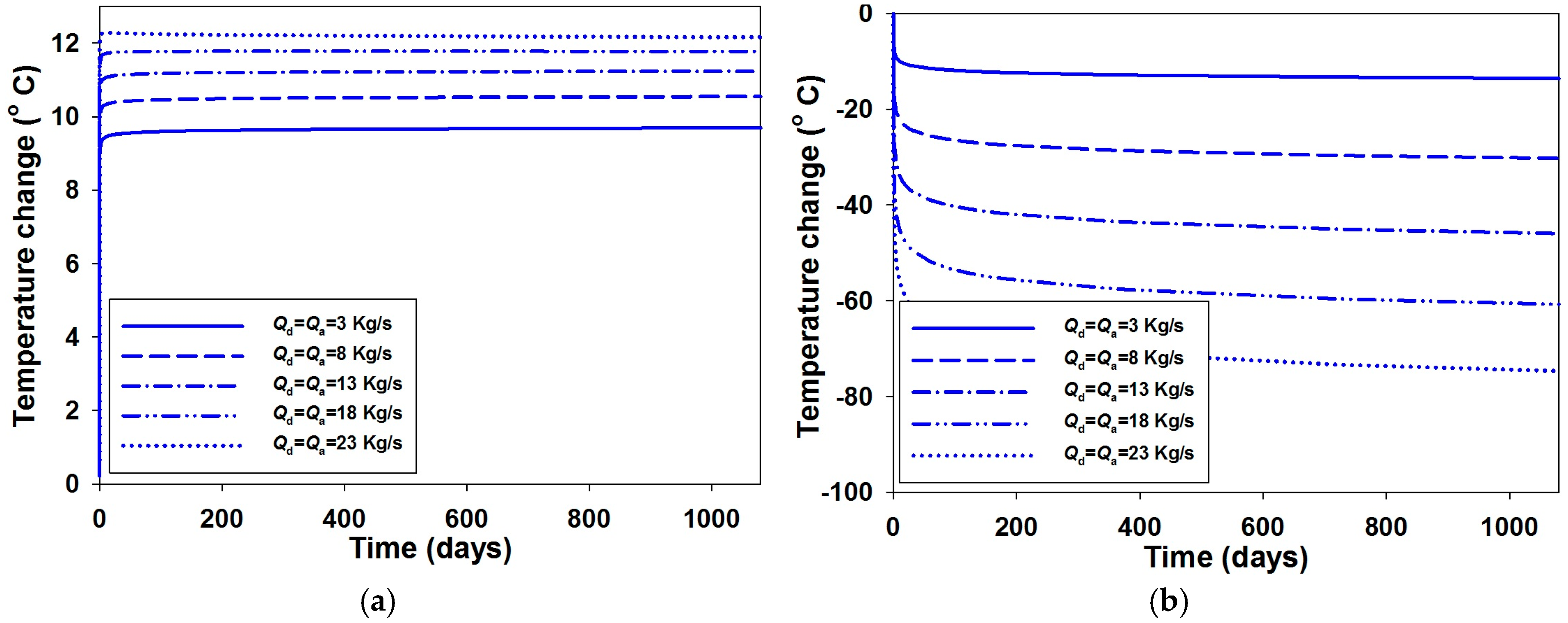
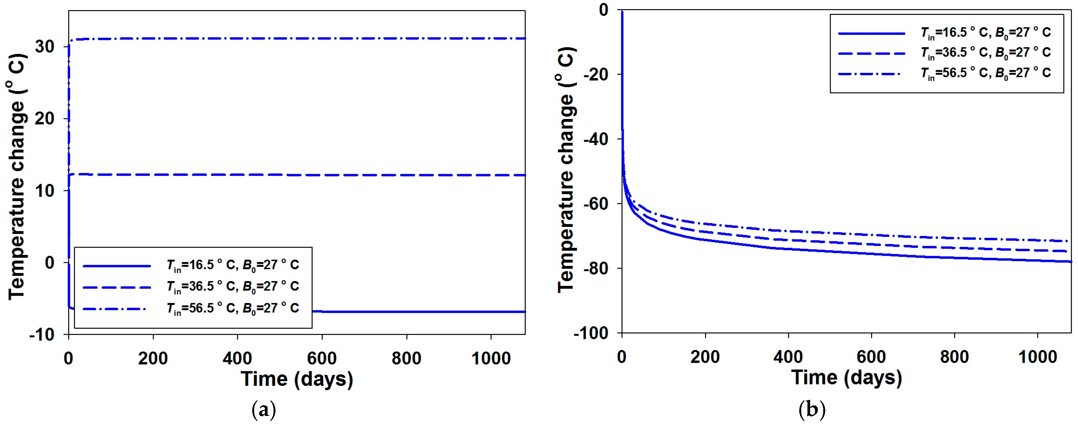
5.1. Wellbore Temperature Responses

The temperature responses in the wellbore/reservoir system can be calculated based on Equations (30) and (31).
Figure 3 shows the outlet and bottom-hole temperature changes for a range of injection rates. In Figure 3a, it can be seen that the outlet temperature change increases quickly (in about 2 h) to a certain value and then change very slowly after that time. In addition, when the injection rate increases from 3 Kg/s to 23 Kg/s, there is only a less than 3 °C difference between the outlet temperature changes. However, by increasing the injection rate, the bottom-hole temperature can be decreased quickly and by a significant amount as shown in Figure 3b. Therefore, changing the injection rate can be an efficient way to control the bottom-hole temperature and therefore the stress conditions near the wellbore, as shown by these simulations.
In Figure 4, the outlet and bottom-hole temperature changes for different injection temperatures are displayed. The injection rate is kept as a constant of 23 Kg/s. The bottom-hole temperature change decreases by 6 °C when the injection fluid temperature varies from 56.5 °C to 16.5 °C, even after a significant injection period, as shown in Figure 4b. This demonstrates that, to manage bottom-hole temperature and bottom-hole stress conditions, it is more effective to control the injection rate, rather than control injection fluid temperature for a deep wellbore.
In contrast, for a constant injection rate, the outlet fluid temperature is determined to a certain degree by the injection fluid temperature. In addition to the heat carried by fluid flowing up the annulus, the region near the outlet undergoes a quick heat exchange with the injection fluid. Therefore, if the injection temperature is lower than the surface soil/rock temperature, the outlet region is in a cooled. This can be seen in Figure 4a, where the outlet fluid temperature change varies from about −6 °C to 31 °C when the injection fluid temperature changes from 16.5 °C to 56.5 °C and the initial surface temperature B0 is fixed as 27 °C.
The fluid temperature profiles along the wellbore for two injection fluid temperatures (16.5 °C and 56.5 °C) are plotted in Figure 5. It should be mentioned that Z in the y axis denotes the dimensionless depth, i.e., Z = z/H. In both cases, the rock temperature in the lower portion of the wellbore decreases with time while that in the upper portion of the wellbore depends greatly on the injection fluid temperature. This makes the wellbore behave in a relatively complicated thermal manner and leads to the stress increasing or decreasing at different depths along the wellbore through heat exchange with the surrounding rock. Therefore, a transient analysis of coupled heat exchange for the W/R system is required.

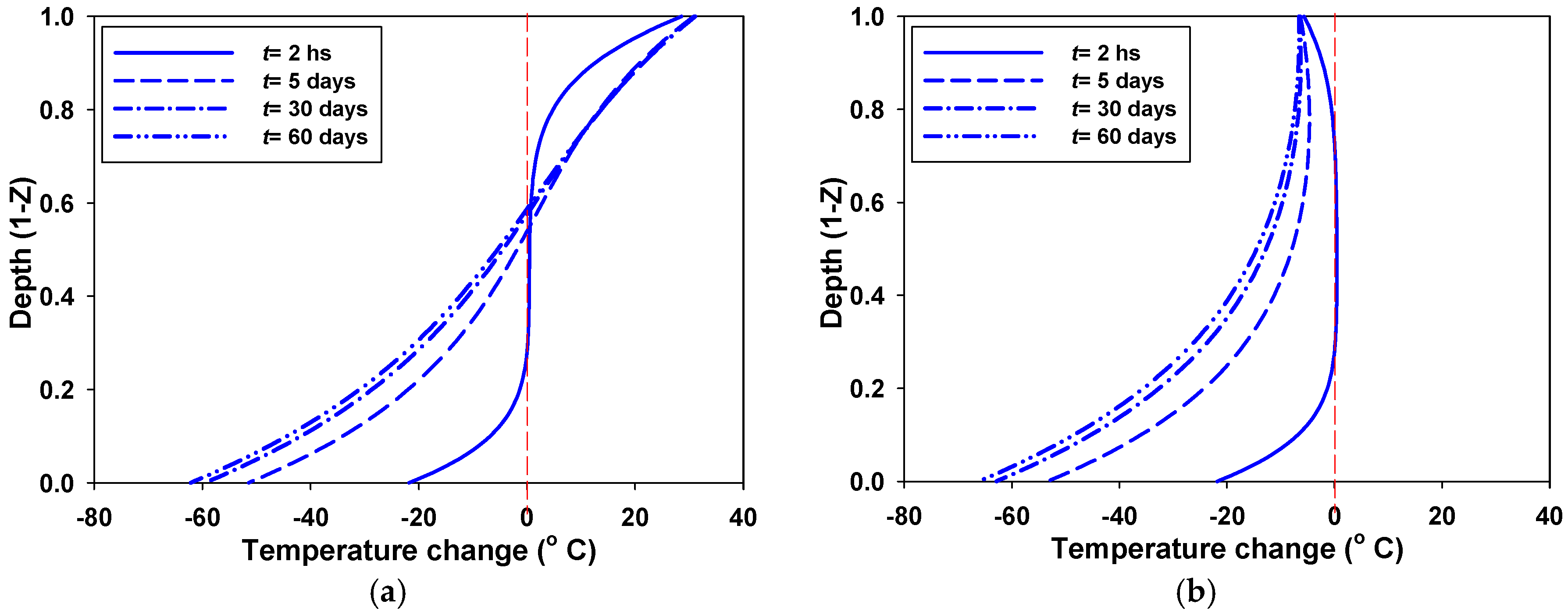
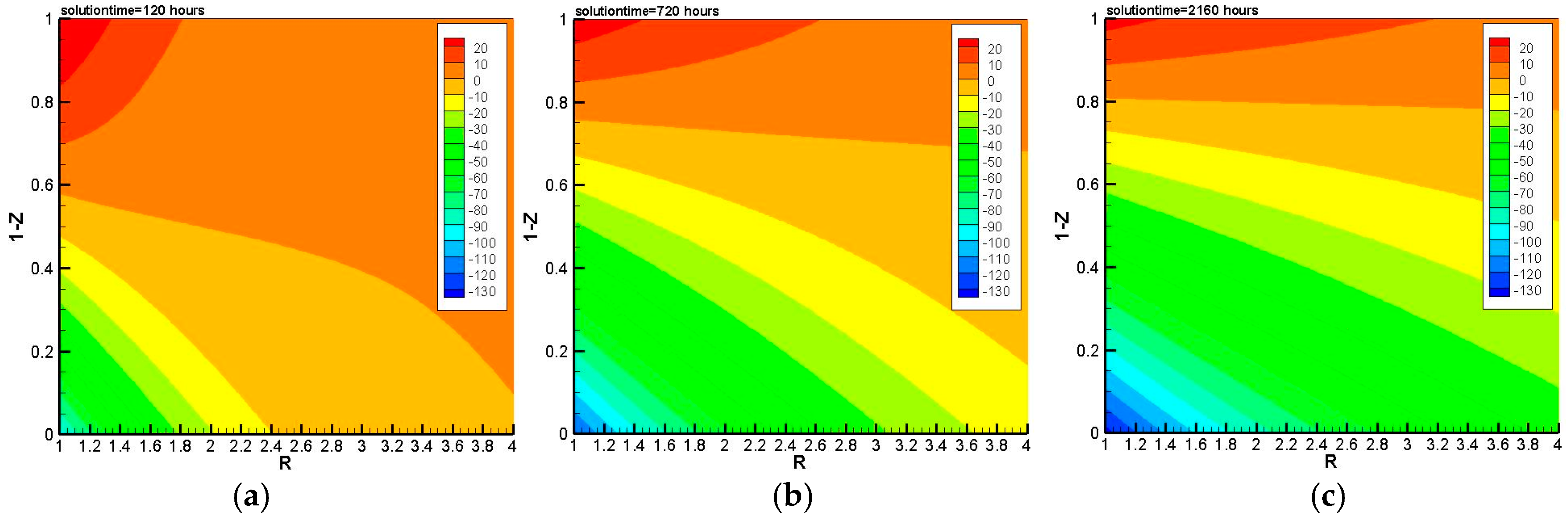
5.2. Temperature Change Near the Wellbore in the Rock

Figure 6 shows the contours for the temperature changes around the circular well at different times. Here Z and R denote the dimensionless depth and radial distance from the center of the wellbore, respectively, i.e., Z = z/H and R = r/rw. It can be seen that the near-well region at the bottom of the well is greatly impacted by the circulation. The low temperature area near the bottom of the well extends into the formation to a depth of one wellbore radius after 120 h. This cooled zone will induce thermo-elastic stresses that may be useful in helping initiate fractures and to enhance the permeability of certain natural fracture sets during stimulation.
It should be noted that, at the initial time of circulation, the upper part of the well is heated due to the hotter fluid flowing upwards, thus leading to enhanced compressive stress in the near-wellbore region. This may cause wellbore failure in terms of breakout. Therefore, some measure needs to be taken to prevent heat from loss into the formation by using casing with low thermal conductivity during the initial stage.

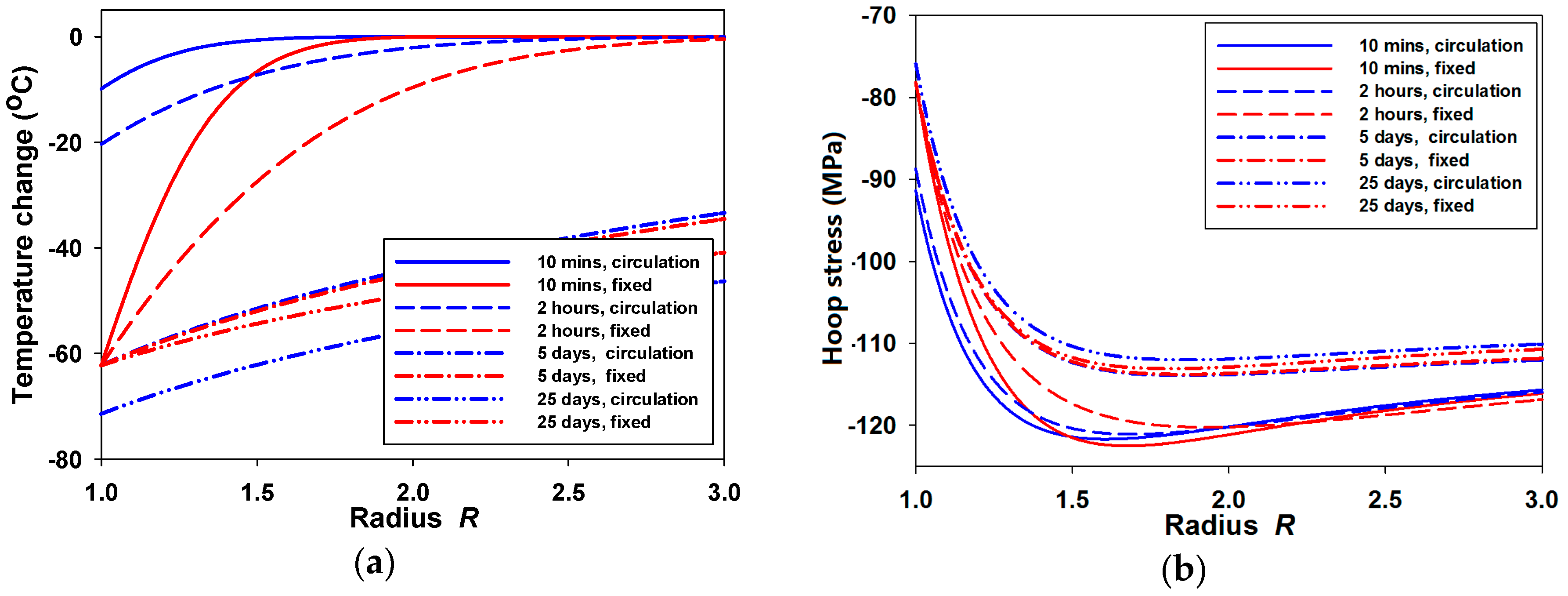
5.3. Comparisons of Near-Well Temperature and Stresses for a System Subject to Fixed and Variable Wellbore Temperature

In this section, a comparison of near-well temperature and stress change is made for two cases, i.e., one with constant wellbore temperature (Case 1, the wellbore wall experiences a step temperature change) and the other with varying temperature that is dependent on the fluid circulation history (Case 2).
Figure 7 shows the temperature and hoop stress variations in the σHmax direction at the wellbore bottom for Case 1 where the bottom-hole temperature is assumed to take a step change and be equal to the bottom-hole temperature after circulating for five days, and Case 2 where the circulation rate is equal to 28 Kg/s. Obviously, for Case 1, the rock temperature starts from the same point as the temperature on the wall that is fixed and increases with the distance away from the wellbore at a specific time. However, for Case 2, the rock temperature at the near-well region decreases with circulation time. There exists a region where the temperature predicted from the circulation case is higher than that from the fixed wellbore temperature case before the time t = 5 days. If we increase the circulation time (to say 25 days), the rock temperature will further decrease, thus leading to a region where the temperature predicted from the circulation case will be lower than that from the constant wellbore temperature case.
Due to different temperature responses predicted from the above two cases, the stress responses in the rock formation near the wellbore are also different. In Figure 7b, it can be seen that for a very small circulation time, the difference of the hoop stresses near the wellbore predicted from the two cases is significant. With time elapsed, the region with significant stress difference expands. At the time t = 5 days, the hoop stresses predicted from both cases are very close as the temperature changes in both cases have a similar profile. After five days, the difference of the hoop stresses for both cases becomes larger as the bottom-hole temperature in the circulation case continues to decrease with time.
Therefore, based on the circulation time, the conventional wellbore stability model with constant well temperature assumptions may over- or under-estimate the breakdown pressure (or mud weight) of the wellbore.

6. Conclusions

This paper presents a transient analysis of temperature and stress changes inside the wellbore and in the formation during fluid circulation. In particular, the solutions are derived for simultaneously solving fluid circulation along the wellbore and elastic deformation in the formation, through a unique temperature profile. By using the Laplace transformation and superposition method, the analytical solutions in the Laplace space are obtained. Numerical inversion is carried out to obtain the solutions in the time domain. The following conclusions are drawn based on the numerical results:
  • The fluid circulation rate plays a dominant role in the temperature evolution of the W/R system. The higher circulation rates (say cooling), the larger bottom-hole temperature change and thus the larger induced tensile stresses around the wellbore.
  • The effect of the injection fluid temperature on the outlet rock temperature change occurs rapidly. The outlet rock temperature change reaches a value quickly and is almost unchanged after that time.
  • The rock temperature of the upper part of the wellbore is determined mainly by the injection condition. It is possible for the upper open-hole section to develop breakouts due to the thermal stresses induced by the heating. Therefore, both wellbore cooling and heating should be taken into account during wellbore stability analysis.
  • This work provides a more consistent prediction on the temperature evolution and stress distribution along the wellbore resulting from the variable well temperature profiles associated with fluid circulation, thus making possible a more accurate wellbore stability analysis. The analysis for fixed boundary condition may over- or under-estimate the stress conditions around the wellbore, thus leading to inaccurate prediction of the mud weight density required to maintain a stable well.
  • Based on the first two points, varying circulation rates may be a more efficient way to manage bottom-hole temperature and bottom-hole stress conditions, rather than changing injection fluid temperature.

Acknowledgments

The authors thank CSIRO for permission to publish the research outcomes. This work is supported by the National Natural Science Foundation of China (41502346) and Strategic International Cooperation Project in Science and Technology Innovation of National Key Research and Development (2016YFE0204300).

Author Contributions

Bisheng Wu developed the model and wrote the whole paper; Tianle Liu, Xi Zhang and Bailin Wu contributed to the analysis; Robert G. Jeffrey contributed to the abstract, introduction and conclusion sections. He contributed to proof reading the paper to improve the overall presentation; Andrew P. Bunger contributed to the analysis.

Conflicts of Interest

The authors declare no conflict of interest. The founding sponsors had no role in the design of the study; in the collection, analyses, or interpretation of data; in the writing of the manuscript, and in the decision to publish the results.

Nomenclature

(Note: The variables with symbol “^” denote the Laplace transform of the corresponding variables.)
A0Geothermal gradient (°C/m)Td*Fluid temperature in the pipe (°C)
AaAnnulus cross sectional area (m2)Tin*Injection fluid temperature (°C)
AdTubing cross sectional area (m2)Tr*Formation temperature (°C)
aiCoefficients defined by Equation (15) (i = 1 or 2)TrFormation temperature change (°C)
B0Surface soil temperature (°C)Tw*Wellbore wall temperature (°C)
BiBiot number defined by Equation (15)T0*Initial formation temperature (°C)
bCoefficient defined by Equation (17)urRadial displacement (m)
clFluid specific heat (J/(kg∙K))uθHoop displacement (m)
crRock specific heat (J/(kg∙K))vPoisson’s ratio
cdPipe specific heat (J/(kg∙K))vaFluid velocity in the annulus (m/s)
cCoefficient defined by Equation (15) vdFluid velocity in the tubing (m/s)
CiCoefficients in Equations (25) and (30) (i = 1 or 2)waAnnulus width wa = rwrd (m)
DHydraulic diameterz*Coordinate in the z direction (m)
dCoefficient defined by Equation (17)ZDimensionless coordinate in the z direction
drThermal diffusivity for the rock (m2/s)
eCoefficient defined by Equation (17)Greek symbols
f, hExpressions defined by Equation (29)αVolumetric thermal expansion coefficient (1/K)
gGravitational acceleration (m/s2)βElastic constant defined by Equation (15)
GShear modulus (Pa)γ=αK (Pa/K)
hadOverall heat transfer coefficient (W/m2K)λiExpressions defined by Equation (31) (i = 1 or 2)
haHTC between the fluid and formation (W/m2K)δ0Pipe thickness δ0 = rdr0 (m)
hdHTC between the fluid and inner tubing (W/m2K)δijKronecker’s delta
HWellbore depth (m)ρlFluid mass density ρl (Kg/m3)
HiExpressions defined by Equation (46)ρdRock mass density ρr (Kg/m3)
klFluid thermal conductivity (W/(m∙K))ρrPipe mass density ρd (Kg/m3)
krRock thermal conductivity (W/(m∙K))μFluid viscosity μ (Pa∙s)
kdPipe thermal conductivity (W/(m∙K))ωDimensionless rotation displacement
KBulk modulus (Pa)σHMaximum horizontal principal stress (Pa)
miConstants in Equations (42) and (44) (i = 1, 2 or 4)σhMinimum horizontal principal stress (Pa)
NaNusselt number between fluid and formationσvVertical principal stress (Pa)
NadOverall Nusselt numberσijStress change tensor (Pa)
NdNusselt number between fluid and inner tubingσij*Total stress σij* (Pa)
NuNusselt numberσijRInitial stress (Pa)
PrdPrandtl numbers for the pipeΞijDimensionless strain tensor
PrlPrandtl numbers for the fluidΣijDimensionless stress change tensor
PrrPrandtl numbers for the formationПwDimensionless wellbore pressure
pwwellbore pressure (Pa)ΛExpressions defined by Equation (28)
p0Isotropic far-field stress (Pa)ΩiDimensionless displacement (i = R or θ)
P0Dimensionless isotropic far-field stressΘaDimensionless annulus fluid temperature change
QdInjection rate Qd (Kg/s)ΘdDimensionless pipe fluid temperature change
QaPump out rate Qa (Kg/s)ΘinDimensionless injection temperature change
QiExpressions defined by Equation (31) (i = 1 or 2)ΘrDimensionless formation temperature change
rCoordinate in the radial direction (m)τDimensionless time
RDimensionless coordinate in the radial directionχaCoefficient defined by Equation (17)
rdPipe outer radius (m)χdCoefficient defined by Equation (17)
r0Pipe inner radius (m)ζHRatio of wellbore depth to the wellbore radius
rwWellbore radius rw (m)ζ0Ratio of inner pipe radius to wellbore radius
ReaReynolds number for fluid flow in the annulusζdRatio of outer pipe radius to wellbore radius
RedReynolds number for fluid flow in the tubingεdRatio of thermal conductivity of pipe to fluid.
RDimensionless coordinate in the radial directionεrRatio of thermal conductivity of rock to fluid
sComplex number in Laplace transformationεijStrain tensor
s0Deviatoric far-field stress (Pa)εvVolumetric strain
S0Dimensionless deviatoric far-field stressΦRatio of production rate to injection rate
t*Time (s)
Ta*Fluid temperature in the annulus (°C)

References

  1. Khaksar, A.; Jalalifar, M.H.; Aslannejad, M. Analysis of vertical, horizontal and deviated wellbores stability by analytical and numerical methods. J. Pet. Explor. Prod. Technol. 2014, 4, 359–369. [Google Scholar]
  2. Caenn, D.R.; Darley, H.C.H.; Gray, G.R. Composition and Properties of Drilling and Completion Fluids, 7th ed.; Elsevier: Amsterdam, The Netherlands; Boston, MA, USA, 2017. [Google Scholar]
  3. Rahimi, R.; Asaba, M.; Nygaard, R. Analysis of analytical fracture models for wellbore strengthening applications: An experimental approach. J. Nat. Gas Sci. Eng. 2016, 36 Pt A, 865–874. [Google Scholar] [CrossRef]
  4. Lee, H.; Moon, T.; Haimson, B.C. Borehole breakouts induced in Arkosic sandstones and a discrete element analysis. Rock Mech. Rock Eng. 2016, 49, 1369–1388. [Google Scholar] [CrossRef]
  5. Sadeghalvaad, M.; Sabbaghi, S. The effect of the TiO2/polyacrylamide nanocomposite on water-based drilling fluid properties. Powder Technol. 2015, 272, 113–119. [Google Scholar] [CrossRef]
  6. Khaled, M.S.; Shokir, E.M. Effect of drillstring vibration cyclic loads on wellbore stability. In Proceedings of the SPE Middle East Oil & Gas Show and Conference, Manama, Bahrain, 6–9 March 2017. [Google Scholar]
  7. Kanfar, M.F.; Chen, Z.; Rahman, S.S. Effect of material anisotropy on time-dependent wellbore stability. Int. J. Rock Mech. Min. Sci. 2015, 78, 36–45. [Google Scholar] [CrossRef]
  8. Ma, T.; Wu, B.; Fu, J.; Zhang, Q.; Chen, P. Fracture pressure prediction for layered formations with anisotropic rock strengths. J. Nat. Gas Sci. Eng. 2017, 38, 485–503. [Google Scholar] [CrossRef]
  9. Llanos, E.M.; Zarrouk, S.; Hogarth, R.A. Numerical model of the Habanero geothermal reservoir, Australia. Geothermics 2015, 33, 308–319. [Google Scholar] [CrossRef]
  10. Bullard, E.C. The time necessary for a bore hole to attain temperature equilibrium. Geophys. J. Int. 1947, 5, 27–130. [Google Scholar] [CrossRef]
  11. Moss, J.T.; White, P.D. How to calculate temperature profiles in a water injection well. Oil Gas J. 1959, 57, 174–177. [Google Scholar]
  12. Edwardson, M.J.; Girner, H.M.; Parkison, H.R.; Williams, C.D.; Matthews, C.S. Calculation of formation temperature disturbances caused by mud circulation. J. Pet. Technol. 1962, 14, 415–426. [Google Scholar] [CrossRef]
  13. Tragesser, A.F.; Crawford, P.B.; Crawford, H.R. A method for calculating circulating temperature. J. Pet. Technol. 1967, 19, 1507–1512. [Google Scholar] [CrossRef]
  14. Ramey, H.J. Wellbore heat transmission. J. Pet. Technol. 1962, 14, 427–435. [Google Scholar] [CrossRef]
  15. Raymond, L.R. Temperature distribution in a circulating drilling fluid. J. Pet. Technol. 1969, 21, 333–342. [Google Scholar] [CrossRef]
  16. Holmes, C.S.; Swift, S.C. Calculation of circulating mud temperatures. J. Pet. Technol. 1970, 22, 670–674. [Google Scholar] [CrossRef]
  17. Keller, H.H.; Couch, E.J.; Berry, P.M. Temperature distribution in circulating mud columns. Old SPE J. 1973, 13, 23–30. [Google Scholar] [CrossRef]
  18. Sump, G.D.; Williams, B.B. Prediction of wellbore temperature during mud circulation and cementing operations. J. Eng. Ind. 1973, 95, 1083–1092. [Google Scholar] [CrossRef]
  19. Arnold, F.C. Temperature variation in a circulating wellbore fluid. ASME J. Energy Res. Technol. 1990, 112, 79–83. [Google Scholar] [CrossRef]
  20. Kabir, C.S.; Hasan, A.R.; Kouba, G.E. Determining circulating fluid temperature in drilling, workover, and well-control operations. SPE Drill. Complet. 1996, 11, 74–79. [Google Scholar] [CrossRef]
  21. Fomin, S.; Hashida, H.; Chugunov, V.; Kuznetsov, A.V. A borehole temperature during drilling in a fractured rock formation. Int. J. Heat Mass Transf. 2005, 48, 385–394. [Google Scholar] [CrossRef]
  22. Wu, B.; Zhang, X.; Jeffrey, R.G. A model for downhole fluid and rock temperature prediction during circulation. Geothermics 2014, 50, 202–212. [Google Scholar] [CrossRef]
  23. Kirsch, G. Die Theorie der Elastizität und die Bedürfnisse der Festigkeitslehre. Zeitschrift des Vereines deutscher Ingenieure 1898, 42, 797–807. [Google Scholar]
  24. Hiramatsu, Y.; Oka, Y. Stress around a shaft or level excavated in ground with a three-dimensional stress state. Mem. Fac. Eng. Kyotu Univ. 1962, 24, 56–76. [Google Scholar]
  25. Biot, M.A. General solutions of the equations of elasticity and consolidation for a porous material. J. Appl. Mech. 1956, 28, 91–96. [Google Scholar]
  26. Carter, J.P.; Booker, J.R. Elastic consolidation around a deep circular tunnel. Int. J. Solids Struct. 1982, 18, 1059–1074. [Google Scholar] [CrossRef]
  27. Detournay, E.; Cheng, A.H.D. Poroelastic response of a wellbore in a non-hydrostatic stress field. Int. J. Rock Mech. Min. Sci. Geomech. Abstr. 1988, 25, 171–182. [Google Scholar] [CrossRef]
  28. Rajapakse, R.D. Stress analysis of wellbore in poroelastic medium. J. Eng. Mech. 1993, 119, 1205–1227. [Google Scholar] [CrossRef]
  29. Ekbote, S.; Abousleiman, Y.; Cui, L.; Zaman, M. Analyses of inclined wellbores in poroelastic media. Int. J. Geomech. 2004, 4, 178–190. [Google Scholar] [CrossRef]
  30. Chen, G.; Yu, L. Consolidation around a tunnel in a general poroelastic medium under anisotropic initial stress conditions. Comput. Geotech. 2015, 66, 39–52. [Google Scholar] [CrossRef]
  31. Abousleiman, Y.; Cui, L. Poroelastic solutions in transversely isotropic media for wellbore and cylinder. Int. J. Solids Struct. 1998, 35, 4905–4929. [Google Scholar] [CrossRef]
  32. McTigue, D.F. Flow to a heated wellbore in porous, thermoelastic rock: Analysis. Water Resour. Res. 1990, 26, 1763–1774. [Google Scholar] [CrossRef]
  33. Kurashige, M. A thermoelastic theory of fluid-filled porous materials. Int. J. Solids Struct. 1989, 25, 1039–1052. [Google Scholar] [CrossRef]
  34. Charlez, P.A. Rock Mechanics. Volume 2. Petroleum Applications; Éditions Technip: Paris, France, 1997. [Google Scholar]
  35. Zhou, Y.; Rajapakse, R.K.; Graham, J. Coupled consolidation of a porous medium with a cylindrical or a spherical cavity. Int. J. Numer. Anal. Meth. Geomech. 1998, 22, 449–475. [Google Scholar] [CrossRef]
  36. Ghassemi, A.; Diek, A. Effects of thermal osmosis on shale instability. In Proceedings of the 4th North American Rock Mechanics Symposium, Seattle, WA, USA, 31 July–3 August 2000. Paper ARMA-2000-0231. [Google Scholar]
  37. Wang, Y.; Dusseault, M. A coupled conductive-convective thermo-poroelastic solution and implications for wellbore stability. J. Pet. Sci. 2003, 38, 187–198. [Google Scholar] [CrossRef]
  38. Choi, S.K.; Tan, C.P.; Freij-Ayoub, R. A coupled mechanical-thermal-physico-chemical model for the study of time-dependent wellbore stability in shales. Elsevier Geo-Eng. Book Ser. 2004, 2, 581–586. [Google Scholar]
  39. Wu, B.; Zhang, X.; Jeffrey, R.G.; Wu, B. A semi-analytic analysis of a wellbore in a non-isothermal low-permeable porous medium under non-hydrostatic stresses. Int. J. Solids Struct. 2012, 49, 1472–1484. [Google Scholar] [CrossRef]
  40. Wu, B.; Zhang, X.; Jeffrey, R.G. An extended overcore stress measurement method based on a thermo-poro-elastic analysis of the stresses in three-dimensional states. Int. J. Rock Mech. Min. Sci. 2016, 89, 75–93. [Google Scholar]
  41. Li, X.; Cui, L.; Roegiers, J.C. Thermo-poro-elastic analyses of inclined wellbores. In Proceedings of the SPE/ISRM Rock Mechanics in Petroleum Engineering, Trondheim, Norway, 8–10 July 1998; pp. 443–451. [Google Scholar]
  42. Abousleiman, Y.; Ekbote, S. Solutions for the inclined borehole in a porothermoelastic transversely isotropic medium. J. Appl. Mech. 2005, 72, 102–114. [Google Scholar] [CrossRef]
  43. Gao, J.; Deng, J.; Lan, K.; Song, Z.; Feng, Y.; Chang, L. A porothermoelastic solution for the inclined borehole in a transversely isotropic medium subjected to thermal osmosis and thermal filtration effects. Geothermics 2017, 67, 114–134. [Google Scholar] [CrossRef]
  44. Coussy, O. Poromechanics; John Wiley & Sons, Ltd.: Hoboken, NJ, USA, 2004. [Google Scholar]
  45. Mikheyev, M. Fundamentals of Heat Transfer; Peace Publishes: Moscow, Russia, 1960. [Google Scholar]
  46. Isachenko, V.P.; Osipova, V.A.; Sukomel, A.S. Heat Transfer; Energiya: Moscow, Russia, 1975. [Google Scholar]
  47. Whillhite, G.P. Over-all heat transfer coefficients in steam and hot water injection wells. J. Pet. Technol. 1967, 19, 607–617. [Google Scholar] [CrossRef]
  48. Stehfest, H. Algorithm 368: Numerical inversion of Laplace transforms. Commun. ACM 1970, 13, 47–49. [Google Scholar] [CrossRef]
Figure 1. Fluid circulation W/R system.
Energies 11 00042 g001
Figure 2. Calculation of the Nusselt number.
Energies 11 00042 g002
Figure 3. (a) Outlet; and (b) bottom-hole fluid temperature change under different injection rates.
Energies 11 00042 g003
Figure 4. (a) Outlet temperature change and (b) bottom-hole fluid temperature change for a range of injection fluid temperatures with Qd = Qa = 23 Kg/s.
Energies 11 00042 g004
Figure 5. Fluid temperature change along the wellbore for a range of injection temperatures: (a) Tin* = 56.5 °C; and (b) Tin* = 16.5 °C.
Energies 11 00042 g005
Figure 6. Contours for temperature change in the surrounding rock at different circulation times for Tin* = 36.5 °C, B0 = 27 °C and Qd = Qa = 25 kg/s; (a) t = 5 days, (b) t = 1 month; and (c) t = 3 months.
Energies 11 00042 g006
Figure 7. Comparison of the (a) temperature and (b) hoop stresses for the bottom-hole formation near the wellbore under variable and fixed boundary condition cases.
Energies 11 00042 g007
Table 1. Parameters for the calculations.
ParametersValue
Pipe internal radius r0 and thickness δ0 (m)0.0462, 0.01
Wellbore radius rw and height H (m)0.0762, 4131
Injection rate Qd and pump out rate Qa (Kg/s)23.0, 23.0
Injection and surface temperature Tin*, B0 (°C)36.5, 27
Formation geothermal gradient A0 (°C/m)0.047
Initial temperature T0* (°C)A0z + B0
Fluid and rock specific heat cl, cr (J/(kg∙K))4200, 790
Pipe specific heat cd (J/(kg∙K))460
Fluid, rock ther. conductivity kl, kr (W/(m∙K))0.68, 2.2
pipe thermal conductivity kd (W/(m∙K))50
Fluid and rock mass density ρl, ρr (Kg/m3)900, 2700
Pipe mass density ρd (Kg/m3)7800
Fluid viscosity μ (Pa∙s)0.0004
Thermal expansion coefficient α (1/K)5.0 × 10−6
Max horizontal, principal stress σH (MPa)−170
Min horizontal, principal stress σh (MPa)−130
Vertical, principal stress σv (MPa)−110
Shear modulus G (Pa)1.5 × 10¹⁰
Poisson ratio v0.25

