1. Introduction
The traditional grid is facing numerous challenges, including old infrastructure, lack of communication, increasing demand for energy, and security issues. To address these issues, the concept of smart grid has emerged which comprises of information and communication technologies that allow bidirectional communication between the utility and energy consumers. Broadly speaking, smart grid appears as a next generation grid and incorporates advanced technologies in communication, distributed generation, cyber security, and advanced metering infrastructure [
1]. These features of the smart grid ultimately enhance the efficiency, reliability, and flexibility of the power grid. The key objective of the smart grid is the transformation of the traditional grid to a cost effective and energy efficient power grid.
Demand side management (DSM) is an essential component in energy management of the smart grid. Generally, DSM refers to manage the consumer’s energy usage in such a way to yield desired changes in load profile and facilitates the consumers by providing them incentives [
2]. For this purpose, various DSM techniques have been proposed in literature, including peak clipping, valley filling, load shifting, strategic conservation, strategic load growth, and flexible load shape [
3]. Furthermore, DSM is capable of handling the communication infrastructure between end user and utility and also enables the integration of distributed energy resources to optimize energy consumption profile.
Recently, one of the crucial DSM activities is demand response (DR), it is presumed that DR is the subset of DSM in a broader aspect. DR is defined as the tariffs or programs established to influence the end users to reshape their energy consumption profile in response to electricity price [
4]. DR program is further categorized into two types: an incentive-based program and price-based program. An incentive-based program provides monetary incentive to the end user on the base of load curtailment. Various incentive programs are discussed in the literature, including direct load control (DLC), curtailable load, demand bidding and buy back, emergency and demand. On the other hand, a price-based program provides the price of electricity during different time intervals. The purpose of the price-based program is to reduce electricity usage when the electricity price is high and thus, reduce demand during peak periods. Price-based programs are: time of use (ToU), RTEP, inclined block rate, CPP, and day ahead pricing. DR is considered as a key feature in smart grid to improve the sustainability and reliability of power grid. However, it is examined in the literature that researchers considered the DSM and DR are interchangeable [
5,
6].
With the emergence of the smart grid, the consumer and the utility can exchange real-time information based on electricity pricing tariffs and energy demand of the consumer. The two way communication benefits not only the consumers, but also improve stability of the power grid. With this motivation, various models are designed to schedule energy consumption usage. Authors in [
7], comparatively evaluate the performance of home energy management controller (HEMC) which is designed to schedule energy consumption on the basis of heuristic algorithms: GA, binary particle swarm optimization (BPSO), and ant colony optimization (ACO). In [
8], authors aim to reduce electricity cost while incorporating renewable energy sources (RESs). The appliances are classified into five groups on bases of power ratings and time factor. Multiple knapsack problem (MKP) is used for the problem formulation and an optimization algorithm GA is employed to schedule the load profile. Jon et al. [
9], propose HEMS model for energy optimization and categorize the household appliances. The major objective of the proposed model is to tackle the uncertainties related to different kind of loads and reduce the electricity cost. The proposed algorithms are tested with the scrutiny of required home appliances and day-ahead pricing scheme.
Authors in [
10], present an improved model for the energy consumption of residential appliances. The desired objective is to minimize the cost by managing energy consumption of the appliances. Fractional programming (FP) is used for scheduling energy consumption by considering RTEP tariff and distributed energy resources. The work in [
11] presents HEMS model for energy optimization model at residential sector. The DSM techniques take into account in the presence of distributed generation, time-differentiated prices, and preference of loads. The minimization problem is solved using a constructive algorithm with GA while considering energy cost. Authors in [
12], provide a detailed study of HSA algorithm, the primary steps, its adaptation, and its specialty in different fields. Also, authors comparatively discuss the searching criteria of different optimization techniques and HSA. At the end, authors are elaborated the application of HSA in a complex scenarios and various fields. Authors in [
13], design day ahead scheduling model for microgrid systems with the integration RESs in order to minimize the start up cost and generation cost of the RESs. A hybrid algorithm is proposed using steps of enhance differential evolution (EDE) algorithm and HSA to achieve desired objective. The improvement in the tuning parameters of EDE and HSA are also carried out which enhances the search diversity. The work in [
14], demonstrates the residential load scheduling with the day ahead pricing scheme. A hybrid technique teacher learning genetic optimization (TLGO) is proposed to solve the optimization problem. The major objective of the work is to reduce electricity cost at minimum user discomfort.
Danish et al. in [
15], present HEMS model based on heuristic algorithm BSPO. The aim of the authors is to minimize the electricity cost while considering user comfort. Authors in [
16], present a generic model of DSM in order to optimize energy consumption in the residential sector. In a home environment, energy management controller (EMC) is used to control energy consumption of the appliances during peak hours. In [
17], authors propose a comprehensive model for energy management in homes with multiple appliances. The proposed model consists of six layered architecture and each layer is connected with other in order to achieve better results in terms of cost reduction and PAR.
The work in [
18] provides a comprehensive study of WDO technique, the basic concepts, structure its variants, and its application in electromagnetics. A numerical study is presented using uni-modal and multi-modal test functions and results of WDO and other optimization techniques, including GA, BPSO, and differential algorithm (DE). A recent work in [
19] proposes a novel approach of DSM with the integration of RESs. The energy provider inspects the load profile and the price of the electricity. Authors aim to reduce the deviation of average load energy demand by scheduling the energy consumption and storage devices. To solve scheduling problem, authors model the energy consumption and storage as a non-cooperative game.
In [
20], authors demonstrate the electricity load scheduling problem for multi-resident and multi-class appliances using problem ladson generalized bender algorithm while considering energy consumption constraint. The main objective of the study is to protect the private information i.e., energy consumption profile of the residences and maximize the users satisfaction.
Authors in [
21] give an insight of scheduling the energy management in the residential sector and propose two horizon algorithms. The proposed algorithms are efficient to reduce electricity cost with less computational time. Moreover, authors also discuss the implementation of proposed algorithms and challenges related to its implementation. Di Somma et al. in [
22], present stochastic programming model for the optimal scheduling of distributed energy resources system. The main aim of the study is to reduce energy cost and
emission while, satisfying time-varying user demand. In [
23], authors propose a model based on optimal economic choices for the management of the microgrid. The economic model is applied based on GA to the microgrid with traditional power plants and RESs. The work in [
24], provides an improved HEMS architecture considering various categories of appliances in the home. Multi- time scale optimization is formulated in order to schedule energy consumption of appliances. A predictive model-based-heuristic solution is proposed and its performance is compared with benchmark algorithms.
Table 1 lists the summary of the research work based on heuristic techniques.
HEMS is considered as an integral part for the successful DSM of the smart grid [
30]. HEMS provides an opportunity for the residential sector consumers to communicate with the household appliances and the utility to improve the energy efficiency regarding electricity tariff and consumer’s comfort. A wide range of research has been made to study scheduling problems in HEMS. A hybrid genetic particle swarm optimization (HGPO) is proposed to schedule the energy consumption of appliances in HEMS with the integration of RESs [
25]. However, it is impractical to schedule energy consumption without addressing user comfort. A heuristic optimization algorithm, such as GA is used to schedule appliances for the residential, commercial, and industrial sectors in [
26]. However, authors have not addressed the user comfort and also computational time of the algorithm is high. Similarly, in [
27,
28], integer linear programming (ILP) and dynamic programming (DP) are used to schedule the appliances and reduce electricity cost and PAR. However, these algorithms are inefficient in terms of computational time. In [
29], authors propose a general architecture of HEMS based on GA in the presence of RTEP and inclined block rate to reduce electricity cost and PAR. As GA is easy to implement, however, system deals with large number of appliances in multiple sector which increases the computational complexity.
Motivated from aforementioned literature work, we have proposed EHEMC, based on heuristic algorithms. The major contribution of this paper is summarized as follows:
We have proposed EHEMC with an objective to minimize electricity cost and average waiting time.
Initially, appliances are classified into three categories: regularly operated appliances, shiftable appliances, and elastic appliances-based upon their energy usage and time of operation. Furthermore, electricity cost and energy usage for each category are calculated using Equations (
2)–(
7).
To address our objective efficiently a hybrid optimization algorithm GHSA is proposed, which is later on compared with the existing algorithms, including WDO, HSA, and GA (
Section 3).
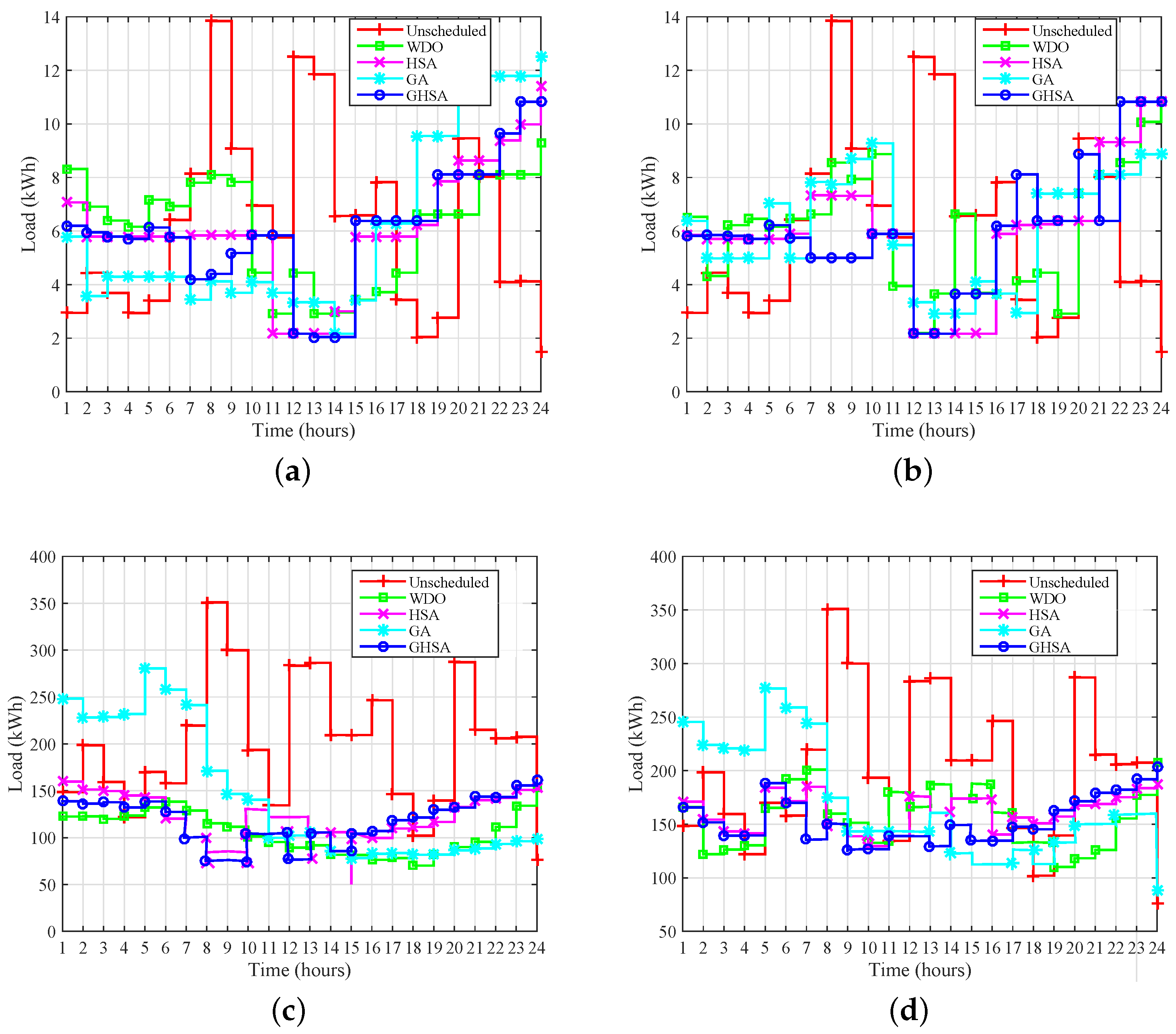
We implement the proposed GHSA algorithm for single home (SH) and multiple homes (MHs) and analyze its performance in the presence of pricing tariffs: RTEP and CPP. We observe that as the number of homes is increased computational time of the system also increases. However, our proposed algorithm GHSA effectively address the problem with less computation time.
In order to flexibly adjust the energy consumption profile different power ratings and operational time slots are assigned in MHs. Specifically, we consider fifty homes in MHs case.
The effect of electricity cost, energy consumption, and average waiting time is demonstrated by feasible regions (
Section 2.10).
The PAR is minimized to avoid peak power plants.
Finally, extensive simulations are conducted to validate the effectiveness of proposed algorithm GHSA in terms of electricity cost, PAR, and average waiting of the appliances.
The rest of the paper is structured as follows.
Section 2 presents a comprehensive study of the system model.
Section 3 describes the simulation results along with the discussion. At the end, we present the conclusion of the paper in
Section 4.
Nomenclature
This subsection presents the nomenclature as given in
Table 2. The table contains abbreviations, initialism, and pseudo-blends.
2. System Modeling
As mentioned before, for the effective deployment of smart grid, HEMS is crucial. HEMS can manage, control, and optimize energy consumption in home environment. While an essential element of HEMS, EHEMC is used to schedule energy consumption based on heuristic techniques to effectively reduce electricity cost while considering user preference.
The system model comprises of HEMS architecture, energy consumption model, load categorization, energy cost and unit price, and problem formulation.
2.1. HEMS Architecture
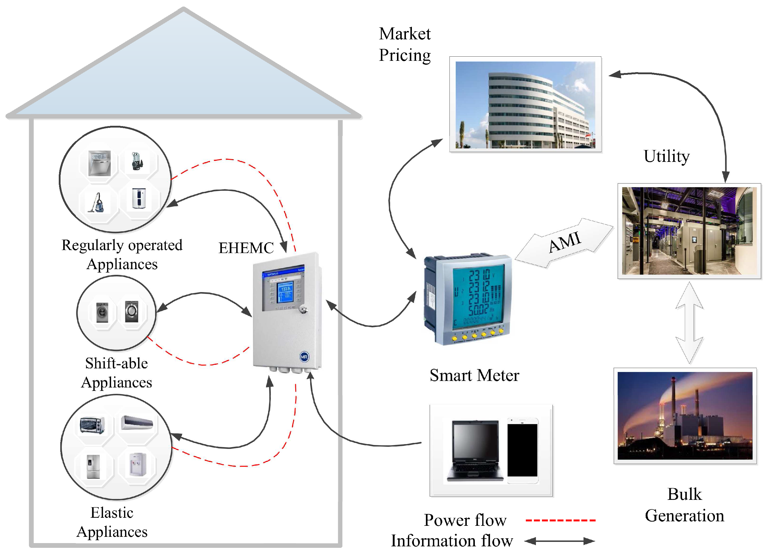
HEMS effectively visualizes the load consumption information in home and contributes towards the energy balancing between the supply and demand side. The primary aim of the HEMS implementation is to reduce electricity expense and PAR. According to utility perspective, its aim is twofold: first, it manages the energy consumption usage of residential sector consumers and secondly, it reduces PAR. While in consumers perspective, it reduces electricity expense. The proposed HEMS architecture comprised of advanced metering infrastructure (AMI), smart meter, EHEMC, In-home display, market pricing, utility, and bulk generation as shown in
Figure 1.
In general, AMI refers to measurement and collection of systems that include smart metering, advanced communications, and data management systems. AMI is also responsible to manage data collection and transmission of energy usage data from the smart meter to the utility. While smart meter acts as a communication gateway between the utility and smart home. The smart meter is associated with processing and sending of energy usage data from EHEMC to the utility via AMI and also processes electricity pricing signal from market pricing and utility. In HEMS architecture, it is assumed that each home is equipped with EHEMC. EHEMC consist of embedded system which schedules the energy consumption profile of the appliances in response to pricing signal and user comfort.
2.2. Energy Consumption Model
We consider a home with a set of appliances
, such that
represents each appliance over the time horizon
. Each time slot represents one hour and the total time interval is 24 h (
), in accordance with the single day. The total energy consumption of the appliances in a day can be mathematically represented as:
In smart grid, each home is equipped with EHEMC to optimize energy consumption and reduce electricity cost. Therefore, we categorize the appliances into three groups which are presented in the following subsection.
2.3. Load Categorization
We have categorized each appliance on the bases of energy consumption, operating time, and user preference. Suppose
represents a set of appliances, where
is regularly operated appliances,
shiftable appliances, and
elastic appliances.
Table 3 shows power ratings and time of operation of the appliances.
(1) Regularly operated appliances
These are also called fixed appliances because their energy consumption profile cannot be modified by EHEMC. They are vacuum pump, water pump, dishwasher, and oven. Regularly operated appliances are represented as
and their energy consumptions are represented by
. While power rating of
is expressed as
and the total energy consumption in a day is given as:
Similarly, the total cost per day of the
is given as:
where
is the operation state of appliances in time interval
and
represents the pricing signal.
(2) Shift-able appliances
These are controllable appliances and their operation time can be shifted to any time slot without performance degradation, however, once they turn ON their length of operation must be completed. They are also named as burst load for example, washing machine and cloth dryer. Shift-able appliances are denoted by
and power rating of
is
. The total energy is computed as:
The total cost calculated of
in a day is calculated as:
(3) Elastic appliances
These are considered as a flexible appliances i.e., their time period and energy consumption profile are flexibly adjusted. They are also named thermostatically-controlled appliances, such as water heater, air condition, water dispenser, and refrigerator. Let us consider
is the power rating of elastic appliances
and the total energy of
is computed as:
The total cost per day of
is given as:
Let us assume that the total energy consumed
by appliances in total time interval 24 h is given:
Similarly, total cost per day of
,
, and
appliances is calculated:
The energy consumption of each appliance in given time period can be mathematically shown in matrix form as:
2.4. Energy Cost and Unit Price
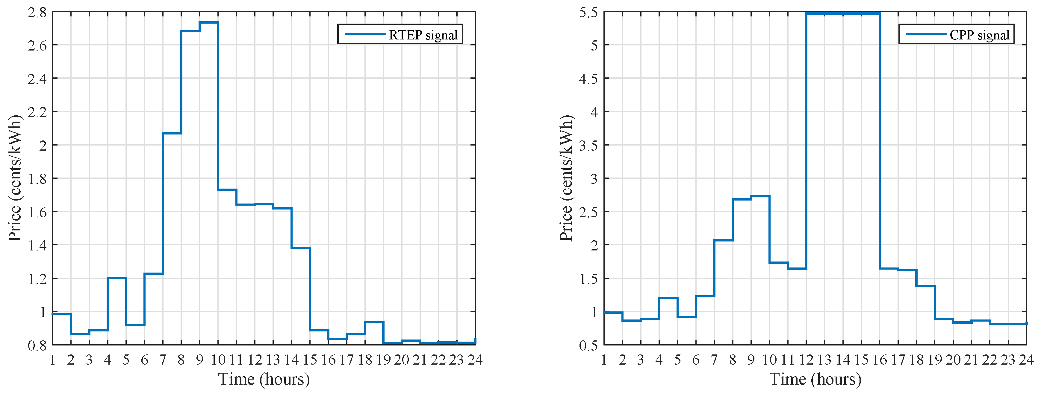
Various electricity tariffs are proposed to define electricity cost for a day or for a short time period. In our model, we consider RTEP and CPP tariffs.
The RTEP tariff is typically updated for each hour during a day and is capable of contributing better approximation of real time power generation cost. RTEP implementation requires two way of communication in order to interact with the consumer in a real time. Therefore, the aim of RTEP is to reduce demand of consumer during peak demand times. RTEP is also referred as dynamic pricing.
The CPP tariff has resemblance with ToU pricing regarding fix prices in different time intervals. The implementation of CPP during critical event imparts profitable response to the utility [
5]. However, due to stress on the power grid, the prices are replaced by the predefined higher rate in order to reduce energy demand. Thus, the aim of the CPP tariff is to assure the reliability and sustainability of the power grid.
In our research work, we consider RTEP and CPP tariffs because in normal operation of power grid, the RTEP behaves more flexibly as compared to other pricing signals. During critical conditions (high electricity demand and low generation) of the power grid consumers have to pay high electricity prices in the respective days or hours. Thus, both pricing signals are considered and electricity cost is reduced by scheduling energy consumption in off-peak hours.
2.5. Problem Formulation
In this research work, we considered SH and MHs with household appliances and our desired objectives are: to reduce electricity cost by scheduling energy consumption in low price hours (off-peak hours), to maintain grid stability by minimizing PAR, and to maximize user comfort level. We formulate our objective function using MKP approach which is based on the following assumptions:
Assuming as number of items .
Each of the items comprises of two attributes i.e., weight and the value. The weight of the items expresses the energy usage of the appliances in time interval . In addition, the value of the items denotes the energy cost of the appliances. However, the weight of the appliances is independent of the time interval.
We consider number of knapsacks in order to limit power consumption of each category of the appliances and also to limit the total power capacity .
By considering aforementioned assumptions, the utility and consumers can actively cooperate in energy demand management in order to reduce electricity cost and PAR. To achieve the grid sustainability, total energy consumption of the appliances in each time interval
should not exceed
. For this reason, we limit the total energy consumption as:
If the constraint in Equation (
11) is satisfied the inadequacy of power and stresses on the grid can be eliminated.
2.6. PAR
PAR is the ratio of the maximum aggregated load consumed in a certain time frame and the average of the aggregated load. PAR informs about the energy consumption behavior of the consumers and the operation of the power grid. The high PAR jeopardizes the grid stability and increases the electricity cost. While reduction in PAR simultaneously enhances the stability and reliability of the power grids and reduces the electricity bill of the consumers. Mathematically, it is expressed as:
and
show the maximum aggregated load and average load in a time frame (
t). While
represents the total energy consumption of the appliances in an hour.
2.7. User Comfort
In energy optimization, the load is shifted from peak hours to off-peak hours in order to reduce electricity cost. In this context,
consumption patterns are not changed and they must run with first preference, whereas
and
operation time interval (
) are flexibly shifted.
and
can be delayed to operate during peak hours to reduce electricity cost, however, it incurs discomfort to the consumer. To evaluate waiting time of appliances, we assume starting and ending time instant of appliances
and
, such that
and
is the request time of an appliance. While
is expressed as waiting time of the appliances.
Equation (
16) shows the average waiting time of the appliances and Equation (
17) represents the normalized value of average waiting time.
2.8. Objective Function
The objective is to minimize electricity cost and the average waiting time. The electricity cost is calculated using electricity pricing tariff and energy consumption. The total electricity cost per day is given by:
In Equation (
18)
shows the energy consumption of appliances in time slot
t and
indicates the electricity pricing tariff in time interval
t. Equation (
18) is normalized and is given as:
Now, we introduce objective function as:
subjected to:
In Equation (
20) both parts of the objective function i.e., minimization of total cost per day and average waiting time (
) of the appliances are first normalized using Equations (
17) and (
19) and then simultaneously solved using linear weighted sum method. Equal weights
and
are assigned to the both parts of the objective function i.e.,
=
= 0.5 [
29]. Equations (
21a)–(
21i) are constraints of the objective function. Equation (
21a) shows the total power consumption of appliances should not overreach the power grid capacity. Equation (
21b) limits the PAR less than
, and the ideal value of
is equal to 1. Equation (
21c) guarantees that time scheduled by appliances should not exceed the restriction. Equations (
21d) and (
21e) are constraints representing the energy load balance of
and
in any time slot
. While Equations (
21f) and (
21g) indicate the maximum and minimum energy consumption of
and
appliances in each hour of the operation. Equation (
21h) shows the maximum time that user postpone the operation of
and
. For our proposed model, we consider
of
and
is equal to or less than 5 h. Whereas, constraint (21i) clearly demonstrates the total energy consumption of the appliances in scheduled case and unscheduled case are always equal i.e., the EHEMC schedules the appliances by taking into account that appliances must complete their length of operation.
2.9. Optimization Techniques
Generally, mathematical techniques provide accurate solutions to the problem which is either feasible or infeasible. However, they are incapable of addressing the complex problems due to the curse of dimensionality, slow convergence rate, and complex calculations. While heuristic optimization algorithms do not guarantee the exact solution and provide approximate solutions, however, they are capable of handling complex calculations. In spite of approximate solutions, optimization algorithms are fair enough to converge faster, reach the desired solution, and applicable in all fields of engineering and computer science [
31]. For this purpose, we computed our problem as an optimization problem and four heuristic optimization techniques: WDO, HSA, GA, and GHSA are employed. Each heuristic optimization technique is explained as follows:
2.9.1. GA
GA is an adaptive algorithm based on the biological process [
26]. Initially, a set of random solutions is generated called chromosomes and the set of the chromosome is considered as a population. Each chromosome comprises of genes and the value of gene is either binary or numerical value. We consider the value of gene as 1 or 0 which actually shows ON and OFF states of the appliances. The fitness of each chromosome is evaluated using Equation (
20) and the stochastic operators crossover and mutation are used to generate new populations. Two point crossover with crossover rate
= 0.9 is used and the obtained chromosome is further mutated through mutation process which diversifies the search space of the algorithm, the mutation rate is considered
= 0.1. The process of crossover and mutation enables to reach at global optimal results. At the end, binary array [0 0 1 0 0 0 0 0 1 1] is obtained which shows the appliance is ON at 3, 9 and 10 location of the array. We then find out electricity cost and energy consumption to achieve our desired objective. The optimal results are obtained by considering the parameters in
Table 4.
The process is continued until the best optimal vector is achieved. Additionally, in comparison to other existing optimization techniques, GA is more robust and solves the complex non-linear problem with high convergence rate. GA also exhibits the property of independence of problem domain and imparts divergent solution in a single iteration.
2.9.2. WDO
WDO is the meta-heuristic algorithm which is inspired by the atmospheric motion of wind. In WDO, infinitely small air parcels move in a search space and wind blows to equalize pressure on air parcels using four different forces. These forces are cariols forces, pressure gradient forces, gravitational forces, and the frictional forces. Coriolis force tends to move the wind horizontally i.e., rotate the wind around the earth, while pressure gradient force is defined as; a change in wind pressure over distance covered by the wind. When both coriolis force and pressure gradient force are equal they balance the wind pressure horizontally. Furthermore, the gravitational force pulls the wind towards its center and it is in the vertical direction, while the friction force lowers the speed of the wind which in turn slow down the speed of coriolis force. All of these forces are expressed mathematically as [
15]:
At first, the random solution
is generated using Equation (
26).
Each of the random solution is evaluated using fitness function and relatively good solutions are reproduced, while bad solutions are neglected. In each step, position and the velocity of the air parcel is evaluated and the new value of velocity is assigned to each air parcel. Equation (
27) shows the updated velocity
of air parcels
After updating the velocity of the particle. New generation is obtained using Equation (
30) and the process will continue until stopping criteria is reached i.e., optimal scheduling of energy consumption and minimization of electricity cost. The optimal results are obtained by considering the parameters in
Table 5.
2.9.3. HSA
HSA is the music inspired technique proposed by Zong Woo [
12]. In HSA, each musician plays note repeatedly to improve its harmony and generates new random variable according to Equation (
28). Tuning parameters are also adjusted to achieve best harmony. The initial population is generated randomly as:
where
shows upper and lower bound, respectively. Equation (
32) shows randomly generated population in matrix form:
The initial population generated harmony memory (HM) by Equation (
32) is compared with the harmony memory consideration rate (HMCR). The HMCR specifies the probability of employing the value of randomly generated matrix. However, suitable HMCR rate is considered as 70% to 90% of the value from the entire pool of HM. The condition for HMCR is:
The values are selected from HM and their pitch are adjusted using pitch adjustment ratio. The pitch adjustment ratio can adjust the frequency of the new harmony and diversify the search space. Par can be adjusted as:
After achieving new harmony vector fitness function is evaluated using Equation (
20). If new harmony vector is better than worst harmony replace the worst harmony in the HM. The new harmony is binary coded string and shows the appliances ON/OFF states. The optimal results are obtained by considering the parameters in
Table 6.
2.9.4. GHSA
We propose heuristic optimization algorithm by combining the attributes of GA and HSA in order to achieve better results as compared to existing algorithms. It is noticed in [
12], that HSA has quality to perform searching with high speed i.e., converges at faster rate, while GA has capability to search for global optimal solution. For this reason, we combine the attributes of GA and HSA to achieve global optimal solutions with faster convergence rate.
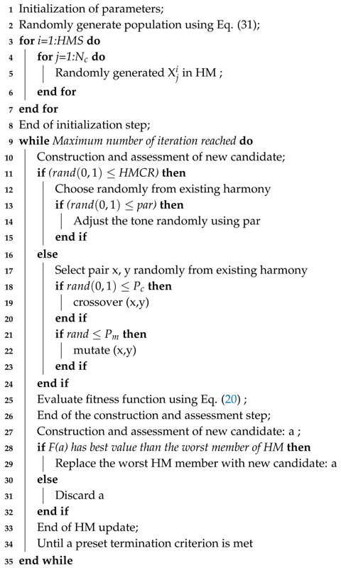
Initially, GHSA has followed the same steps as the steps of HSA. Equation (
31) generates the random values using parameters given in
Table 6. The newly generated values are stored and named as harmony memory (HM). HM is binary coded string showing the ON and OFF status of the appliance. After defining HM using Equation (
32) the improvisation of HM is done by generating a new harmony vectors based on HMCR using Equation (
33). The selected candidate is further modified according to Par. Par calculates the probability of the candidate from HM to be modified and (1-Par) probability of doing else as in Equation (
34). However, up to this step, the results achieved by HSA are restricted to only a particular region and the dynamic capability in search of global optimal solution is also confined. In order to overcome this issue, the stochastic operators of GA are introduced i.e., crossover and mutation. These operators not only improve the diversity of the solution but also help to provide higher efficiency towards an optimal solution. As a result, the modified hybrid algorithm GHSA effectively achieve the optimum solution with the faster convergence rate and hence give better results than other algorithms. Therefore, the stochastic operators are employed and the fitness function is evaluated using Equation (
20). This new value of the harmony is compared with existing worst harmony in HM and the worst harmony is excluded. The process continues until the termination criteria is met.
The computational time of proposed and existing algorithms for SH and MHs is given in
Table 7 and the Algorithm 1 shows working steps of the proposed algorithm GHSA.
2.10. Feasible Region
Feasible region is defined as the set of optimal points which satisfies all the constraints given in a scenario, including inequalities, equalities, and integer constraints. We consider feasible region of electricity cost versus energy consumption and electricity cost versus for a SH and MHs using RTEP and CPP tariffs.
2.10.1. Feasible Region for SH
In this segment, we figure out the feasible region for electricity cost and energy consumption of SH by considering RTEP and CPP tariffs. Firstly, we consider a SH with RTEP tariff and the electricity cost per hour is given:
Similarly, the total electricity cost is calculated as:
| Algorithm 1: GHSA |
![Energies 11 00190 i001]() |
To minimize Equation (
36), we introduce constraints regarding RTEP tariff and energy consumption of the appliances are:
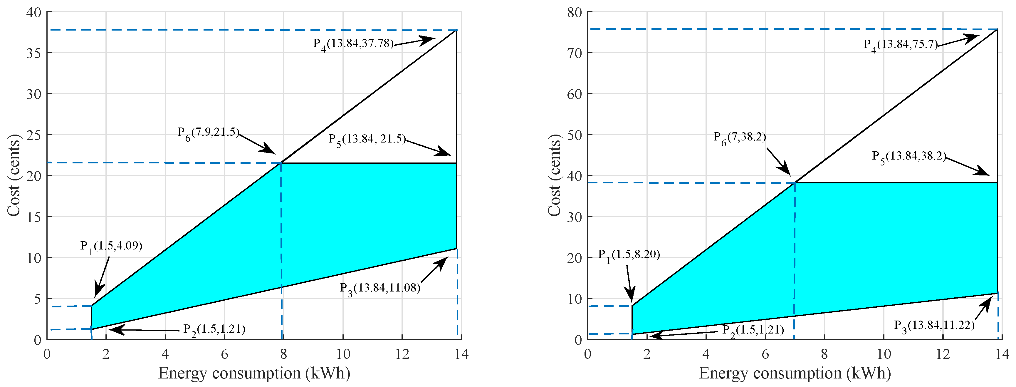
In
Figure 2a points P
, P
, P
, P
, and P
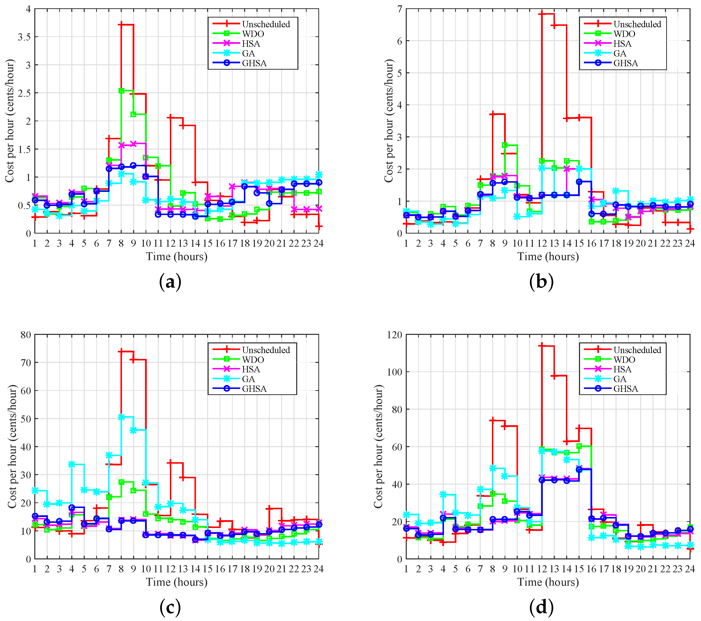
show the feasible region of electricity cost and energy consumption. The electricity cost is calculated using RTEP tariff and the unscheduled cost per hour is 3.71 cents. The total cost per day is 21.6 cents and based on the parameters electricity cost and energy consumption the constraints are defined. The constraint
shows that the electricity cost in hour should not exceed 3.71 cents including peak hours and off-peak hours. Constraints
shows total cost per day should not increase than the 21.5 cents as total cost shown here is in the unscheduled case, therefore, the scheduling algorithms must schedule the cost in such way that it should not exceed the limit as in
. While the constraint
shows the total energy consumption of the appliances must be with in limits i.e., between 1.5 and 13.84 kWh to reduce electricity cost. Similarly,
Figure 2b shows feasible region for SH considering CPP tariff and the constraints are given as:
Constraints associated with CPP show that the electricity cost of an hour should not exceed 6.37 cents. Constraint shows the cost for a single day should be less than 37.5 cents. While the constraint shows for the optimal scheduling of the energy consumption, energy consumed in an hour should be with in limits of 1.5 kWh and 13.84 kWh.
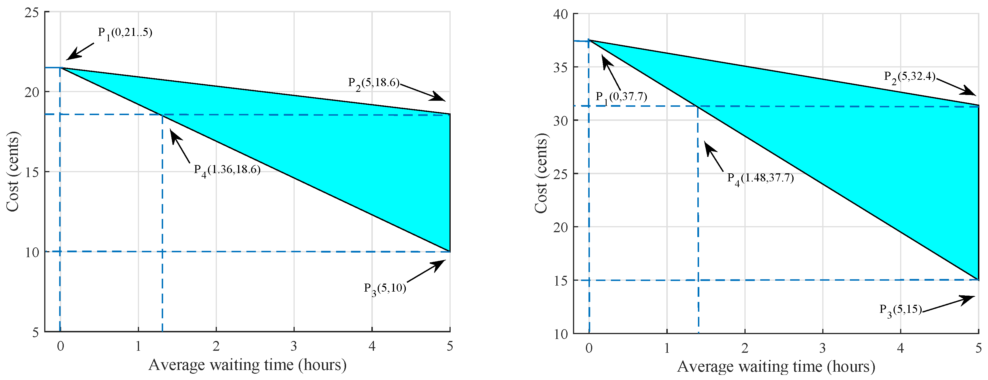
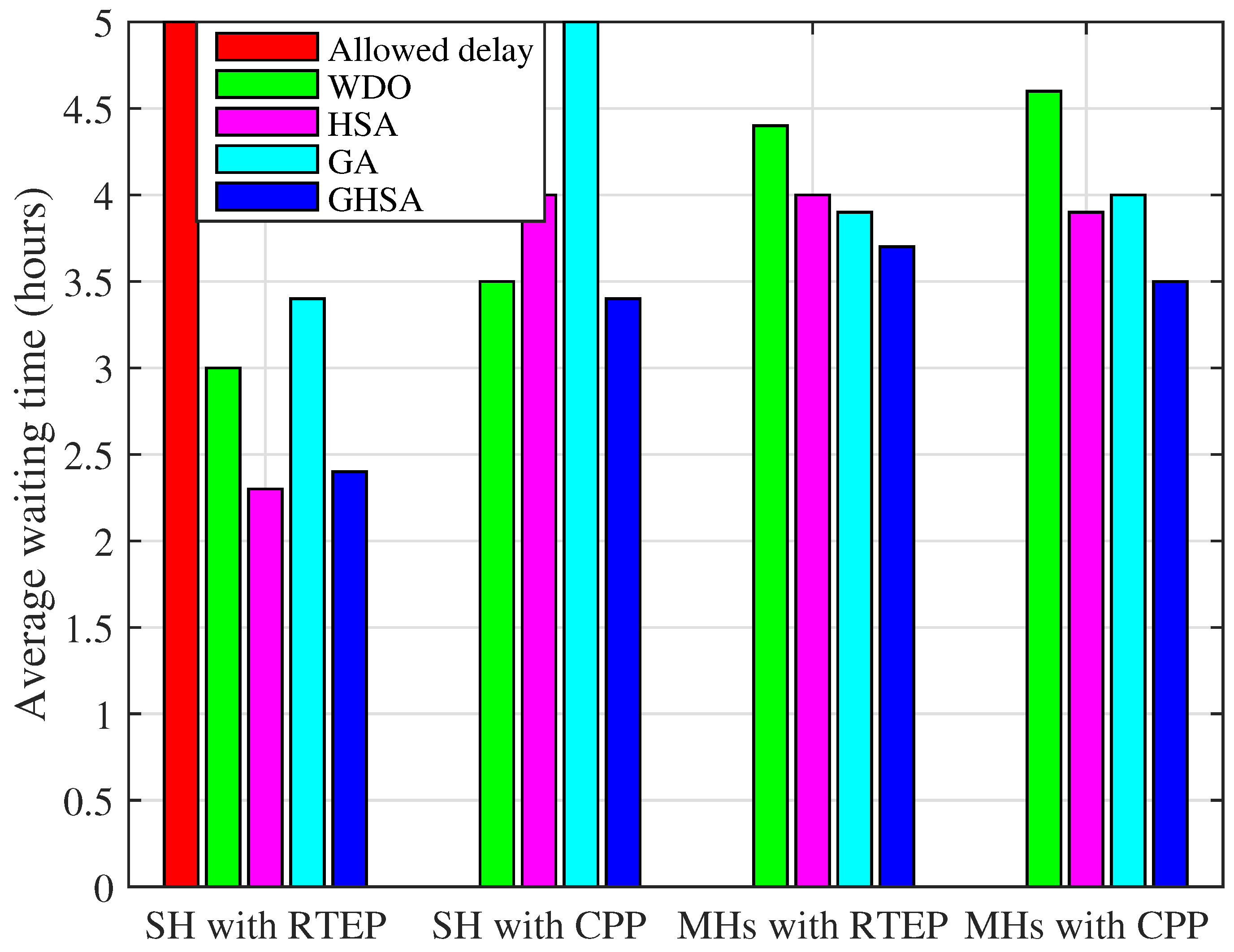
We also computed feasible region for electricity cost and
of the appliances in order to determine the user comfort. User comfort is inversely related with the
of the appliances and electricity cost. We consider maximum value of
is 5 h for the appliances i.e., allowable delay for the operation of the appliances. In
Figure 3a points P
, P
, and P
show the feasible region for electricity cost and
using RTEP tariff. The point P
shows that the
of the
and
are restricted to zero, then the electricity cost is reached to a maximum value i.e., 21.5 cents whereas, point P
shows the
of
is 5 h then the cost is reduced to 18.6 cents. While point P
shows that
of all the appliances, including
and
is 5 h then the cost is reduced to 10 cents, however, in this case consumers have to pay less cost, but compromise its comfort level. Similarly, in
Figure 3b point P
shows that the consumers have to pay maximum cost 37.7 cents when
is zero. Whereas, point P
shows that the cost is reduced to 18.6 cents when the
of the
is 5 h. While point P
presents that the cost is decreased to 15 cents as the
of the appliances is increased to 5 h. The feasible region of
Figure 3a,b depicts the trade-off between the electricity cost and
of the appliances. In order to minimizes the trade-off optimal scheduling of the energy consumption profile is essential in peak hours and off-peak hours.
2.10.2. Feasible Region for MHs
The feasible region of electricity cost and energy consumption for MHs is determined using RTEP and CPP tariffs. Similar to previous segment, we consider MHs using RTEP and CPP tariffs and the total cost is calculated as:
Constraints associated with electricity cost and energy consumption for MHs using RTEP are given as:
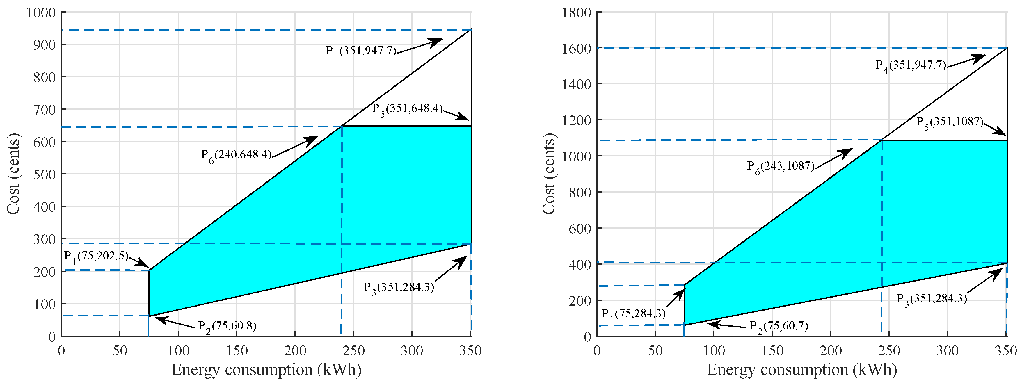
In
Figure 4a the shaded region shows the feasible region of electricity cost and energy consumption of MHs using RTEP tariff. Constraint
indicates the cost per hour must be restricted with in limits of 50.6 and 94.4 cents. While the cost per day is restricted to 648.43 cents by the constraint
. Constraint
presents that the energy consumption should not exceed upper and lower bound i.e., 75 and 351 kWh respectively.
Figure 4b shows the feasible region of the electricity cost and energy consumption for MHs using CPP tariff. The constraints related to electricity cost and energy consumption for MHs using CPP are:
Similar to prior constraints, the constraint indicates that electricity cost in an hour should be restricted by upper and lower bound i.e., 58.7 and 156.8 cents, respectively. Constraint shows that heuristic algorithm should schedule the cost such that it should not increase 1087 cents. While constraint simply means that for minimization of electricity cost energy consumption of the appliance should not exceed the given values as in .
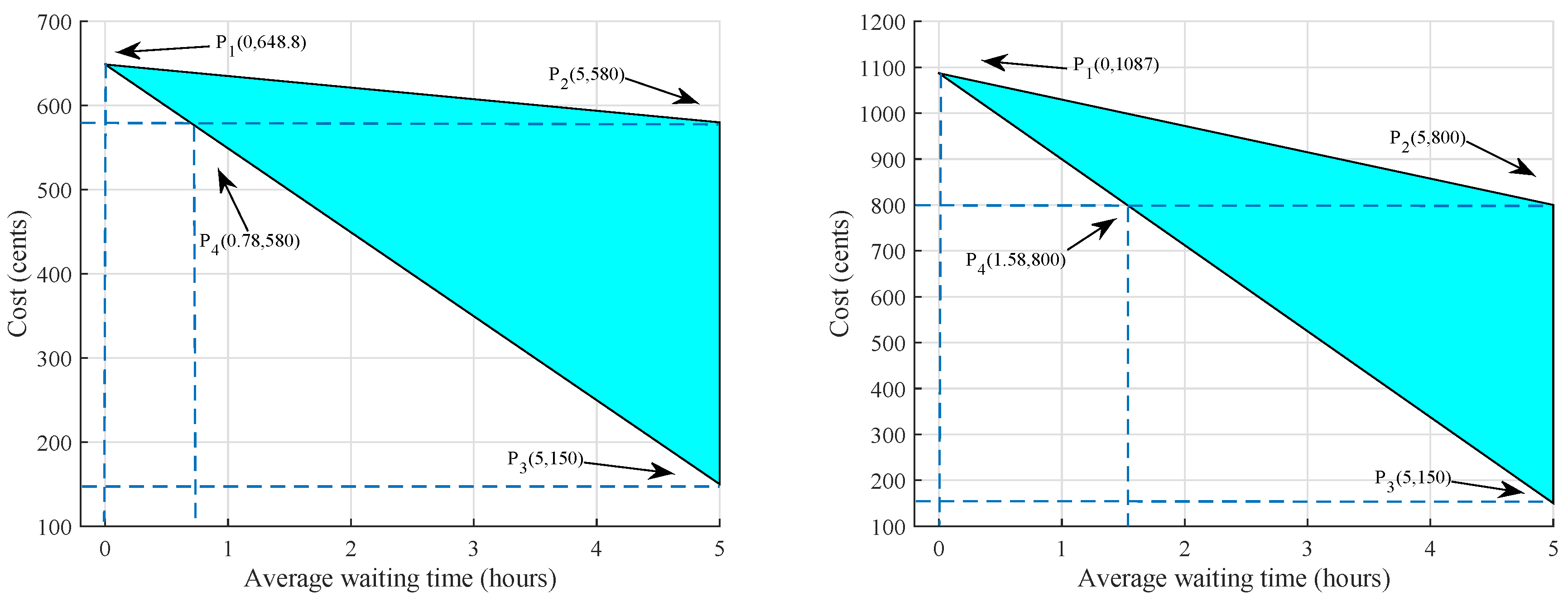
In
Figure 5a points P
, P
, and P
illustrate the feasible region of electricity cost and
of MHs using RTEP tariff. The point P
shows that the electricity cost is maximum when
is zero, while point P
represents that at the maximum value of the
of the appliances the total cost is minimum i.e., 150 cents. However, at this stage user comfort is decreased. P
shows the cost is reduced to 580 cents when the operation time of
is delayed to its maximum value i.e., 5 h. Similarly,
Figure 5b shows the feasible region bounded by the points P
, P
, and P
with CPP tariff. The maximum cost in case of CPP is raised to 1087 cents at zero
. Whereas, P
shows the cost when the operation time of
is delayed only. While P
shows that
is maximum for all the appliances the cost is minimum i.e., 150 cents. Moreover, to address the trad-off in a better way, it is important to consider electricity cost and user comfort equally and appropriately.
4. Conclusions and Future Work
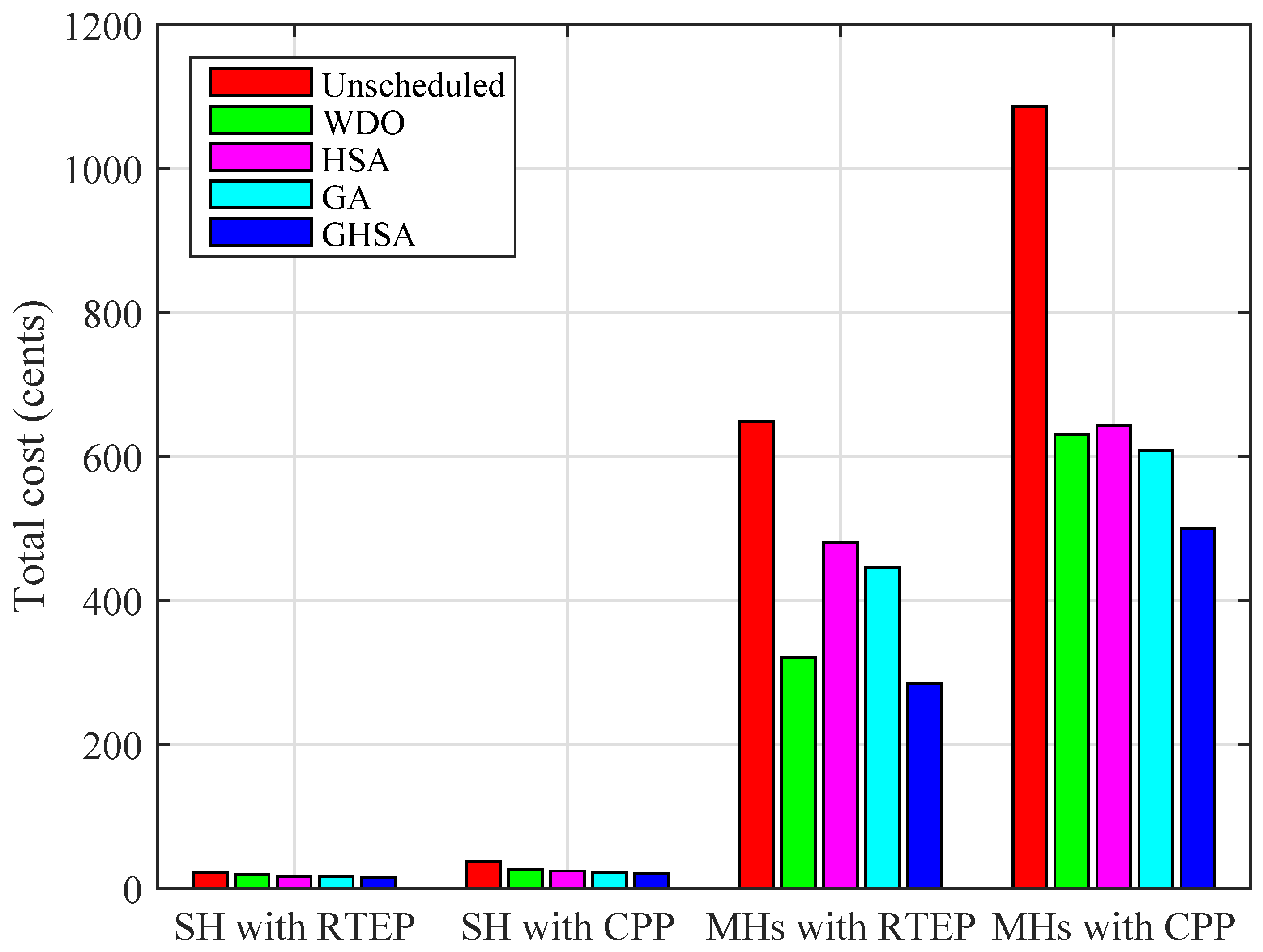
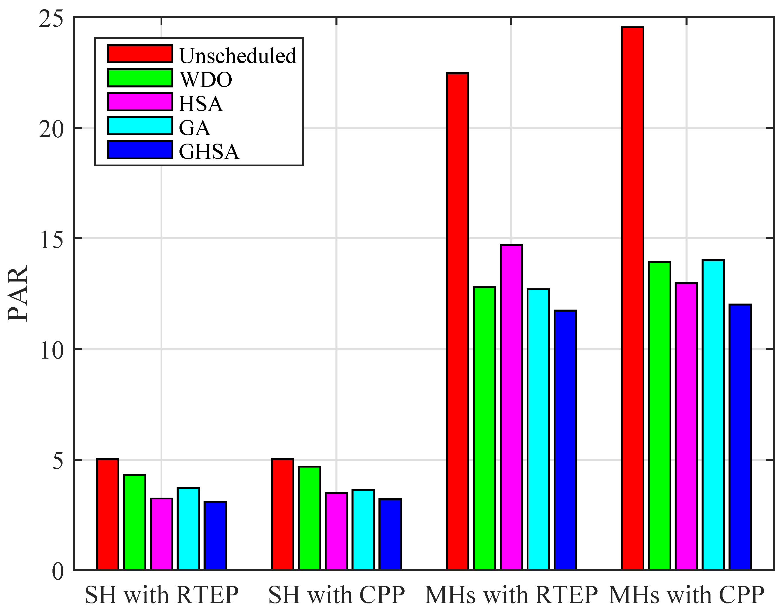
In this paper, we have proposed a heuristic algorithm GHSA for SH and MHs to reduce electricity expense, PAR, and maximize user comfort. The proposed algorithm is tested in the presence of RTEP and CPP tariffs for SH and MHs. In case of MHs, arbitrary power ratings and time of operations are assigned to the appliances. Extensive simulations are conducted which show the performance of proposed algorithm GHSA is efficient as compared to existing algorithms: WDO, HSA, and GA in terms of electricity cost, PAR, and user comfort. In particular, GHSA reduces the electricity cost to 46.19% in case of SH. While for MHs the electricity cost is reduced to 56.04%. In terms of PAR, GHSA reduces PAR to 38.32% and 50.08% for SH and MHs, respectively. The minimization in electricity cost and PAR reveal benefits to the consumers as well as improve the stability and reliability of the power grid. Moreover, feasible regions are computed to validate the effectiveness of our proposed algorithm GHSA. Thus, it is concluded from above discussion that the proposed EHEMC based on GHSA yields significantly improved performance as compared to existing heuristic algorithms in terms of electricity cost, PAR and user comfort.
In future, we are interested to implement the integration of RESs for both cases i.e., SH and MHs. We are also interested to incorporate distributive algorithms and multi objective problems with convex optimization methods.

 ,
, 


