Study on the Effect of Reciprocating Pump Pipeline System Vibration on Oil Transportation Stations

Abstract

Due to the periodic movement of the piston in the reciprocating pump, the fluid will cause a pressure pulsation, and the resulting pipeline vibration may lead to instrument distortion, pipe failure and equipment damage. Therefore, it is necessary to study the vibration phenomena of reciprocating pump pipelines based on pressure pulsation theory. This paper starts from the reciprocating pump pipe pressure pulsation caused by a fluid, pressure pulsation in the pipeline and the unbalanced exciting force is calculated under the action of the reciprocating pump. Then, the numerical simulation model is established based on the pipe beam model, and the rationality of the numerical simulation method is verified by indoor experiments. Finally, a case study is taken as an example to analyze the vibration law of the pipeline system, and vibration reduction measures are proposed. The following main conclusions are drawn from the analysis: (1) unbalanced exciting forces are produced in the elbows or tee joints, and it can also influence the straight pipe to different levels; (2) in actual engineering, it should be possible to prevent the simultaneous settlement of multiple places; (3) the vibration amplitude increases with the pipe thermal stress, and when the oil temperature is higher than 85 °C, it had a greater influence on the vertical vibration amplitude of the pipe.

1. Introduction

At present, oil is still the mainstream of the energy industry, and pipelines are the main way of oil transportation. Therefore, the safe operation of pipelines is the key to ensure the transportation of oil products, and is also the key to guarantee the normal operation of other industries. Strong vibrations of the pipeline will not only expose the structure of the pipeline and its pipe parts to fatigue damage, causing connection parts to loosen and rupture, measuring instrument distortion or even damage, but also cause noise pollution, which can affect the staff’s physical and mental health. Excessive vibration may even cause serious accidents and cause significant economic losses, affect the transport efficiency of oil products, cause great energy losses, and perhaps seriously pollute the environment. According to a Canadian expert, in industrially developed America, the losses caused by pipe vibration in the past amounted to more than $10 billion annually, and in 100 cases of damage incidents, pipeline vibration factors accounted for 19% [1,2]. Therefore, vibration analysis is necessary before pipeline systems with reciprocating pumps are put into operation. This area of research has important engineering significance to ensure the safe and stable operation of pipelines in oil stations.

Within one and a half years, 18 failures occurred in the pipes of the Dina pumping station in Columbia (Republic of Colombia), where the failures were caused by vibration [3]. In March 2006, the export valve of a hydrogen compressor in a Chinese enterprise suddenly fell off due to vibration, causing a large scale flammable and explosive gas leak, that eventually exploded [4]. On the contrary, the Benxi chemical fertilizer plant solved the problem of pipeline vibration of a compressor in 1984, any the safety has been guaranteed since. Besides, an increase of gas transmission efficiency and a reduction of power consumption were achieved [5].

Pipeline vibration research can be traced back to 1950s, when the KBR (Houston, TX, USA) company studied pipeline vibration problems, although they failed to vigorously promote the development of this problem because the conditions and methods were immature [6]. In 1975, Bickford et al. used the transfer matrix method to analyze the vibration problem of plane beams [7]. In 1976, Paidoussis and Laithier took a short pipe as a Timoshenko beam and studied its stability. It is found that the beam model is not suitable for the short pipe because pipe has both beam vibration mode and shell vibration mode [8]. In 1980, Irie et al. deduced a transfer matrix method for analyzing the vibration stability of pipelines [9]. In 1990, Lesmez et al. first used the separation of variables method in the derivation of the transfer matrix of a space complex pipeline system. This method is more flexible and can solve the vibration problem of complex space pipeline systems [10].

In the aspect of pipeline modeling, usually a beam model or shell model is used. The beam model is mainly applied to the cases where the pipe is much longer than the pipe diameter, and the shell model is more suitable for the local analysis of the pipeline. Researchers have studied the beam model more extensively. Ashley used the beam model to study the theory and experiment of pipeline vibration [11]. Fuller and Fahy used single-frequency and axial single-point excitations to study the vibration of forced vibration straight pipes, and achieved numerous useful results [12]. Adachi et al. used a complete shell model to analyze the vibration of straight pipes, and compared the results with other scholars’ calculations. It was concluded that the shell model was suitable for the pipes which are extremely short or when accurate results are needed. After using the beam model, the Dunkerley method and the Ritz method can be used to calculate the natural frequency of the pipeline. For the complex pipe system, the finite element method and the transfer matrix method are always used [13].

In the aspect of pipeline vibration reduction, in 2007, Yu et al. analyzed the vibration and vibration reduction measures of reciprocating compressor pipelines. Moreover, some measures such as increasing the buffer tank, changing the diameter and so on were put forward [14]. In 2009, Ye used the ANSYS (Canonsburg, PA, USA) software to analyze the vibration of water injection pump pipelines in oil fields [2]. Also in 2009, Chen used the electro-acoustic analogy method which regards a pipe unit as a circuit to analyze the vibration of pipelines in reciprocating compressor systems; this method is convenient and fast, but it can only be used to calculate the frequency of the pipeline [6]. In 2011, Zhou et al. used the separation of variables method to deduce the expression of pressure pulsation [15].

From the literature, it can be seen that in recent years most of the research on pipelines with reciprocating equipment are focused on the pipeline frequency. Moreover, vibration reduction studies are mainly from the point of natural frequency enhancement and pressure pulsation control, and the studies did not start with the amplitude of the pipeline. Pressure pulsation calculations can be divided into analytical methods and finite element methods. Although the pressure pulsation can be calculated by the analytical method, the pressure non-uniformity cannot reflect the real situation. The finite element method needs to use other professional software such as PRO/ENGINEER (Parametric Technology Corporation, Boston, MA, USA), making its modeling process more cumbersome.

One of this paper’s authors, Lu, did a similar study in 2016 [16], but that paper was only from the point of view of pipeline stress and vibration frequency. Moreover, that paper did not compare the amplitude difference between the static condition and pressure pulsating condition. In this paper, numerical simulation combined with experimental methods were used for reciprocating pump pipeline vibration analysis. Firstly, the vibration analysis method of a reciprocating pump is established based on the pressure pulsation theory, a simple pipeline is designed, and the analytical method is verified by indoor experiments. Secondly, this verified method is used to analyze the vibration of the actual pipeline of an oil station and measures for vibration reduction are put forward.

2. Theory

The vibration analysis of the reciprocating pump pipeline is performed usually in accordance with the process shown in Figure 1. Therefore, the basic theories involved include: the calculation of the pressure pulsation, the calculation of the unbalanced exciting force, and the modeling of the pipeline.

2.1. Pressure Pulsation

Pressure pulsation refers to the maximum amplitude deviation from the average pressure. In the case of absence of actual pipeline pressure field data, it is difficult to calculate by shock-wave theory, so in order to ensure the results’ accuracy, the separation of variables method is used [15,17,18].

The expression of pressure pulsation is:

$$p_{\Delta }\left(x,t\right)=\left[\frac{-2p}{n\pi }\left(\cos n\pi l-1\right)\cos {\omega }_{n}t+\frac{-2u}{n^2{\pi }^{2}cl}\left(\cos n\pi l-1\right)\sin {\omega }_{n}t\right]\sin \frac{n\pi }{l}x$$

(1)

where p_Δ(x,t) is the pressure pulsation at x position and t time (in Pa); n is the order number; c is sound velocity (m/s); l is total pipe length (m); x is distance from the starting point (m); ω_n is excitation circular frequency (rad/s); p is initial pressure (Pa); u is initial velocity (m/s).

2.2. Unbalanced Exciting Force

The reciprocating pump produces a pressure wave in the pipe at a regular time interval. The pressure wave propagates through the fluid and produces harmonic loads at each elbow in the pipe system, as shown in Figure 2. It is assumed that the inner diameter of the pipe is d_i, the angle of elbow is β, the inlet and outlet pressures are p, then the resultant force of elbow is [15,19,20]:

$$R=2F_1\sin \left(\frac{\beta }{2}\right)=2F_2\sin \left(\frac{\beta }{2}\right)=2\left(\frac{\pi d_i^{2}p}{4}\right)\sin \left(\frac{\beta }{2}\right)$$

(2)

If p is constant, then R is constant and the bend deformation and stress are static. If the pressure is pulsating, then p = p₀ + Δp and the resultant force of elbow is:

$$R=2\left(\frac{\pi d_i^2}{4}\right)\left(p_0+\Delta p\right)\sin \left(\frac{\beta }{2}\right)=2\left(\frac{\pi d_i^2}{4}\right)p_0\sin \left(\frac{\beta }{2}\right)+2\left(\frac{\pi d_i^2}{4}\right)\Delta p\sin \left(\frac{\beta }{2}\right)$$

(3)

where p₀ is average pressure, Pa; Δp is amplitude of pressure pulsation, Pa.

In Equation (3), the first term is the force produced by static pressure on the elbow, the second term is the alternating force—ΔR—produced by pressure pulsation:

$$\Delta R=2\left(\frac{\pi d_i^2}{4}\right)\Delta p\sin \left(\frac{\beta }{2}\right)=2S\Delta p\sin \left(\frac{\beta }{2}\right)$$

(4)

where Δp is pressure pulsation, Pa; S is cross sectional area of pipe, m².

From Equation (4), it can be seen that the exciting force of the pipe increases with the increase of the elbow angle when the pulsating pressure is constant within a 0–180 degree range of the elbow angle.

2.3. Pipeline Model

The pipeline model section mainly includes the mechanical model of the pipeline, the finite element mesh and the finite element method of the pipeline structure. These contents are available in two additional papers published by author Lu [5,16].

3. Numerical Simulation Method and Verification

3.1. Numerical Simulation

Because the pipeline of a reciprocating pump is more complex, the pipe beam model is usually used. Compared with ANSYS, ABAQUS (SIMULIA, Johnston, RI, USA) and other finite element analysis software, the CAESAR II (Intergraph, Huntsville, AL, USA) software is simpler to operate and quicker in calculation speed, and the accuracy can meet engineering requirements, making it especially suitable for mechanical calculations of complex piping systems. The following assumptions are made for the calculation of the vibrations of the reciprocating pump pipelines using the CAESAR II software:

(1)

The small deformation assumption is that the local deformation of the cross-section of the element under load is negligible;

(2)

The pipe material is in the elastic range without considering the plastic deformation and large deformation, that is, the nonlinear nature of the pipe structure is not considered;

(3)

The plane stays flat during loading;

(4)

We only consider the elastic changes of the pipe and the load, i.e., Hooke’s law applies to the full load range of the tubular section;

(5)

The forces and moments acting on the structure are assumed to be the points acting on their central axes;

(6)

The amount of rotational deformation of the system is assumed to be small;

(7)

The force is not affected by structural deformation;

(8)

We ignore the friction between the liquid and the pipe wall;

(9)

There is no vacuolization in the liquid filled pipeline [5].

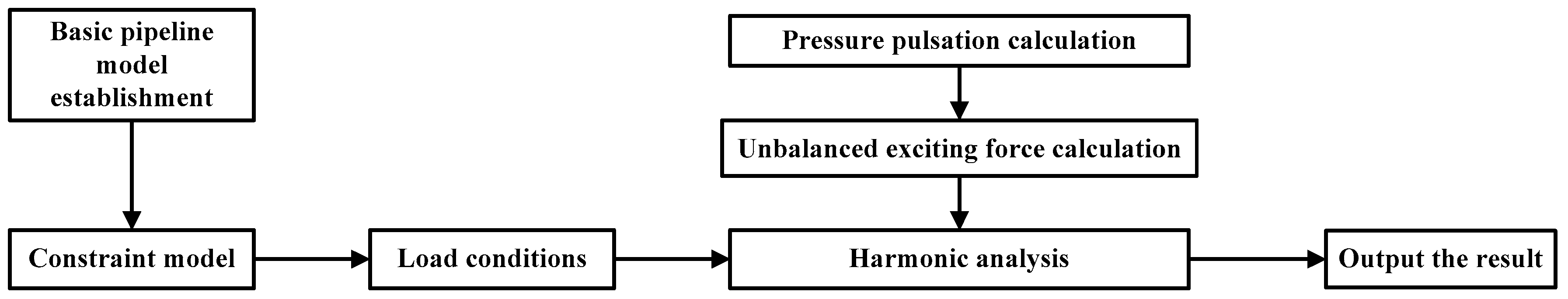
The vibration analysis of pipes is usually done according to the process shown in Figure 1, and the corresponding numerical simulation steps are as follows: (1) establish a pipeline foundation model: input the basic parameters of the pipeline such as inner pressure, thickness, pipe material, not including pipeline constraints; (2) establish the constraint model according to the actual engineering loads or constraints; (3) set the load condition: combine the load according to the actual pipe load, such as pressure, temperature; (4) harmonic analysis: call harmonic analysis module in CAESAR II software and enter the unbalanced exciting force calculated from Equation (4).

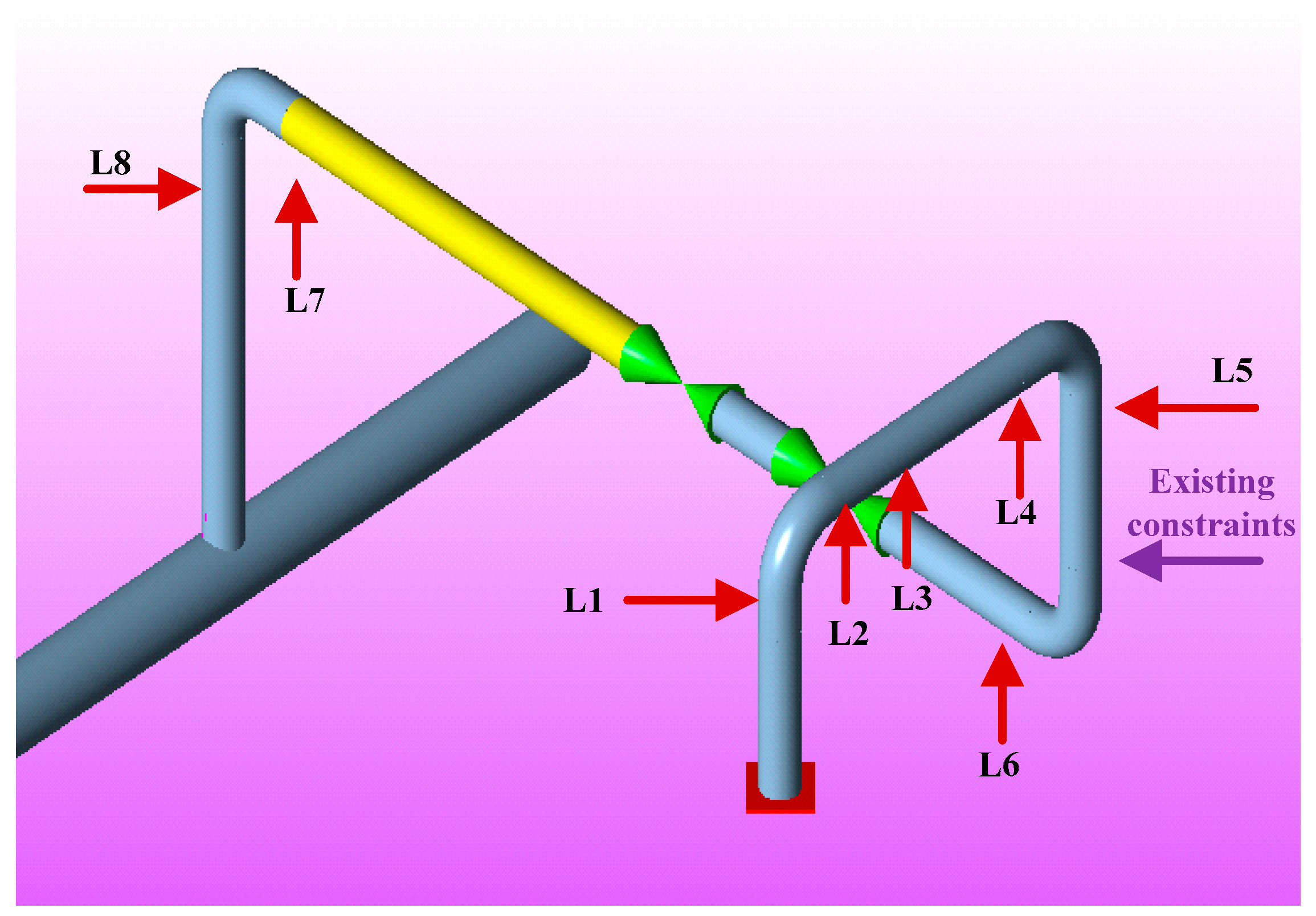
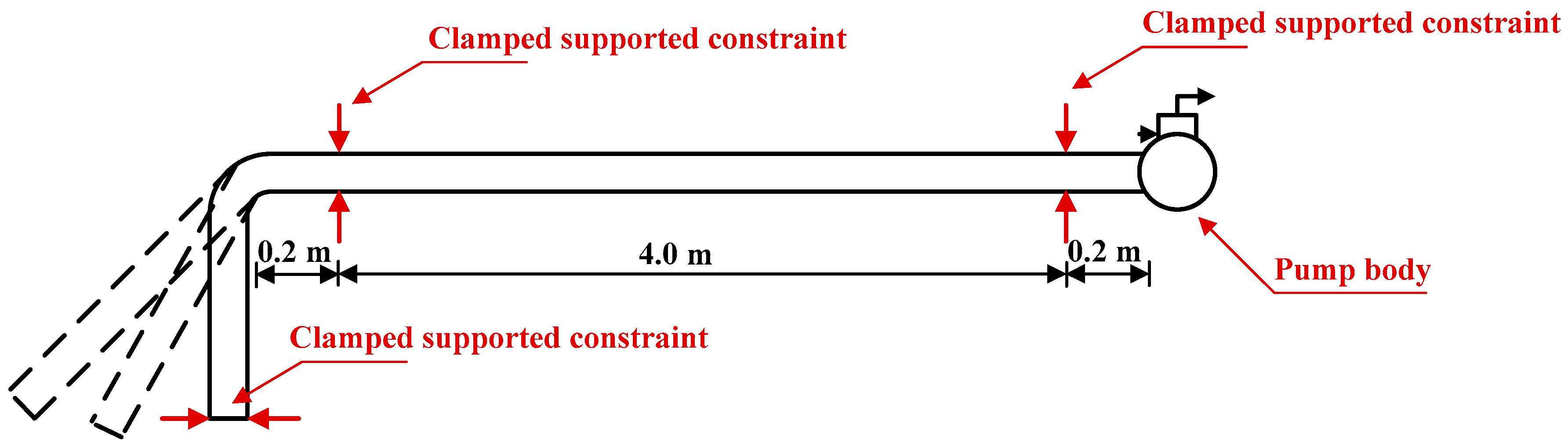
In order to verify the correctness of the numerical simulation method, this method is used to simulate a simple pipeline and is verified by indoor experiments. As shown in Figure 3, the simple pipe model is divided into a straight pipe section and an elbow section, wherein the straight pipe section is 4.4 m long, and the angle of the elbow is set at 90 60 and 45 degrees. The direction of fluid flow in the pipeline is from right to left. There are three clamped supported constraints in the pipeline, and the specific parameters of the pipeline are listed in

Table 1. Pipeline material parameters and structural parameters.

Items	Parameters	Straight Pipeline	Elbow
Structural parameters	Outside diameter D	33.5 mm	33.5 mm
	Pipeline thickness ξ	2.5 mm	2.5 mm
	Curved radius of elbow R	-	120 mm
	Straight pipe length at both ends of the elbow l	-	340 mm
	Straight pipe length L	4000 mm	-
Material parameters	Pipeline material	Q235 galvanized pipe
	Minimum yield strength	235 MPa
	Modulus of elasticity E	206 GPa
	Density ρ	7860 kg/m3
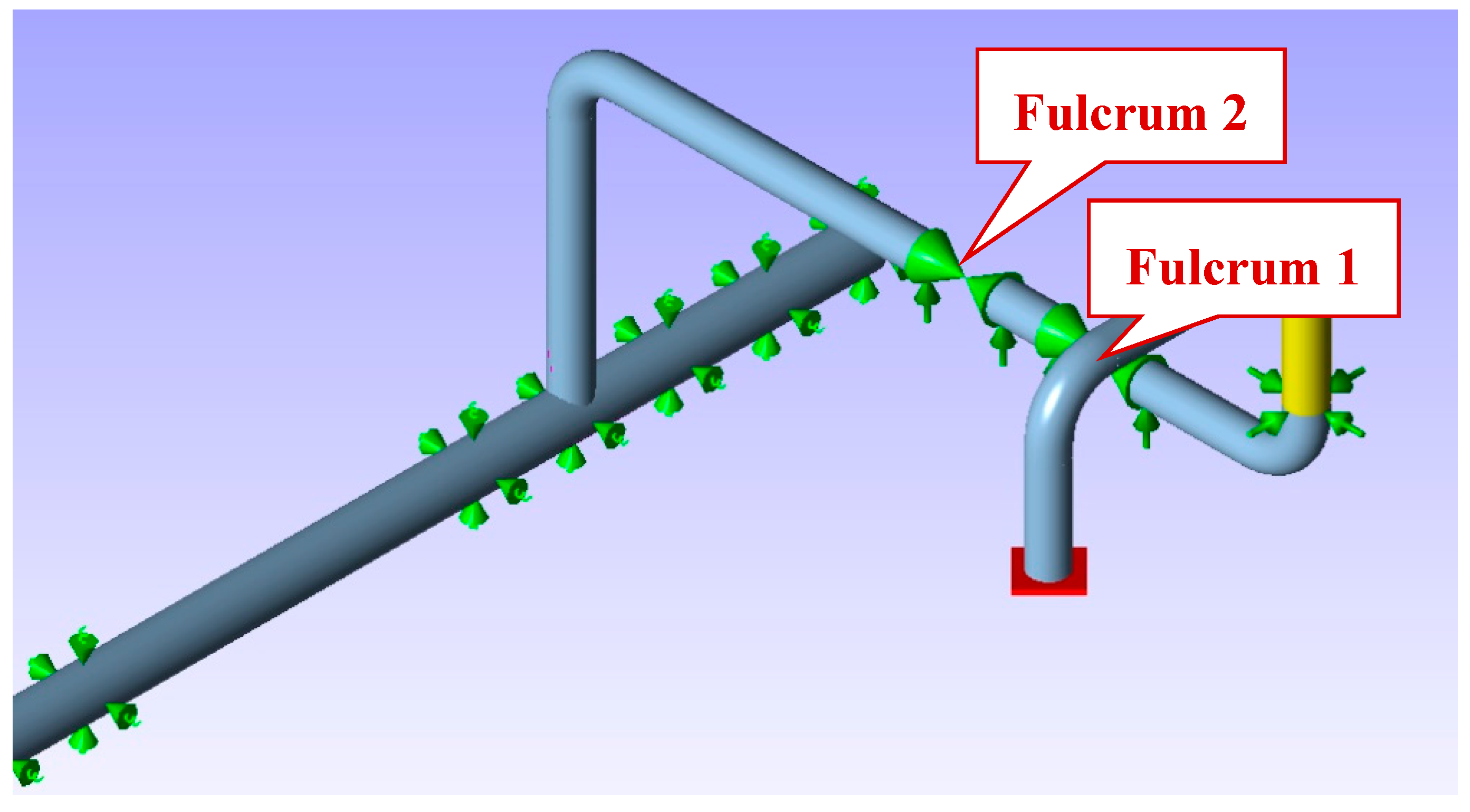
	Poisson ratio ε	0.3

. The pump delivery pressure is 0.9 MPa, the transmission medium is water, the temperature is 15 °C, and the inlet flow rate is 1283 L/h. Pipeline foundation model and constraint model can be seen in Figure 4.

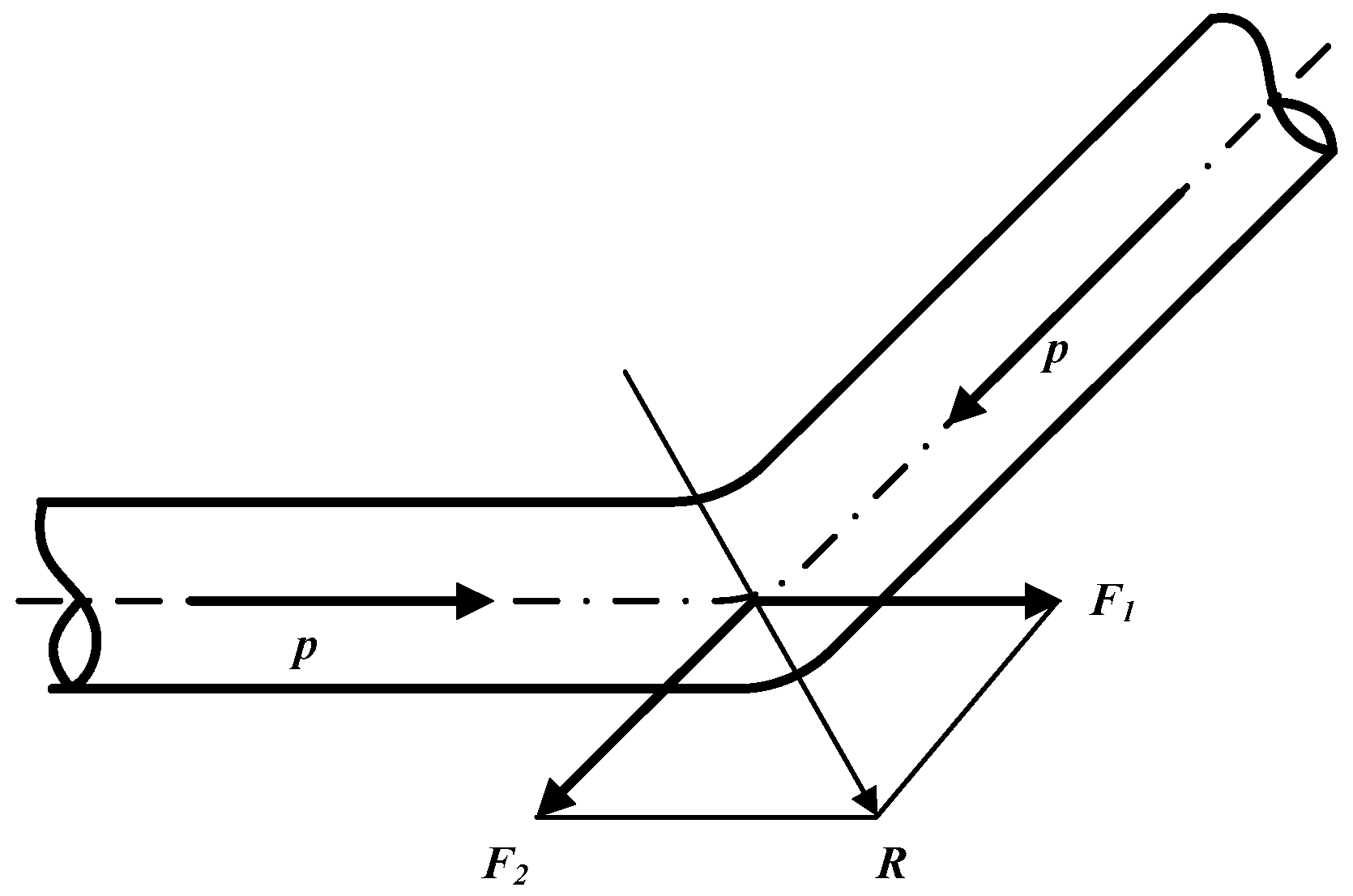
The unbalanced exciting force of the elbow is calculated as follows:

The pump revolution speed is 170 r/min, it belongs to single cylinder single-action equipment, and then the excited frequency is:

$$f=nNP/60=170÷60=2.83\mathrm{Hz}$$

Circular frequency is: $\omega =2\pi f=2\times 3.14\times 2.83=17.77\mathrm{rad}/\mathrm{s}$

Sound velocity is: $c=\sqrt{\frac{E_{water}}{\rho }}=\sqrt{\frac{2.1\times {10}^9}{1000}}\approx 1449.14\mathrm{m}/\mathrm{s}$

The distance from the starting point to the elbow is 4.4 m, and the total length of the pipe is 5 m. The pressure pulsation at different times of the elbow can be calculated based on Equation (3):

Make x = 4.4 m, $t\in \left[0,200\right]$, n = 1, then Equation (3) can be written as:

$$p_{\Delta }\left(4.4,t\right)=\left[\frac{-2\times 0.9\times {10}^6}{\pi }\left(\cos 5\pi l-1\right)\cos 5.66\pi t+\frac{-2\times 0.56}{7245.7{\pi }^2}\left(\cos 5\pi -1\right)\sin 5.66\pi t\right]\sin \frac{4.4\pi }{5}$$

The calculated pressure pulsation of the first 100 s can be seen in Figure 5, it can be obtained that the maximum value of the pressure pulsation is 1031.00 Pa, and the minimum value of the pressure pulsation is −1030.71 Pa.

Then ΔP is: ΔP = 0.5(P_max − P_min) = 0.5 × (1031.00 + 1037.71) = 1031.36.

According to Equation (4), unbalanced exciting forces of 45 degree elbow, 60 degree elbow and 90 degree elbow are calculated:

45 degree elbow:

$$F=2\times \Delta P\times S\times \sin \left(\frac{45}{2}\right)=2\times 1031.95\times \frac{3.14\times {0.0285}^2}{4}\times 0.3827\approx 0.50\mathrm{N}$$

60 degree elbow:

$$F=2\times \Delta P\times S\times \sin \left(\frac{60}{2}\right)=2\times 1031.95\times \frac{3.14\times {0.0285}^2}{4}\times 0.5\approx 0.66\mathrm{N}$$

90 degree elbow:

$$F=2\times \Delta P\times S\times \sin \left(\frac{90}{2}\right)=2\times 1031.95\times \frac{3.14\times {0.0285}^2}{4}\times 0.707\approx 0.93\mathrm{N}$$

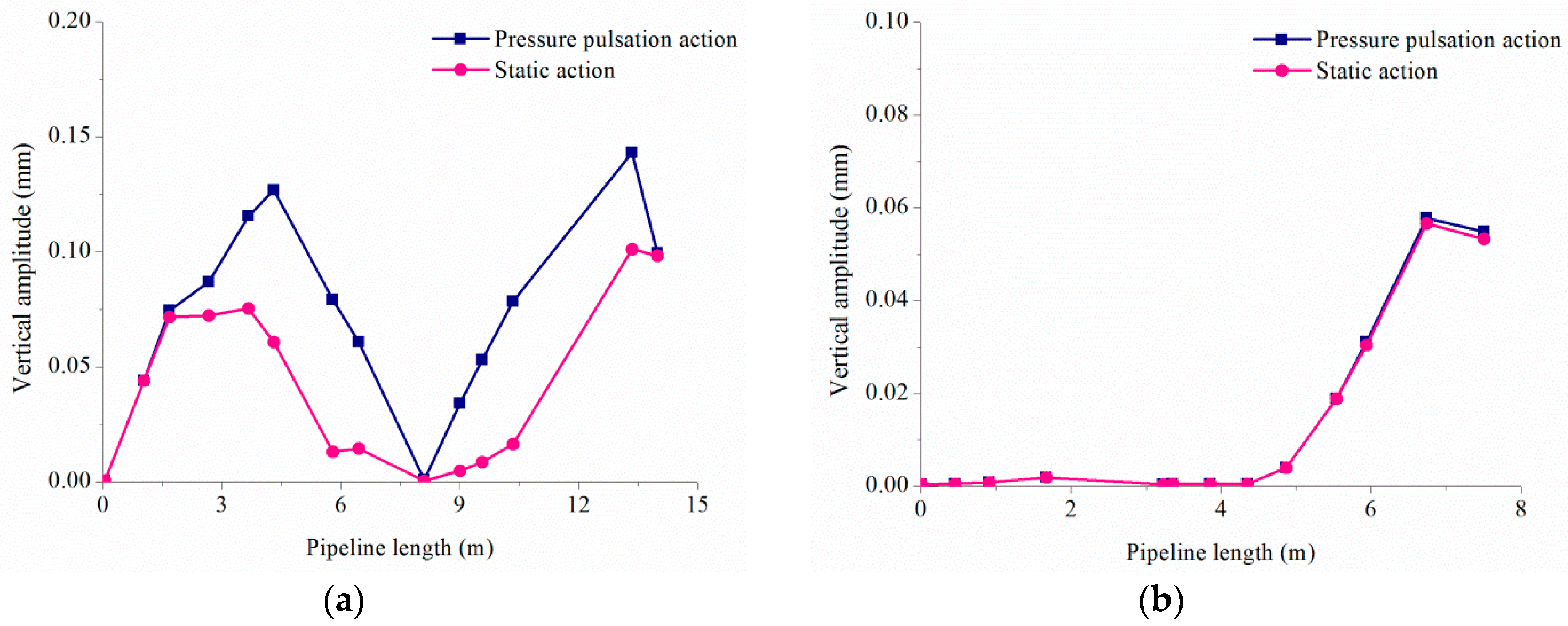
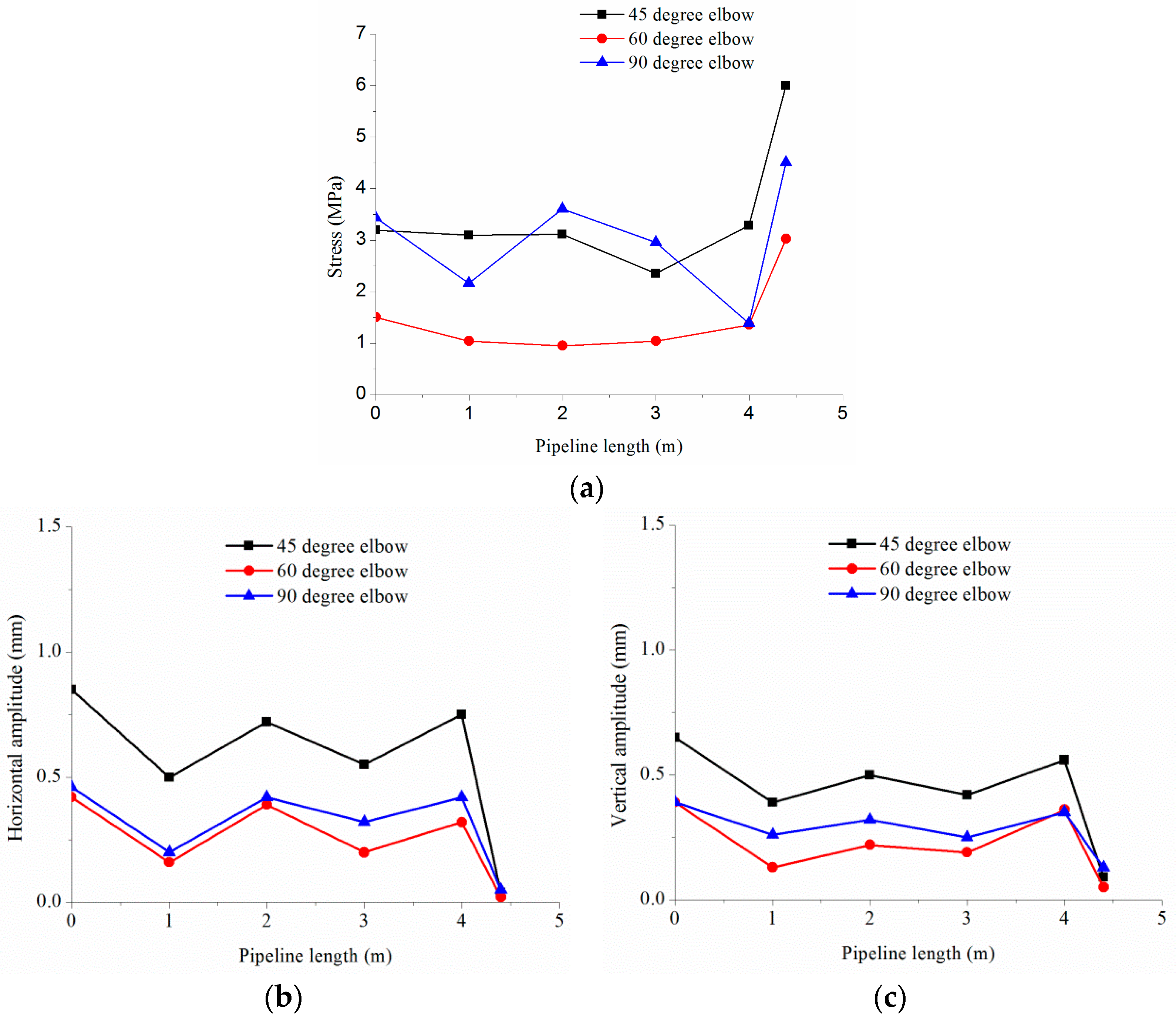
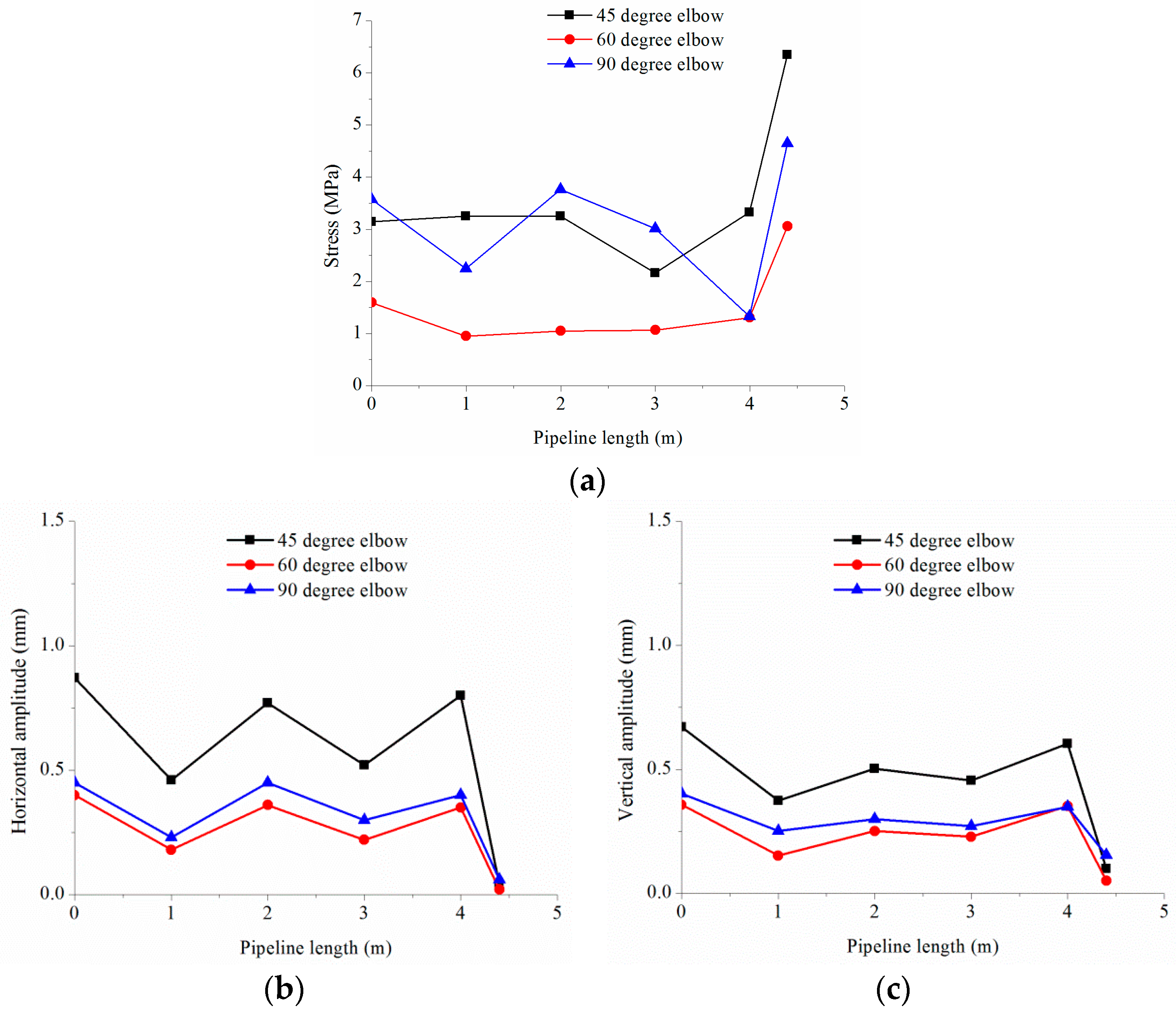
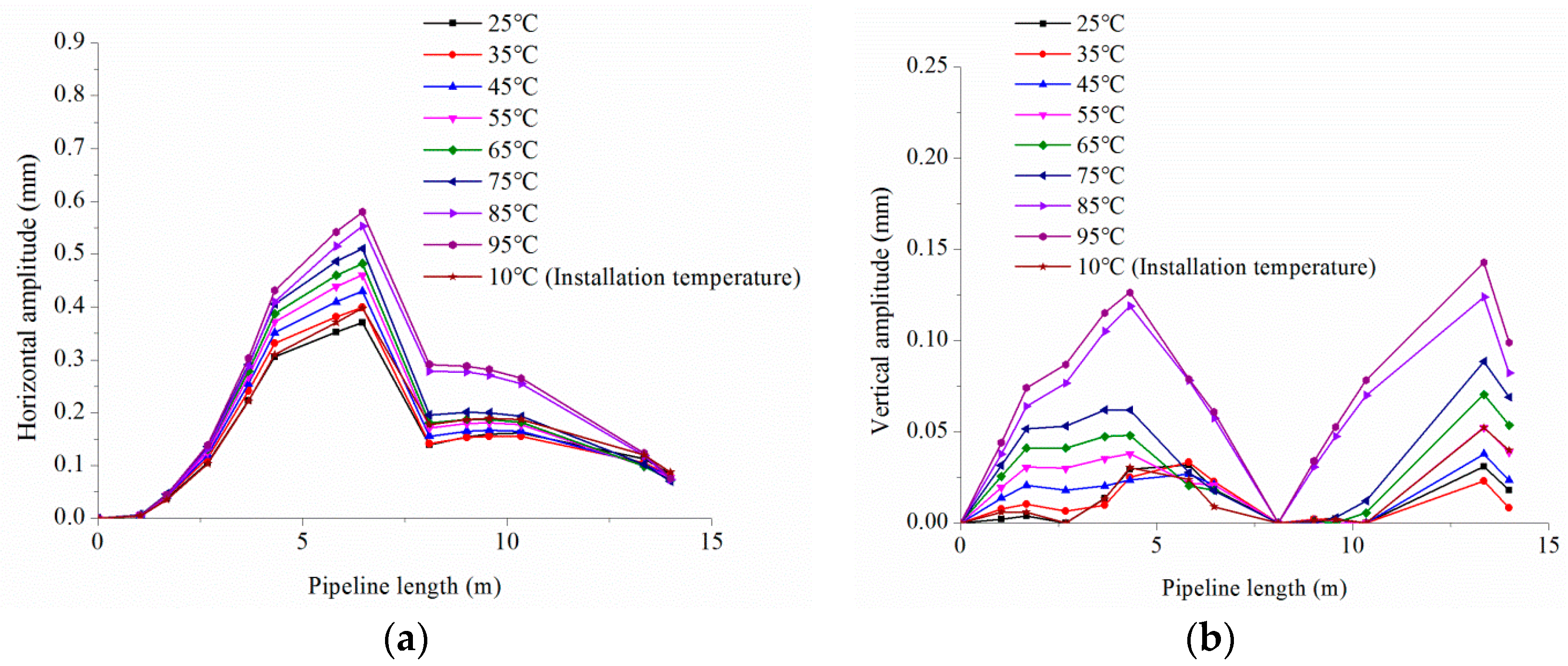
The calculated unbalanced exciting force is loaded onto the pipe, and the stress, horizontal and vertical amplitudes are computed by CAESAR II software. The results are shown in Figure 6.

3.2. Experimental Verification of Numerical Simulation Method

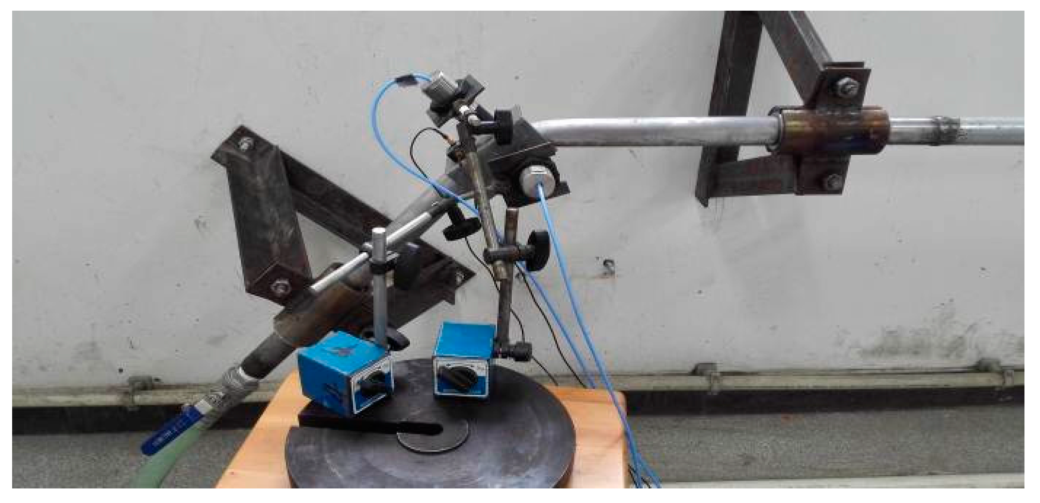
In order to verify the correctness of the numerical simulation method, an indoor experimental system is established according to the simple pipeline model used in numerical simulation. The experimental system is mainly composed of four subsystems, such as power unit, loop circuit, experimental platform and signal acquisition and analysis system. The main structure and composition are shown in Figure 7.

As shown in Figure 7, the straight pipe is connected with the elbow, and the axis of the straight pipe and the elbow are in the Z-Y plane. The piston pump provides a pulsating flow at different flow rates and pressures for the entire experimental system, the signal acquisition and analysis system (including strain gauges, acceleration and displacement sensors) measures the different test points of the test section under each operating condition.

There are three different elbow structures in the experiment: the elbow angles are 45°, 60°, and 90°, respectively. The inlet end of straight pipe and outlet end of elbow are connected by a flexible hose with an inner diameter of 25 mm, and fastened through the clamp. The fixed straight pipe section is connected with the two ends of the elbow through rigid band joints, so as to replace the elbow with different angles (as a result of the use of flexible hose, metering pump water flow will lead to flexible hose vibration, this vibration is inevitably passed to the test straight pipe, which belongs to the external excitation load, and has a certain influence on the straight section test data).

The experimental principle as shown in Figure 7, the elbow of test section is connected to a JD-1350/1.6-type plunger metering pump (pump maximum flow rate is 1350 L/h, the measurement accuracy is ±1%); the maximum pumping pressure is 1.6 MPa (accuracy: ±3%); the metering valve range is 1–100 mm (adjustment accuracy: 95%). The water flow through the metering pump from the water tank, through the LWGY-32 type turbine flow sensor (accuracy: ±0.5%R), a YB-2088 type pressure transmitter (accuracy: ±0.5%FS), transitional straight pipe with a length of 4 m (the material is the same as the elbow), elbow of test section, throttle valve and DN32 type rubber pressure-resistant steel pipe, then the water goes back to the water tank.

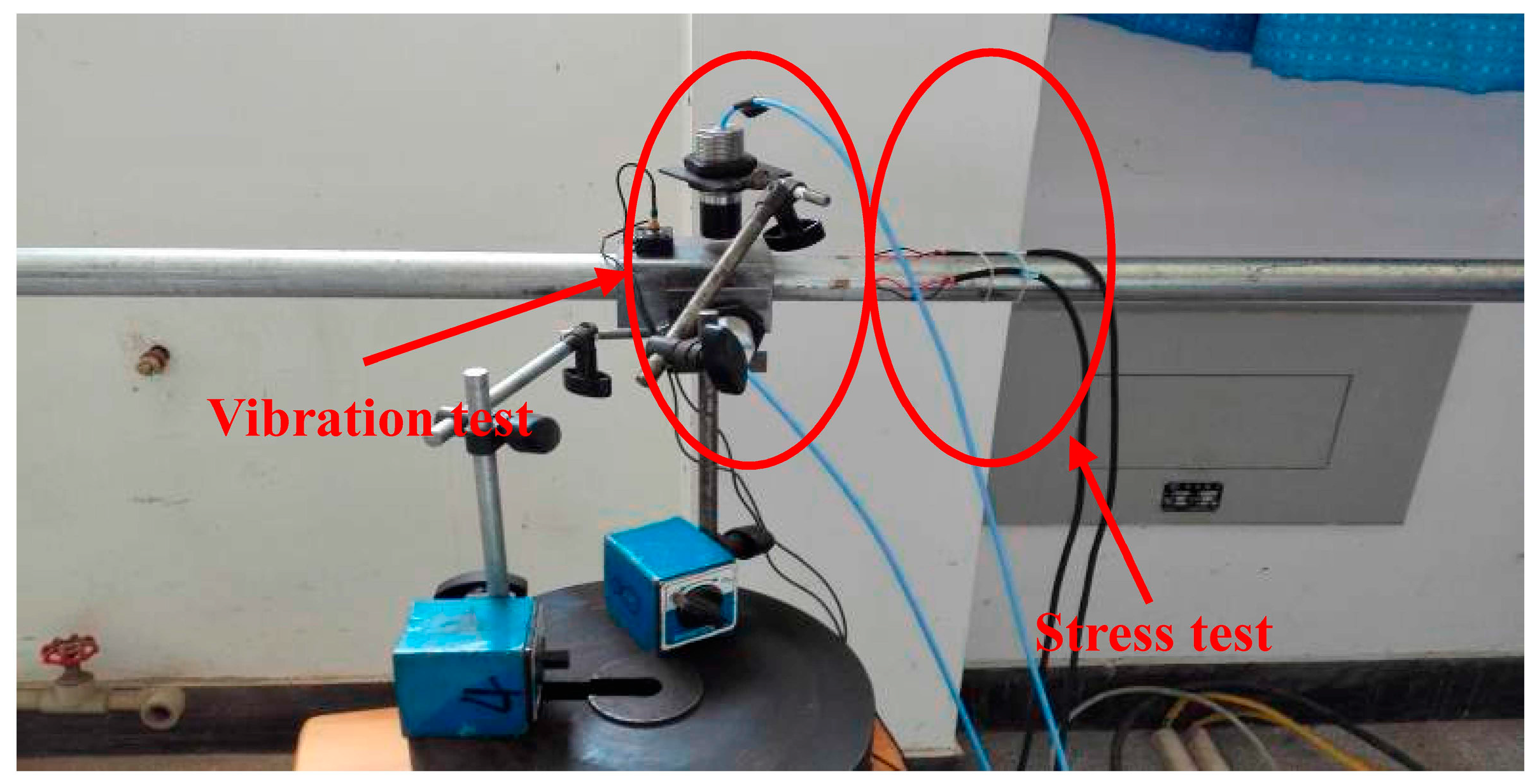
A flat steel plate (size of 40 mm × 40 mm × 1 mm) was mounted on the upper side of the pipe. Acceleration and displacement of the elbow can be obtained from measuring the steel plate’s acceleration and displacement using the piezoelectric three-way acceleration sensor (measuring accuracy is ±1%, frequency response is 1–5 kHz) which is fixed to two test surfaces and the non-contact eddy current displacement sensor (measuring accuracy is ±1%, frequency response is 0–10 kHz) which is parallel to the two test surfaces.

The output flow of piston pump has an obvious regular pulsation, so in order to avoid the non-real-time synchronization acquisition of the data, the TST5912 (Test Electron, Jingjiang, China) dynamic signal test and analysis system and the TST3826F (Test Electron, Jingjiang, China) dynamic and static strain test system were used to simulate the acceleration, displacement, stress and strain of different measuring points. The piston metering pump in supplying a pulsating flow will produce a certain degree of fluctuation due to pressure and flow changes. In the meantime, there will be varying degrees of air in the test pipe section, which will also affect the experimental results. Therefore, in each case, when the working condition is stable, continuous data collection is carried out for a certain period of time, and the data collected in each working cycle are compared and screened to ensure that the data is true and effective.

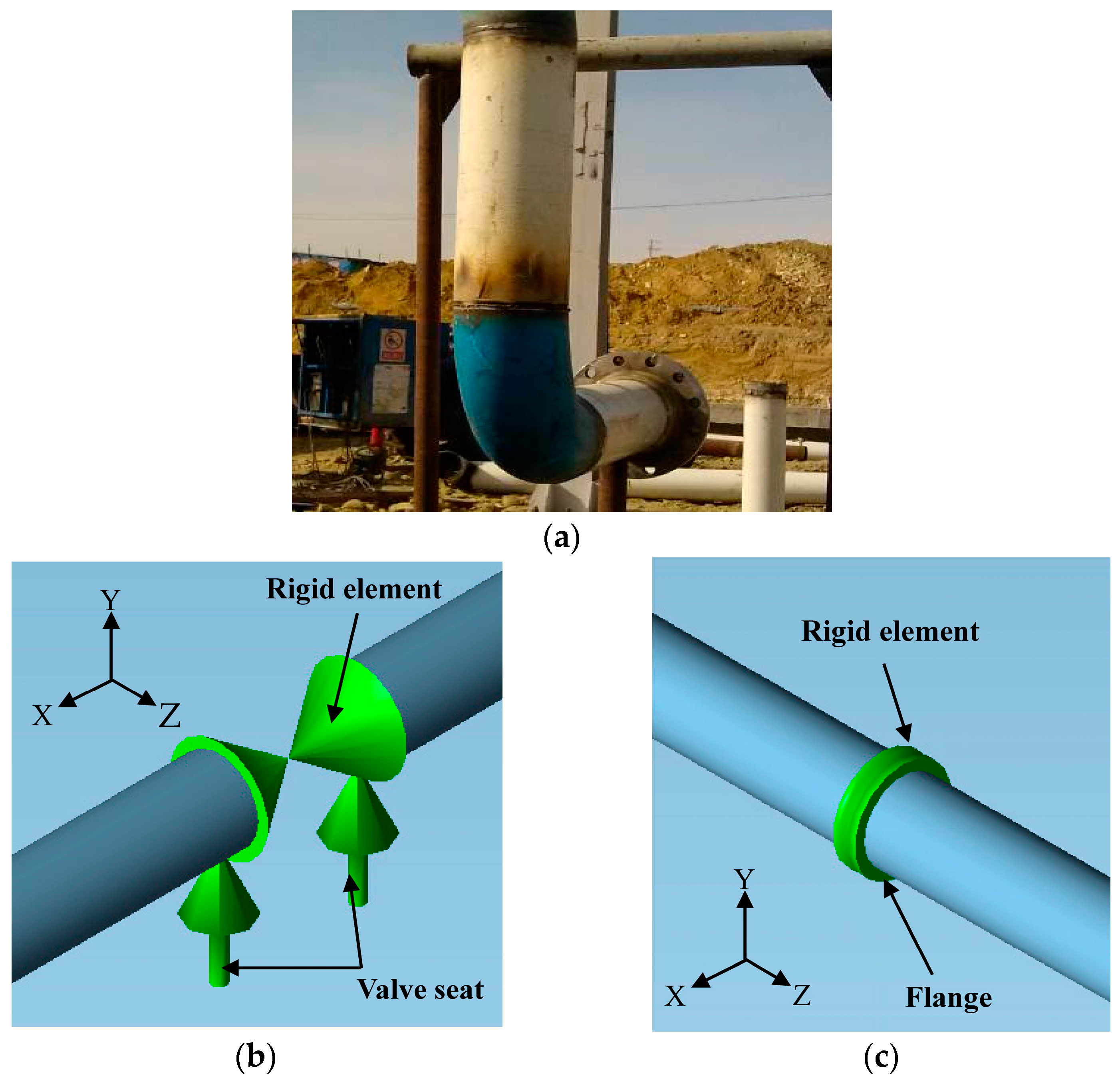
The test pipe is equipped with acceleration sensors, and there are six measuring points. The measuring points 1, 2, 3, 4 and 5 (denoted as TS1, TS2, TS3, TS4 and TS5) are on the straight pipe, and the measuring point 3 is the middle measuring point on the straight pipe. The clamped supported constraints of the straight pipe section and elbow section (taking the 60 degree elbow for instance) can be seen in Figure 8. As shown in Figure 9, the test straight pipe section is 4 m, and a measuring point is added every 1 m. There is only one measuring point at the bend, as shown in Figure 10.

The experimental conditions are listed in

Table 2. Experiment conditions.

Maximum Outlet Pressure P (MPa; ±5%)	Elbow Angle (Degree)	Average Flow Rate Q (L/h; ±2%)
0.9	45	1080	1283
	60	1080	1283
	90	1080	1283
1.2	45	1080	1283
	60	1080	1283
	90	1080	1283
1.4	45	1080	1283
	60	1080	1283
	90	1080	1283

. Before the experiments, the acceleration, displacement sensors, flowmeter and pressure sensors should be corrected. The straight pipe measuring points are marked and the strain gauges stuck on (they are small and light, and will not affect the actual movement of the pipe). Before starting the pump test, we adjust the flow and pressure corresponding to each condition (flow control through the flow meter, control valve to achieve the required pressure value).

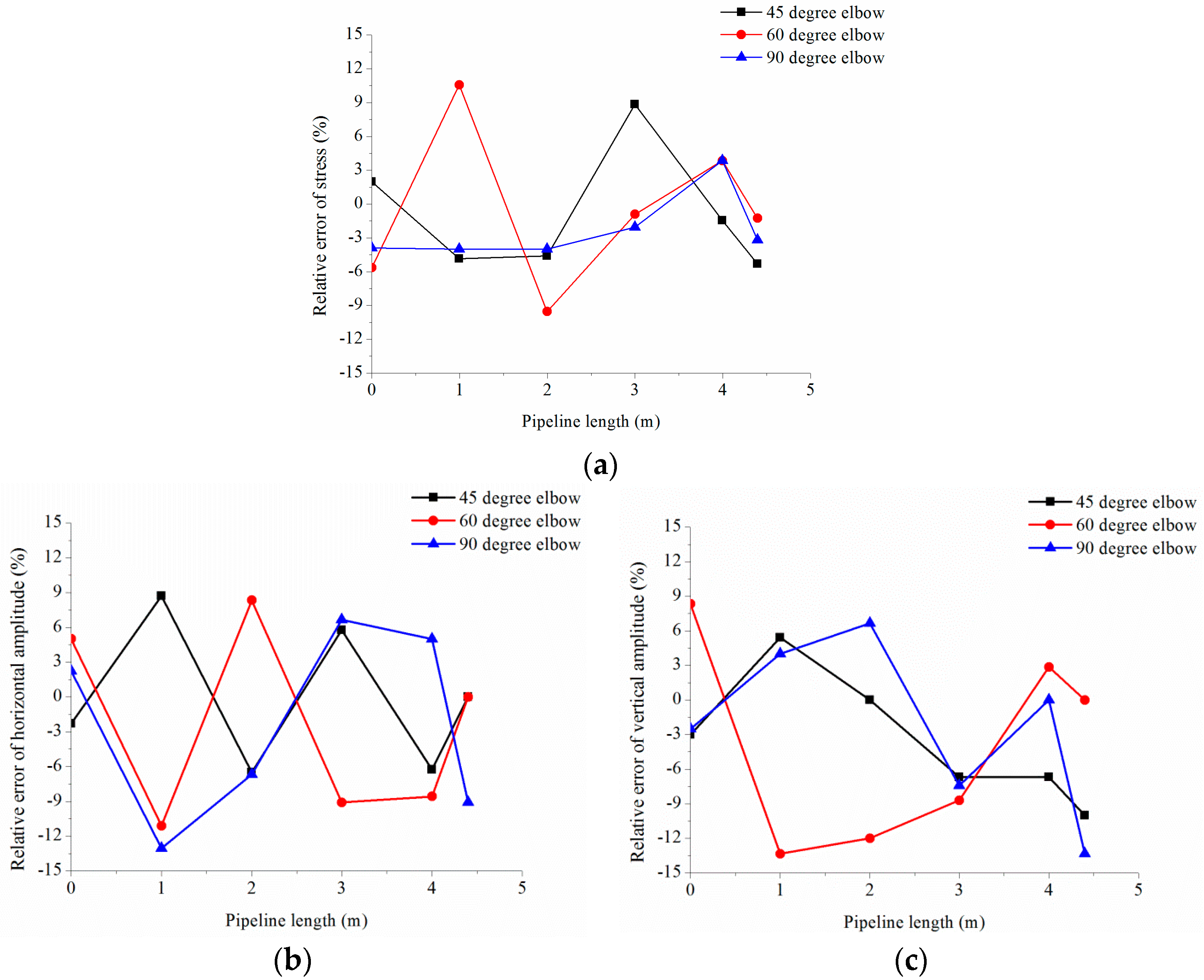
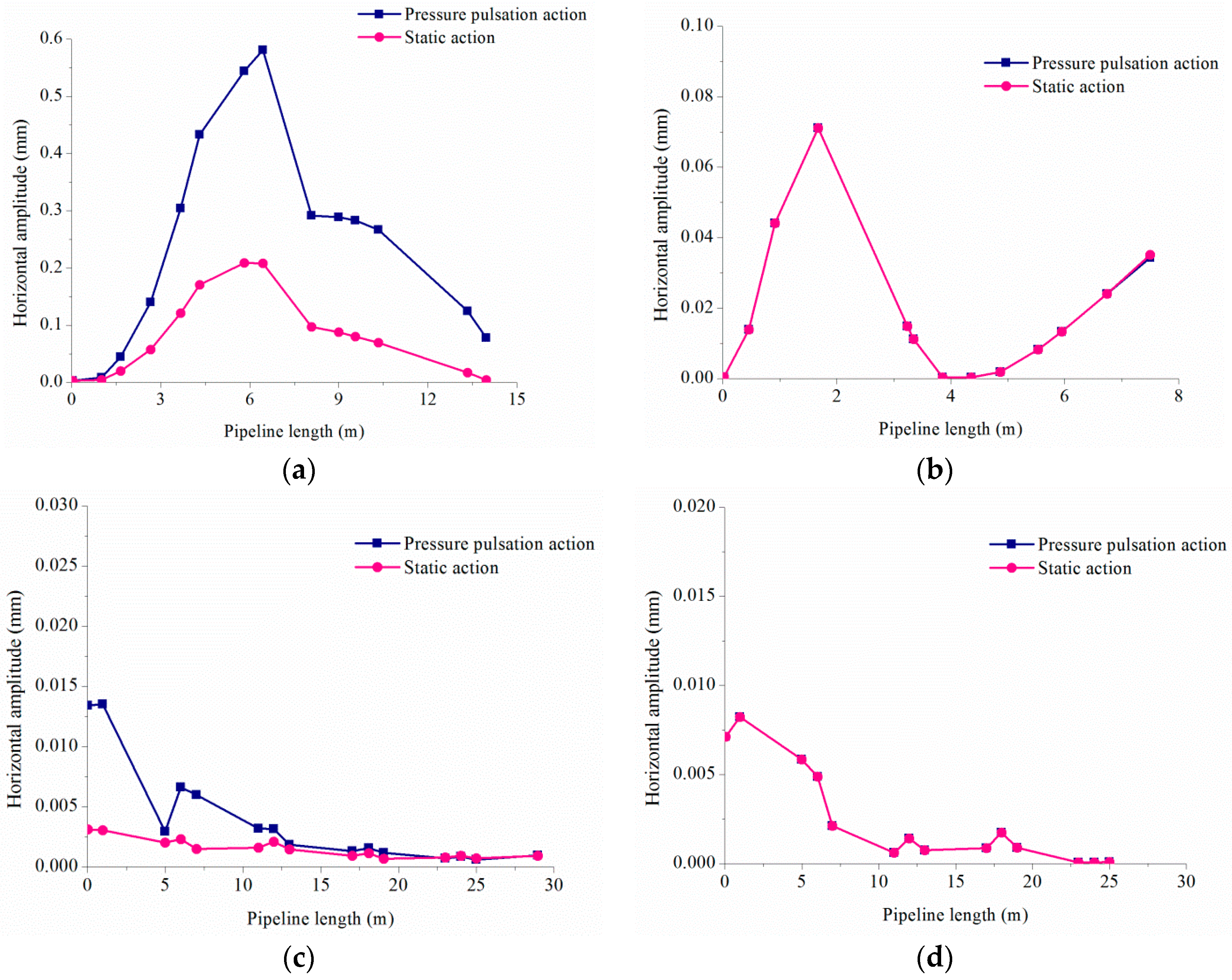
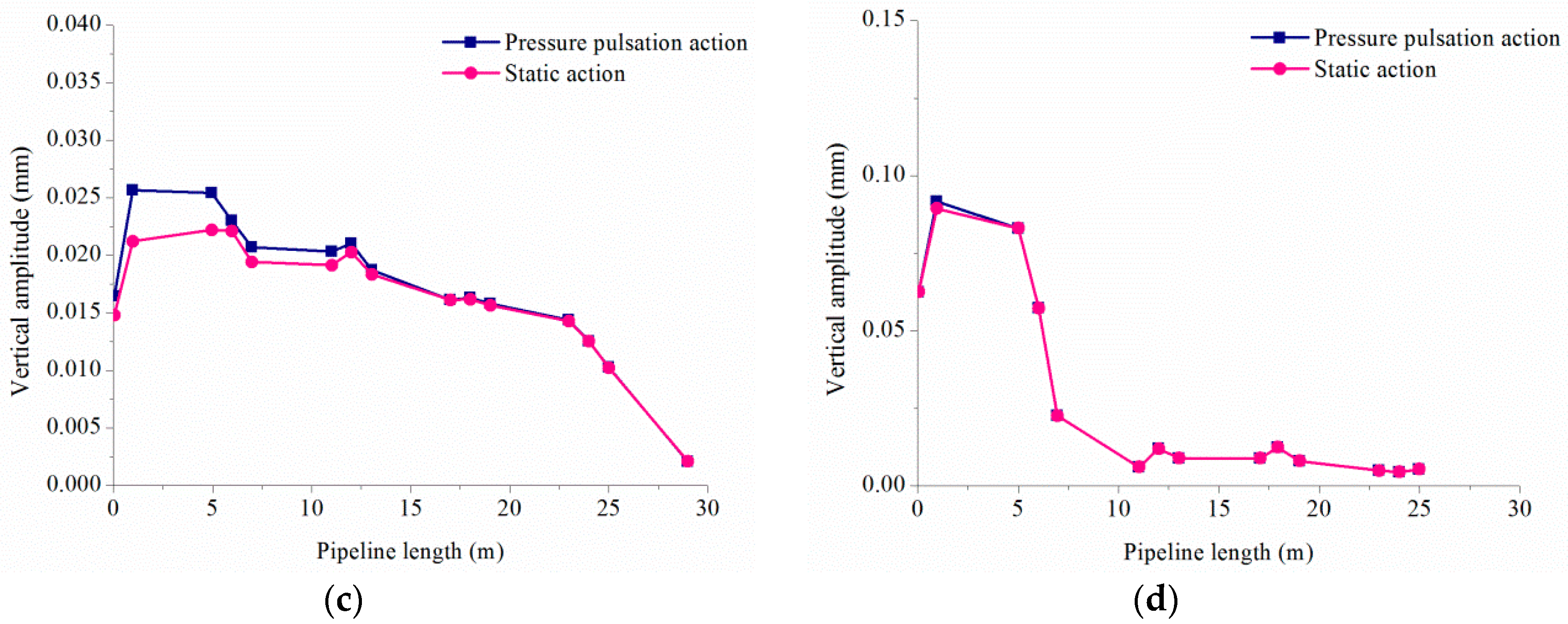
The stress, horizontal and vertical amplitudes test results of the pipeline are shown in Figure 11. The relative error of the experimental and numerical simulation results are shown in Figure 12. From Figure 12, it can be concluded that the relative error range of stress is −9.55–10.57%, the relative error range of horizontal amplitude is −13.04–8.70%, and the relative error range of vertical amplitude is −13.33–8.33%. According to Figure 12, an average relative error can be calculated, as shown in

Table 3. Calculation results of average relative error.

Elbow Angle (Degree)	45	60	90
Stress	4.50%	5.31%	3.50%
Horizontal amplitude	4.93%	7.03%	7.13%
Vertical amplitude	5.31%	7.55%	5.68%

. Based on the above results, the relative error is within the acceptable range (In engineering, the acceptable range refers to the average relative error of numerical simulation and experimental results within 15% [21]), indicating that the numerical simulation method is more feasible.

4. Case Study

4.1. Project Overview

In this paper, the Fengcheng (Xinjiang Uygur Autonomous Region, China) oil station is used as an example of practical application. The station mainly includes pigging area, storage area and transmission area. As the reciprocating pump is located in the transmission area, the pipelines in the transmission area are the object of the study.

The transmission area mainly includes three kinds of equipment: reciprocating pump (piston pump), centrifugal pump and filter. Moreover, this area includes five kinds of pipelines: main inlet pipe, main outlet pipe, sewage pipe, pump inlet pipe and pump outlet pipe. The density of crude oil is 900 kg/m³, and the coefficient of elasticity of the oil at the transportation temperature is 2190 MPa. The distribution of the pipelines is shown in Figure 13, in which the sewage pipe, the main inlet pipe and the main outlet pipe are all buried. The specific pipe parameters are shown in

Table 4. Parameters of the pipelines in the transmission area.

Items	Main Inlet Pipe	Main Outlet Pipe	Sewage Pipe	Pump Outlet Pipe (Reciprocating Pump)	Pump Inlet Pipe (Reciprocating Pump)
Diameter (mm)	355.6	559	89	273	323
Thickness (mm)	9.5	5.2	4	7.8	5.2
Insulation thickness (mm)	60	60	-	60	60
Pipe material	X65	X65	20# steel	X65	X65
Medium density in pipe (kg·m−3)	900	900	-	900	900
Regional level	Level 2
Pipe installation temperature (°C)	10	10	10	10	10
Operating temperature (°C)	95	95	-	95	95
Operating pressure (MPa)	1.6	8	-	8	1.6

, and the soil parameters are shown in

Table 5. Soil parameters.

Soil Properties	Clay
Soil density (kg/m3)	2000
Soil friction angle (Degree)	22
Cohesion (kPa)	50
Overburden compaction multiplier	3
Buried depth (m)	1–2.5

.

Before the vibration analysis of the pipelines in the transmission area, the cause of the vibration should be clarified first. One is directly caused by the pump, the other is the vibration caused by the pressure pulsation. Through field investigation, it is determined that the pump foundation is rammed with reinforced concrete, the rigidity is large, and the pump foundation is connected with the pump body firmly. After examination, no abnormal phenomena such as loosening of anchor bolts was found. According to a vibration instrument and manual inspection, the pump runs smoothly and the vibration is very small. It is clear that the vibration caused by the pump (motor) is not the cause of pipe vibration, and it is clear that the object of this paper is the vibration caused by pipe pressure pulsations.

4.2. Constraint Models of Pipeline

According to the field investigation, the pipeline constraints mainly include: pump nozzle, valve, flange, valve seat, soil.

(1) Pump nozzle

The nozzle and the equipment are connected by flanges. Usually the pump flange is used as a fixed point analog (anchor), which means that the line displacement and angular displacement in the three directions are all bound, and the constraint can be applied to the nozzle without displacement as shown in Figure 14.

(2) Valve and flange

Due to the large rigidity of the valves and flanges on the pipes, it is generally considered that they do not deform in the mechanical analysis and are often represent a concentrated mass, so the model can be simplified by rigid elements, as shown in Figure 15. According to the type of valve and flange, we can find the corresponding weight in the corresponding standard or sample, and enter the data in the model. If its stiffness and mass can not be determined, the stiffness can be taken in accordance with the 10 times the thickness of the nozzle, concentrated quality can be taken in accordance with 1.75 times “weight + medium weight + insulation layer weight”.

(3) Valve seat

The valve seat is equivalent to the load bearing bracket, which is a rigid, one point on the lower part of the pipe, only used to block the downward displacement of the pipe. In CAESAR II, the +Y is represented as a unidirectional upward constraint, indicating that the binding force acts in the +Y direction of the pipe. As the pipe moves relative to the structure, a friction model must be established, in which the direction of the friction force is the same as the direction of the pipe movement, as shown in Figure 15b. The coefficient of friction is defined between the valve seat and the valve, for the contact between steel and steel, the coefficient of friction is 0.3.

(4) Four-directional guide

A four-directional guide is usually used in the oil station to limit the displacement of the pipe in the horizontal and vertical directions. It has a good effect on the control vibration. Like the one-way constraint, the friction coefficient is defined when the constraint is set, as shown in Figure 16.

(5) Soil

The ALA (American Lifelines Alliance) model was used in soil section, and a practical description can be found in [5].

4.3. Pipeline Overall Model

The overall model of FC oil station can be seen in Figure 17, and a partial magnification can be seen in Figure 18.

4.4. Action Location and Calculation Result of Unbalanced Exciting Force

The calculation results of the unbalanced exciting force of the RP1 pump outlet pipe and the pump inlet pipe at the elbow and tee are shown in

Table 6. Calculation results of unbalanced exciting force of RP1 pump pipe.

Pipe Type	Location	Pressure Pulsation ΔP (Pa)	Unbalanced Exciting Force (N)	Direction	Phase Angle (Degree)
Pump outlet pipe	RP1-B1	14,885.64	1094.09	Y	0
	RP1-B2	43,780.53	−3217.87	Z	3.05
	RP1-B3	67,202.83	−4939.41	Y	5.52
	RP1-B4	146,123.10	−10,740.05	X	14.21
Main outlet pipe	T1	184,644.40	−13,571.36	Y	18.64
Pump inlet pipe	RP1-B5	2874.95	310.49	Z	0
	RP1-B6	15,768.83	−1703.03	X	6.72
Main inlet pipe	T2	23,691.54	−2558.69	Y	11.29

. The location of the unbalanced exciting force is shown in Figure 19.

5. Results

In order to study the influence of pressure pulsation on the pipeline, this paper analyzes two working conditions: (1) RP1 pump runs separately; (2) RP1 and RP2 run together.

5.1. RP1 Pump Runs Separately

Figure 20 and Figure 21 show the maximum amplitudes of the horizontal and vertical directions of each pipe, and

Table 7. Summary of the maximum amplitude and location.

Pipeline Type	Horizontal Direction		Vertical Direction
	Amplitude (mm)	Location	Amplitude (mm)	Location
RP1 pump outlet pipe	0.58	RP1-B3	0.14	RP1-B4
RP1 pump inlet pipe	0.07	RP1-B5	0.06	RP1-B6
Main outlet pipe	0.01	T1	0.03	Middle of T1 and T3
Main inlet pipe	0.008	T2	0.09	T2

shows the summary of the maximum amplitude and location.

It can be concluded from Table 7 that the maximum horizontal or vertical amplitude of each pipe are mostly produced in the elbow and tee, and the horizontal amplitude of the elbow is larger than the vertical amplitude. However, the vertical amplitude is greater than the horizontal amplitude at the tee of the straight pipe section. In addition, the following conclusions can be obtained:

(1)

The unbalanced exciting force has a great influence on the vibration of the pump outlet pipe (the amplitude increases by 5–140%) and the main outlet pipe (the amplitude increases by 5–360%), and has little influence on the vibration of the pump inlet pipe (the amplitude increases by 1–10%).

(2)

Although the unbalanced exciting force is generated at the elbow, the vibration of the straight pipe is affected to varying degrees (it rises).

5.2. RP1 and RP2 Run Together

Table 8. Summary of the maximum amplitude and location.

Pipeline Type	Horizontal Direction		Vertical Direction
	Amplitude (mm)	Location	Amplitude (mm)	Location
RP1 pump outlet pipe	0.40	RP1-B3	0.12	RP1-B4
RP1 pump inlet pipe	0.07	RP1-B5	0.06	RP1-B6
RP2 pump outlet pipe	0.67	RP2-B3	0.15	RP2-B4
RP2 pump inlet pipe	0.07	RP2-B5	0.06	RP2-B6
Main outlet pipe	0.01	T3	0.03	T3
Main inlet pipe	0.01	T2	0.09	T2

shows the summary of the maximum amplitude and location.

According to Table 7 and Table 8, the situations of single pump operation and double pumps operation are compared, and the main conclusions are as follows:

(1)

In the case of double pump operation, the maximum horizontal amplitude and vertical amplitude of the RP1 pump outlet pipe are significantly lower than those of the case of RP1 single pump operation (the horizontal amplitude decreases by about 31%, and the vertical amplitude decreases by about 15%), the change of horizontal amplitude and vertical amplitude of the RP1 pump inlet pipe is not obvious, and the amplitude of RP2 pump outlet pipe is higher than that of RP1 pump in all directions.

(2)

Whether the single pump operation or multi pump operation, the pump outlet pipe has the largest amplitude, so the emphasis of the vibration reduction study is outlet pipe of the pump.

6. Discussions

In this paper, several factors influencing the vibration of the pipeline are analyzed: flow, pressure, temperature, crude oil density and foundation settlement, and the measures of vibration reduction are put forward.

6.1. Flow Rate

A flow fluctuation will occur during the reciprocating pump operation, according to the testing data of the FC oil station, when the flow rate of single pump is 220 m³/h, and the minimum flow rate is 71.4% of the normal pump output, that is, 157.08 m³/h. Therefore, this paper takes the RP1 pump outlet pipe for instance, the vibrations of pipe in the case of flow rate from 150 m³/h to 220 m³/h are discussed. The results can be seen in

Table 9. The maximum amplitudes of RP1 outlet pipe at different flow rates.

Flow Rate (m3/h)	Horizontal Vibration		Vertical Vibration
	Amplitude (mm)	Location	Amplitude (mm)	Location
150	0.572	RP1-B3	0.136	RP1-B4
160	0.573		0.136
170	0.573		0.136
180	0.575		0.137
190	0.576		0.138
200	0.577		0.139
210	0.579		0.139
220	0.580		0.140

.

It can be concluded from Table 9 that: the flow rate change of the reciprocating pump has little effect on the amplitude of the pipe vibration.

6.2. Pressure

The actual operation pressure of the pipeline is lower than the design pressure, and the regulation of pressure is frequency conversion control. For the FC oil station, when the pump outlet manifold pressure is higher than 7.04 MPa, the reflux valve opens; when the pump outlet manifold pressure is higher than 8 MPa, the oil pump automatically stops. Therefore, the vibrations of pipe in the case of pressure from 6.0 MPa to 8.0 MPa are discussed. The results can be seen in

Table 10. The maximum amplitudes of RP1 outlet pipe at different pressures.

Pressure (MPa)	Horizontal Vibration		Vertical Vibration
	Amplitude (mm)	Location	Amplitude (mm)	Location
6.0	0.517	RP1-B3	0.127	RP1-B4
6.5	0.527		0.130
7.0	0.535		0.135
7.5	0.575		0.137
8.0	0.580		0.140

. From Table 9, it can be concluded that the horizontal amplitude and vertical amplitude increase with the increase of pressure.

6.3. Temperature

Because FC oil station transports heavy oil, the oil temperature is higher (up to 95 °C), so in order to explore the influence of temperature on the pipeline vibration, the vibrations of pipe in the case of temperature from 25 °C to 95 °C are discussed. The results can be seen in Figure 22.

As shown in Figure 22, with the increase of temperature, the horizontal amplitude of pipeline (95 °C and 10 °C compared) increased by about 64%, the vertical amplitude increased by 2729%, and when the temperature is higher than 85 °C, the influence of temperature on the vertical amplitude has improved significantly.

6.4. Crude Oil Density

According to the design data, the crude oil density of FC oil station is in the range of 850–950 kg/m³, and the influence of crude oil density on pipeline vibration is discussed.

As shown in

Table 11. Maximum amplitudes of RP1 outlet pipe at different crude oil densities.

Crude Oil Density (kg/m3)	Horizontal Vibration		Vertical Vibration
	Amplitude (mm)	Location	Amplitude (mm)	Location
850	0.577	RP1-B3	0.139	RP1-B4
900	0.580		0.140
950	0.585		0.143

, the maximum horizontal amplitude and vertical amplitude increase with the increase of crude oil density, but the change is little, which shows that the density of crude oil has little influence on the vibration of reciprocating pump pipes.

6.5. Foundation Settlement

Many pipelines are laid on soft soils. The foundation has a low bearing capacity and a large deformation after loading. It is easy for the pipeline to crack, and become twisted or inclined due to foundation settlement. In this paper, the foundation settlement of the pump outlet pipe is discussed. There are two possible locations for foundation settlement: fulcrum 1 and fulcrum 2.

This paper discusses the pump outlet pipe to produce fulcrum foundation settlement situation, there may be two places of settlement: fulcrum 1 and fulcrum 2 (as shown in Figure 23), are the valve seat on the pipeline. The operation conditions of foundation settlement can be seen in

Table 12. Operation conditions of foundation settlement.

Operation Conditions	Description
1	Fulcrum 1 settlement
2	Fulcrum 1 and the fulcrum 2 all have settlement
3	Fulcrum 2 settlement
4	Fulcrum 1 and the fulcrum 2 are free of settlement

, and the settlement is assumed to be 3 cm.

It can be seen from Figure 24, the amplitude of the condition 2 is the maximum in the four conditions, and the increase is obvious. The amplitude of the condition 1 is larger than that of the condition 3, indicating that the settlement of the fulcrum 1 is more dangerous in the case of a single fulcrum settlement. In actual engineering, the fulcrum 1 and fulcrum 2 should be prevented from settling at the same time.

6.6. Vibration Reduction Measures

In engineering, vibration reduction can be achieved by increasing the rigidity of the pipeline. The greater the rigidity, the higher the natural frequency of the pipe, the less likely it is to cause resonance. Usually, four-directional guide are added in the vicinity of the elbow. Therefore, considering the eight locations of constraints added to the pump outlet pipe, as shown in Figure 25, the natural frequency is calculated. The analysis results are shown in

Table 13. First order natural frequency of the pump outlet pipe after the constraint is added.

Location of the Constraint	First Order Natural Frequency (Hz)
L1	6.97
L2	6.98
L3	6.99
L4	7.00
L5	7.02
L6	7.29
L7	10.76
L8	9.75

.

As can be seen in Table 13, adding the four-directional guide to the L7 position improves the first order natural frequency of the pump outlet pipe preferably, so when the pipeline is modified, the four-directional guide may be added to the L7 position. At the same time, evaluate the amplitude of pipe after L7 after the constraint is added, the maximum amplitude decreased from 0.58 mm to 0.27 mm, the maximum amplitude of the horizontal direction decreased from 0.14 mm to 0.04 mm. Therefore, the addition of four-directional guide at L7 location can effectively reduce the pipeline vibration amplitude. Since there is only one elbow in the vicinity of the L7 location and the constraint is less, it can be deduced: The restraint can be greatly reduced by adding constraints to the long straight pipe with few bends and few constraints.

7. Conclusions

In this paper, the method of vibration analysis of the reciprocating pump pipeline system is put forward by means of numerical simulation and indoor experiments. By analyzing a project example, the vibration law of the pipeline system is obtained, and the corresponding vibration reduction measures are put forward. The main conclusions are as follows:

(1)

The maximum horizontal or vertical amplitude of each pipe is mostly produced in the elbow and tee, and the unbalanced exciting force has a great influence on the vibration of the pump outlet pipe (the rate of increase is up to 140%) and the main outlet pipe (the rate of increase is up to 360%). Although the unbalanced exciting force is generated at the elbow, the vibration of the straight pipe is affected to varying degrees.

(2)

The flow rate change of the reciprocating pump and the density of crude oil have little effect on the amplitude of the pipe. The horizontal amplitude and vertical amplitude increase with the increase of pressure. When the temperature is higher than 85 °C, the influence of temperature on the vertical amplitude has improved significantly.

(3)

In actual engineering, it should be possible to prevent the simultaneous settlement of multiple places.

(4)

The amplitude can be greatly reduced by adding constraints to a long straight pipe with few bends and few constraints.

References

1. Wang, Y. Large property damage losses in the hydrocarbon-chemical industries. Petrol. Plan. Eng. 1993, 4, 59–60. [Google Scholar]
2. Ye, L.H. Research on the Vibration and Damping Strategy of the Outlet Pipeline of Water Injection Pump in Oil Field. Master’s Thesis, Huazhong University of Science and Technology, Wuhan, China, 2009. [Google Scholar]
3. Wachel, J.C.; Szenasi, F.R.; Denison, S.C. Analysis of vibration and failure problems in reciprocating triplex pumps for oil pipelines. In Proceedings of the Energy-Sources and Technology Conference and Exhibition, Dallas, TX, USA, 17–21 February 1985. [Google Scholar]
4. Chen, H.H. Vibration Damping Analysis and Optimization Design of the Reciprocating Compressor Pipeline. Master’s Thesis, Beijing University of Chemical Technology, Beijing, China, 2014. [Google Scholar]
5. Lu, H.F. Stress and Vibration Analysis of Reciprocating Pump Piping Systems. Master’s Thesis, Southwest Petroleum University, Chengdu, China, 2016. [Google Scholar]
6. Chen, H.F. Research of Piping Vibration Characteristics of Reciprocating Compressor and Safety Assessment. Master’s Thesis, China University of Petroleum (East China), Qingdao, China, 2009. [Google Scholar]
7. Bickford, W.B.; Strom, B.T. Vibration of plane curved beams. J. Sound Vib. 1975, 39, 135–146. [Google Scholar] [CrossRef]
8. Paidoussis, M.P.; Laithier, B.E. Dynamics of Timoshenko beams conveying fluid. J. Mech. Eng. Sci. 1976, 18, 210–220. [Google Scholar] [CrossRef]
9. Irie, T.; Yamada, G.; Takahashi, I. Vibration and stability of a non-uniform Timoshenko beam subjected to a follower force. J. Sound Vib. 1980, 70, 503–512. [Google Scholar] [CrossRef]
10. Lesmez, M.W.; Wiggert, D.C.; Hatfield, F.J. Modal analysis of vibrations in liquid-filled piping systems. J. Fluid Eng. 1990, 112, 311–318. [Google Scholar] [CrossRef]
11. Ashley, H.; Haviland, G. Bending vibrations of a pipe line containing flowing fluid. J. Appl. Mech. 1950, 17, 229–232. [Google Scholar]
12. Fuller, C.R.; Fahy, F.J. Characteristics of wave propagation and energy distributions in cylindrical elastic shells filled with fluid. J. Sound Vib. 1982, 81, 501–518. [Google Scholar] [CrossRef]
13. Adachi, T.; Ujihashi, S.; Matsumoto, H. Impulsive responses of a circular cylindrical shell subjected to waterhammer waves. J. Press. Vessel Technol. 1991, 113, 517–523. [Google Scholar] [CrossRef]
14. Yu, C.L.; Wei, Y.; Hu, X.M. Piping vibration analysis for the type of reciprocating compressor. China Offshore Platf. 2007, 22, 52–56. [Google Scholar]
15. Zhou, H.; Liu, Y.S.; Yue, Z.F. Calculation analyze of pressure pulsation in fluid flowing pipeline. Mech. Sci. Technol. Aerosp. Eng. 2011, 30, 1435–1438. [Google Scholar]
16. Lu, H.F.; Huang, K.; Wu, S.J. Vibration and stress analyses of positive displacement pump pipeline systems in oil transportation stations. J. Pipeline Syst. Eng. 2016, 7, 05015002. [Google Scholar] [CrossRef]
17. Bruggeman, J.C. Flow Induced Pulsations in Pipe Systems. Ph.D. Thesis, Technische Universiteit Eindhoven, Eindhoven, The Netherlands, 1987. [Google Scholar]
18. Frosina, E.; Senatore, A.; Rigosi, M. Study of a high-pressure external gear pump with a computational fluid dynamic modeling approach. Energies 2017, 10, 1113. [Google Scholar] [CrossRef]
19. Vasilyev, P.; Fromzel, L. Analytical Study of Piping Flow-Induced Vibration, Example of implementation. In Proceedings of the 17th International Conference on Structural Mechanics in Reactor Technology, Prague, Czech Republic, 17–22 August 2003. [Google Scholar]
20. Siba, M.; Wanmahmood, W.; Nuawi, M.Z.; Rasani, R.; Nassir, M. Flow-induced vibration in pipes: Challenges and solutions—A review. J. Eng. Sci. Technol. 2016, 11, 362–382. [Google Scholar]
21. Zhou, X.P.; Peng, X.Q.; Zhang, S. Numerical simulation of wind pressures on the gable roof with cantilevered parapets. J. Huaqiao Univ. (Nat. Sci.) 2008, 29, 289–293. [Google Scholar]
Figure 1. Vibration analysis process of a reciprocating pump pipeline.
Energies 11 00132 g001
Figure 2. Elbow force diagram.
Energies 11 00132 g002
Figure 3. Schematic diagram of a simple pipe model.
Energies 11 00132 g003
Figure 4. Pipeline foundation model and constraint model of the simple pipe established by CAESAR II software: (a) overall model; (b) constraints’ model.
Energies 11 00132 g004
Figure 5. Pressure pulsation at the first 100 s of the elbow.
Energies 11 00132 g005
Figure 6. Horizontal and vertical amplitudes of pipelines with different elbow degrees: (a) stress; (b) horizontal amplitude; (c) vertical amplitude.
Energies 11 00132 g006
Figure 7. Schematic diagram of experiment.
Energies 11 00132 g007
Figure 8. Physical map of clamped supported constraints: (a) straight pipe section; (b) elbow pipe section.
Energies 11 00132 g008
Figure 9. Physical map of pipe vibration test device and stress test device in straight pipe section.
Energies 11 00132 g009
Figure 10. Physical map of pipe vibration test device and stress test device in elbow section.
Energies 11 00132 g010
Figure 11. Test results of pipeline: (a) stress; (b) horizontal amplitude; (c) vertical amplitude.
Energies 11 00132 g011
Figure 12. Relative error of the experimental and numerical simulation results: (a) stress; (b) horizontal amplitude; (c) vertical amplitude.
Energies 11 00132 g012
Figure 13. Sketch map of pipeline distribution in the transmission area (Note: RP represents the reciprocating pump, CP represents centrifugal pump).
Energies 11 00132 g013
Figure 14. Pump nozzle: (a) physical map and (b) numerical simulation model in CAESAR II software.
Energies 11 00132 g014
Figure 15. Rigid element: (a) physical map of flange; (b) numerical simulation model of valve in CAESAR II software; (c) numerical simulation model of flange in CAESAR II software.
Energies 11 00132 g015
Figure 16. Numerical simulation model of four-directional guide in CAESAR II software.
Energies 11 00132 g016
Figure 17. Overall model of the pipelines and equipment of the transmission area.
Energies 11 00132 g017
Figure 18. Partial magnification model.
Energies 11 00132 g018
Figure 19. The location of the unbalanced exciting force.
Energies 11 00132 g019
Figure 20. Horizontal amplitude of pipes: (a) RP1 pump outlet pipe; (b) RP1 pump inlet pipe; (c) main outlet pipe; (d) main inlet pipe.
Energies 11 00132 g020
Figure 21. Vertical amplitude of pipes: (a) RP1 pump outlet pipe; (b) RP1 pump inlet pipe; (c) main outlet pipe; (d) main inlet pipe.
Energies 11 00132 g021aEnergies 11 00132 g021b
Figure 22. Amplitude distribution of RP1 pump outlet pipe at different temperatures: (a) horizontal amplitude; (b) vertical amplitude.
Energies 11 00132 g022
Figure 23. Foundation settlement locations.
Energies 11 00132 g023
Figure 24. Horizontal and vertical amplitudes of four settlement conditions.
Energies 11 00132 g024
Figure 25. Eight locations of constraints added to the pump outlet pipe.
Energies 11 00132 g025