Article

Application of Predictive Feedforward Compensator to Microalgae Production in a Raceway Reactor: A Simulation Study

1
Departamento de Informática y Automática, ETSII, UNED, 28040 Madrid, Spain
2
Departamento de Informática, University of Almería, CIESOL-ceiA3, 04120 Almería, Spain
3
Departamento de Ingeniería, University of Almería, CIESOL-ceiA3, 04120 Almería, Spain
*
Author to whom correspondence should be addressed.
Energies 2018, 11(1), 123; https://doi.org/10.3390/en11010123
Submission received: 24 November 2017 / Revised: 22 December 2017 / Accepted: 2 January 2018 / Published: 4 January 2018

Abstract

:
In this work, the evaluation of a predictive feedforward compensator is provided in order to highlight its most important advantages and drawbacks. The analyzed technique has been applied to microalgae production process in a raceway photobioreactor. The evaluation of the analyzed disturbance rejection schemes were performed through simulation, considering a nonlinear process model, whereas all controllers were designed using linear model approximations resulting in a realistic evaluation scenario. The predictive feedforward disturbance compensator was coupled with two feedback control techniques, PID (Proportional-Integral-Derivative) and MPC (Model Predictive Control) that are widely used in industrial practice. Moreover, the classical feedforward approach has been used for the purpose of comparison. The performance of the tested technique is evaluated with different indexes that include control performance measurements as well as biomass production performance. The application of the analyzed compensator to microalgae production process allows us to improve the average photosynthesis rate about 6% simultaneously reducing the energy usage about 4%.

1. Introduction

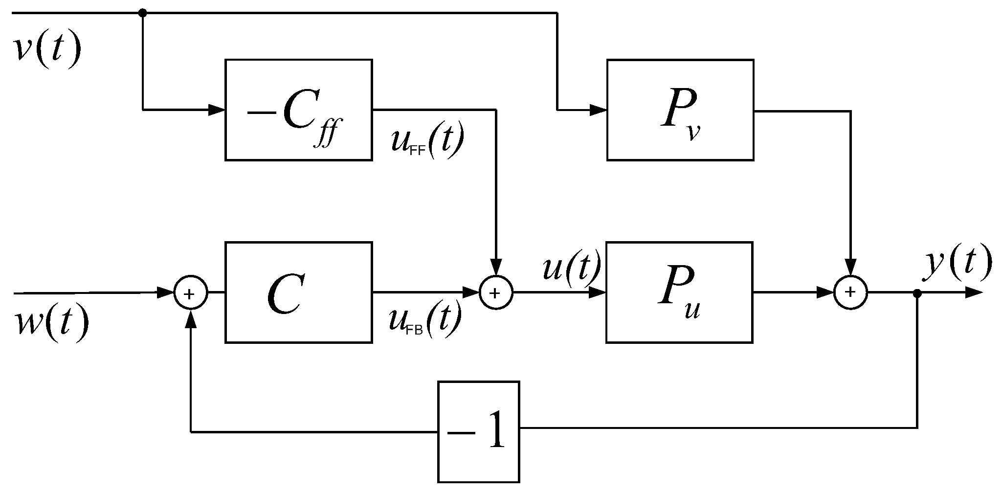
Disturbance compensation is a very important aspect that needs to be considered in control system design for a particular process [1]. In such a case, the control technique should be able to maintain the controlled variable close to the reference despite the external disturbances that influence the controlled process. For this reason, most industrial processes need a personalized control scheme to achieve the performance requirements [2]. From a control system point of view, the process disturbances can be grouped as unmeasurable and measurable quantities depending on their origin. The measurable disturbances can be handled by the feedforward structure that can compensate the disturbance before its effect appears on the controlled variable. However, in many industrial applications, the control system consists of a feedback controller, since it is able to provide a set point tracking, reduces the influence of plant-model mismatch as well as compensates for process disturbances [1,3]. Due to this simple structure, the control system focuses only on one of these issues and provides weak performance for the other problems [4]. In the classical approach, the feedforward compensator is obtained as the quotient between the disturbance and the process dynamics. Nevertheless, this structure is rarely realizable, e.g., due to dead time inversion issues. This problem has been analyzed by several researchers during the past decades and drives to design more advanced tuning rules for feedforward schema [5]. Other approach to measurable disturbance compensation consists in the application of the MPC (Model Predictive Control) technique. Due to simultaneous solution for feedback as well as feedforward control, this control technique is frequently used in industrial processes [6,7]. Regarding the feedforward action, the most relevant advantage of the MPC algorithm is related to the prediction mechanism that can handle future disturbance information [8,9]. Nevertheless, considering the internal relationship, the MPC feedforward and feedback co-design needs a compromise, where the design is oriented considering the most relevant aspects [10,11].
Taking into account all these properties, a new predictive feedforward compensator has been recently proposed in [12], merging advantages of classical MPC-based solutions. In this case, the compensator can be easily coupled with any feedback controller and its design is independent of other elements in the control loop. Moreover, it is also able to consider future disturbance estimations to improve a disturbance attenuation.
The disturbance compensation aspects are also very important in bio-processes, where the control technique has to reduce the influence of external disturbances [13,14], and this is the case of microalgae production in raceway reactors. In such a system, the main task of the controller is to compensate for the influence of external disturbances that affect the photosynthesis rate. The microalgae culture is influenced by many factors, where the most important variables are related to: solar light viability, temperature of the medium, dissolved oxygen and medium pH [15]. In this context, a proper disturbance attenuation could improve the control system accuracy and, as a consequence, the biomass production performance. The remaining variables of the microalgae cultivation process such as dissolved oxygen and pH need to be regulated using a proper control system [16]. Both variables, dissolved oxygen and pH, are characterized by highly changing dynamics (influenced by solar radiation and photosynthesis rate) and their values should be maintained within optimal values for each strain. The photosynthesis rate is influenced mostly by solar irradiance, temperature and pH among others. It is well known that injection of CO2 has a strong influence on the pH level since it affects the growth medium. Moreover, the usage of CO2 represents important operational expense for microalgae culture and its supply excess should be avoided [17]. Taking advantage of this relationship, the control approach uses the pH value to define the amount of CO2 and time instance for its injection [18,19]. Considering all previously mentioned aspects, the disturbance compensation scheme can play a decisive role in boosting control performance and improving the rentability in biomass production process.
In this study, we provide a practical evaluation of a predictive disturbance compensation technique introduced in [12] in order to highlight the most important advantages and drawbacks of such a scheme. As was shown in previous works [12,20], the main advantage of such a technique is the ability to handle the complex dynamics required for perfect disturbance compensation. In the analysis performed previously, a complete knowledge of the process model was assumed and the future disturbance signal was known a priori [20]. From the theoretical point of view, these assumptions allow us demonstrate that predictive feedforward compensator is able to compensate completely the disturbance before its effect appears on the controlled variable. Nevertheless, this assumption can be rarely achieved in an industrial control system, where the usage of simplified models is a common practice. Moreover, the future values of disturbance signals need to be estimated, which also introduces additional uncertainty resulting in performance degradation. Additionally, in this work, the original approach based on a GPC (Generalized Predictive Control) algorithm is extended, with a constraints’ handling mechanism in the feedforward controller being a new future and very important aspect from practical implementation point of view. Moreover, state of the future disturbances required for predictive mechanism is estimated using a Double Exponential Smoothing (DES) technique that was proposed in [8] for MPC control techniques where future information on disturbance signal is required. In the performed study, we use PID and MPC techniques as a feedback controllers that are coupled with the predictive feedforward compensator to show its influence on the control performance in two cases. The evaluation is performed on the biomass production process using a raceway photobioreactor model developed in [21]. The test bed is built using a first principle raceway reactor model as a process plant and all controllers are developed using linear model approximations obtained close to its operating point. This approach considers a plant-model mismatch allowing us create a realistic control scenario. Taking into account all these features, it is possible to obtain results similar to those obtained in the real plant. However, the implementation in simulation environments has the advantage of the repeatability of the external parameters that influence the control system. In such a way, the changes in production performance depend only on the applied control techniques and giving measurable changes in biomass production. All the analyzed control systems are evaluated using control performance as well as biomass production indexes. Additionally, the test bed system is evaluated in terms of energy usage efficacy.

2. Feedforward Compensators

This section is devoted to introducing the disturbance compensation approaches used in the performed analysis. First, the classical approach is introduced and combined with a PID controller. Next, the GPC-based implicit feedback/feedforward structure is described. Afterwards, predictive feedforward compensator originally introduced in [12] is summarized. Moreover, the previous approach is extended with constraints handling mechanism and the future disturbance estimation technique is also provided.
It needs to be highlighted that, in this paper, we analyze the disturbance rejection problem in a process that is affected by dead time. This issue makes the classical feedforward compensator less effective and a more complex compensator is required. This is due to dead time inversion issues (see [20] for more details). Moreover, for simplicity, the process, P u , and the disturbance dynamics, P v , are represented by a first order system with dead time using the following representation:
P u ( s ) = K u 1 + s T u e s d u , P v ( s ) = K v 1 + s T v e s d v .

2.1. Classical Feedforward Structure for Disturbance Compensation

The block diagram of a classical feedforward disturbance compensation problem is shown in Figure 1 and consists of a feedback controller C, process P u , a feedforward controller C f f and process P v , which relates a measurable load disturbance v with the process output y. The remaining signals are: set point w, control signal u (composed of u F F and u F B provided by feedforward and feedback controllers). In this scheme, the load disturbance is fed through a feedforward compensator whose output is added to the feedback control action. From the process control point of view, the goal of this structure consists in a feedforward compensator design in a way that the influence of the measurable disturbance on the controlled process is minimized.
Using block algebra, it can be seen that the analytical expression for disturbance compensation is given by:
y v = P v C f f P u 1 + C P u ,
and, from this expression, it can be observed that the disturbance can be completely attenuated when C f f = P v / P u . Nevertheless, the resulting compensator is rarely realizable, since it could contain unstable or non-causal dynamics, and thus other developments should be investigated.
In a first approach, low-order feedforward and feedback controllers are considered. In this case, we consider a PI or PID controller as the feedback controller, such that:
C ( s ) = K 1 + 1 s T i + s T d ,
where K refers to proportional gain, T i is the integral time and T d is the derivative time ( T d = is set to 0 if a PI controller is used). Note that, in a real implementation, features like filters, anti-windup and limitations must be added [1]. In addition, we also assume a low-order feedforward compensator (a lead-lag filter with a dead time), such that:
C f f ( s ) = K f f 1 + s B f f 1 + s T f f e s L f f ,
and K f f , 1 / B f f , 1 / T f f and L f f refers to the static gain the zero, the pole and the dead time, respectively. Note that more complex structures are seldom used [22] in practice.
Taking into account the aforementioned process transfer functions, it is possible to achieve perfect disturbance compensation by making K f f = K v / K u , B f f = T u , T f f = T v , L f f = ρ and ρ = d u d v , where d u is process time delay between input and output, and d v is time delay disturbance and output.

2.2. Generalized Predictive Controller

This section briefly describes the GPC algorithm with intrinsic feedforward capabilities, that is when the GPC takes explicitly into account the dynamics of the measurable disturbances [23]. As is well known, GPC consists of applying a control sequence that minimizes a multistage cost function of the form:
J = j = N 1 N δ ( j ) [ y ^ ( t + j | t ) w ( t + j ) ] 2 + j = 1 N u λ ( j ) [ Δ u ( t + j 1 ) ] 2 ,
where y ^ ( k + j | t ) is an optimal system output prediction sequence performed with data known up to discrete time t, Δ u ( t + j 1 ) is a future control increment sequence obtained from cost function minimization with Δ = ( 1 z 1 ) , N 1 and N are the minimum and maximum prediction horizons, respectively, N u is the control horizon and δ ( j ) and λ ( j ) are weighting sequences that penalize the future tracking errors and control efforts, respectively, along the horizons. The horizons and weighting sequences are design parameters used as tuning knobs. The reference trajectory w ( k + j ) can be the set point or a smooth approximation from the current value of the system output y ( t ) towards the known reference by means of a determined filter [23]. In Equation (4), the j-step ahead prediction of system output with data up to time t, y ^ ( k + j | t ) , is computed using the following CARIMA model [23]:
A ( z 1 ) y ( t ) = z d u B ( z 1 ) u ( t 1 ) + z d v D ( z 1 ) v ( t ) + e ( t ) Δ ,
where v ( t ) is the measured disturbance at time t, e ( t ) is a zero mean white noise, A, B and D are adequate polynomials in the backward shift operator z 1 and d u and d v are the dead time in samples of the process and disturbance dynamics, respectively. Notice that the effect of the measurable disturbances is represented in Equation (5) by the term z d v D ( z 1 ) v ( t ) . Consider a set of N-ahead predictions in Equation (5) where different horizons are used for output prediction and disturbance estimation, N, and future control action, N u , respectively [23]. The prediction equation can be expressed as:
y ^ = Gu + H v + f ; f = G p Δ u ( t 1 ) + H p Δ v ( t ) + S y ( t ) ,
where G p , H p and S are matrices of polynomials that are used to calculate the contribution to future process outputs of the past and present values of the process output, disturbance and control signal values (see [23] for more details). Then, Equation (6) becomes:
y ^ = Gu + H v + G p u p + H p v p + S y p ,
where u p = Δ u ( t 1 ) , v p = Δ v ( t ) and y p = y ( t ) for simplicity. Hence, the solution of the GPC controller when no constraints are considered is obtained minimizing J with respect to u , which leads to:
u = K 1 ( G w G S y p G G p u p G Hv G H p v p ) ,
where K = Q λ + G G . Finally, according to the receding horizon strategy, only the first value of u is computed, Δ u ( t ) . Hence, if k is the first row of matrix K 1 , Δ u ( t ) is given by:
Δ u ( t ) = k G w k G S y p k G G p u p k G Hv k G H p v p .
This unconstrained control law of the GPC considers knowledge of future measurable disturbances and references. Notice that an optimization problem must be solved using a quadratic cost function, when constraints are taken into account since there is no explicit solution [23]. For future analysis the unconstrained control law (Equation (9)) is used. In consequence, the different terms in Equation(9) are represented as polynomials in the operator z that multiply considered signals ( w ( t ) , y ( t ) , Δ u and Δ v ( t ) ). Thus, Equation (9) can be expressed as:
Δ u ( t ) = m ( z ) w ( t ) + n ( z ) y ( t ) + l ( z ) Δ u ( t ) + ( α f ( z ) + α p ( z ) ) Δ v ( t ) ,
with m ( z ) = k G p z ( z ) , where p z ( z ) = [ z d u + 1 , z d u + 2 , , z d U + N ] , n ( z ) = k G S and l ( z ) = k G G p . Moreover, α p and α f are, respectively, polynomials, including the coefficients of the past ( k G H p ) and future ( k G H ) values of the disturbance. Depending on the relation between the disturbance–output dead time d v and the process input–output dead time, d u , such factors are calculated in different ways. For the configuration analyzed in this work, ρ > 0 and ( n d + d v ) > 1 , the α p , f polynomials are as follows:
α p ( z ) = α p 1 + α p 2 z 1 + + α p ( n d + d v ) z ( d v + n d 1 ) ,
and the future part has following form:
α f ( z ) = α f 1 z ( d u d v ) + α f 1 z ( d u d v ) + 1 + + α f N z ( d u d v ) + N ,
where n d refers to the degree of the polynomial D from Equation (5). Moreover, polynomials referring to past α p and future α f values of disturbances can be grouped into α = α p + α f . Additionally, the prediction mechanism of the intrinsic compensator can be also used to include future disturbance estimations, v , through the polynomial α f . In such a scheme, the implicit feedforward compensation is included in control law; however, the disturbance cannot be completely attenuated as was shown in [9,13]. This is due to the λ parameter that is used in the internal structure of the GPC. It was shown that, for λ > 0 , the feedforward compensator will never perform as a classical disturbance compensation structure. The ideal compensator can be obtained only when λ = 0 , as was shown in [13]. Nevertheless, the resulting control scheme is characterized by implicit co-design for feedback and feedforward part and the high bandwidth in the feedback loop, which results in very aggressive changes in control signals. Due to the implicit relation between feedback and feedforward actions, such structure cannot be used as a stand alone disturbance compensator, which limits its applicability. This particular issue can be addressed with a predictive feedforward compensator that was recently introduced in [12] and which is summarized in the following section.

Predictive Feedforward Compensator

From the previously presented approaches, it can be deduced that the analyzed solutions provide some advantages and also drawbacks. In [12], it was found that advantages of previously introduced schemes can be merged using a predictive feedforward compensator that is derived from the GPC algorithm with implicit feedforward action using a specific algorithm configuration. It was shown that an improved disturbance compensator can be obtained by setting the error in the feedback structure equal to zero. This assumption can be confirmed by the GPC control law provided in Equation (8). Taking into account that the set point is set to w ( j ) = y ( t ) for j = t + d + 1 , , t + d + N , and the system is in a steady state, then u p = Δ u ( t 1 ) = 0 . Equation (8) representing control law results in:
u = ( Q λ + G G ) 1 ( G Hv G H p v p ) .
Following this equation, a typical feedforward compensator structure can be obtained only when λ = 0 (as shown previously) and, as a consequence, Q λ = 0 results in:
u = G 1 Hv G 1 H p v p ,
where H and H p refer to future and past disturbances, and G is the process dynamics. Then, it results in a common feedforward structure where the disturbance dynamics are divided by the process dynamics with a reversed sign. In the case when future disturbance are known, the first term in Equation (12) is also considered, v ( t + j ) for j = t + d + 1 , , t + d + N . In such a case, it is possible to use the predictive mechanism for disturbance compensation for a wide range of systems, including those with inversion problems. Moreover, the developed scheme can be easily used with different feedback controllers, since it only focuses on the disturbance compensation.

Future Disturbance Estimation

In previous works, [8,9,24], a study of different forecasting techniques was performed in order to extend the functionality of the MPC approach. The availability of the future signal values are used to improve the prediction mechanism accuracy, which results in better performance of the MPC controller [9]. The previous studies show that relatively lowest prediction errors were reached using the Double Exponential Smoothing technique and therefore this forecasting method was also used in the study performed in this work.
The Double Exponential Smoothing (DES) technique is characterized by two equations:
S k = ϕ x k + ( 1 ϕ ) ( S k 1 + b k 1 ) ,
b k = γ ( S k S k 1 ) + ( 1 γ ) b k 1 ,
where x k is actual signal value, S k is the unadjusted forecast, b k is the estimated trend, ϕ is the smoothing parameter for data, and γ is the smoothing parameter for trend. The one sampling instance ahead prediction is obtained by x ^ k + 1 = S k + b k and the m sampling periods forecast is obtained usign x ^ k + m = S k + m b k . The initial values for S k and b k were set to S k = x 1 and b k = ( x 1 + x 2 + x 3 ) / 3 as recommended in [8,9]. Moreover, the values for ϕ and γ ( 0 , 1 ) can be obtained via optimization techniques as described in [8].

Control Signal Saturation Constraints

Due to its operation principles, the predictive feedforward compensator is able to handle the constraints into the optimization procedure. As shown perviously, the analyzed compensator is derived from GPC structure and keeps the ability to handle the process constraints in an independent way. This characteristic is important from a practical point of view since, in a classical feedforward compensator, this issue is not considered. Nevertheless, due to the fact that feedforward compensator works as an independent block from the main feedback control loop, it is necessary to take into account the value of the control signal computed by the feedback controller. In such a way, the available change in the control action is determined and considered in the optimization procedure.
Due to the physical limitations of control signal (actuator saturation limits, u m i n u ( t ) u m a x ), it is necessary to include this data into an optimization procedure, where control signal u ( t 1 ) = u F B ( t 1 ) + u F F ( t 1 ) considers the part that corresponds to the feedback controller u F B and u F F from the feedforward compensator. In a general way, these constraints can be expressed as R Δ u c where:
R = T T ;   c = l u m a x l u ( t 1 ) l u m i n + l u ( t 1 ) ,
and T is N × N lower triangular matrix of ones, l is a vector, 1 × N of ones. In such a way, saturation limits can be expressed as a function of inequalities on control signal increments:
l u m i n T Δ u + u ( t 1 ) l u m a x .

3. Microalgae Production in a Raceway Reactor

The experimental raceway reactor used for modelling purposes is located at experimental station “Las Palmerillas” (Almería, Spain—property of CAJAMAR Foundation). The modelled reactor has 100 m2 surface area and is composed of two 50-m long (1 m wide) channels forming U-shape bends (see Figure 2) [25]. The reactor operates at a constant depth (0.2 m) to provide desired performance and considering power consumption issues. Resulting reactor volume is 20 m3. The raceway photobioreactor facilities can be set up to use different carbon dioxide sources in order to provide a flexible platform to evaluate different systems and techniques. Nevertheless, for the modelling purposes, the plant was configured to use flue gases.
The flue gas used for pH control was taken from industrial heating boiled (diesel-fueled with the average gas composition was: 10.6% CO2, 18.1 ppm CO, 38.3 ppm NOx, and 0.0 ppm SO2). In this operation scheme, exhaust gas was refrigerated to the environment temperature and stored in a 1.5 m3 pressure tank (compressed to 2 bar) with automatic regulation of pressure. The compressed flue gas was supplied to the reactor through a 150 m pipeline of 40 mm diameter. Finally, the injection system uses the solenoid on/off valve and input flow was measured with a digital flow meter (detailed infirmation for raceway setup can be found in [17,25]). The injection instant as well as aperture time is provided by the control algorithm used for pH control.
Taking into account the limitation of the actuation system that is used in the pilot-scale raceway reactor, it is necessary to convert the continuous control signal into the on/off actions of solenoid control valve. To this end, the PWM (Pulse Width Modulation) technique is used to translate the signal provided by the controller into a train of pulses with modulated width. The value of the pulse width is determined by the control system and can vary between 0 and 100%. Moreover, the modulation frequency was set to 0.1 Hz being optimal for the main controlled variable. The next section summarizes the raceway reactor modelling that is presented based on the development from [21].

3.1. Raceway Reactor Dynamics and Models

The culture growth can be modelled as a function of the photosynthesis rate. The main parameter that determines the photosynthesis rate is the available light, based on external irradiance, culture characteristics and reactor geometry [26,27]:
I a v ( t , x ) = I 0 ( t ) K a C b ( t , x ) h ( 1 e x p ( K a C b ( t , x ) h ) ,
where t is the time, x the space, I 0 is the solar irradiance on an obstacle-free horizontal surface, K a is the extinction coefficient, C b is the biomass concentration, and h is the liquid height on the channels.
The available average irradiance is correlated with the photosynthesis rate by a hyperbolical function as proposed in [28]. This function is completed by adding the rest of the factors that limit the microalgal growth (under sufficient conditions of nutrients). Thus, the influence of the pH culture value and dissolved oxygen of the culture have been modeled as described in [15]:
P O 2 ( t , x ) = ( 1 α s ) P O 2 , m a x I a v ( t , x ) n K i e x p ( I a v ( t , x ) m ) + I a v ( t , x ) n 1 [ O 2 ] ( t , x ) K O 2 z B 1 e x p C 1 p H ( t , x ) B 2 e x p C 2 p H ( t , x ) α s R O 2 ,
where P O 2 is the photosynthesis rate (oxygen production rate per biomass mass unit), P O 2 , m a x is the maximum photosynthesis rate for microorganisms under the culture conditions, n is the form exponent, and the term in the denominator is the irradiance constant, which increases as an exponential function of average irradiance, K i and m being form parameters of this relationship, K O 2 is the oxygen inhibition constant and z is a form parameter. For the pH influence on the photosynthesis rate, B 1 , B 2 are the preexponential factors and C 1 , C 2 the activation energies of the Arrhenius model. Furthermore, a constant respiration rate R O 2 was included in order to represent the respiration phenomenon, and a solar distributed factor α s as the shadow projection on the perpendicular axis of the reactor walls.
The pH value of the culture is related to other species such as dissolved carbon dioxide, [ C O 2 ] , carbonate, [ H C O 3 ] , or bicarbonate, [ C O 3 2 ] by several equilibrium equations, as can be seen in [29], the balance of one of them being necessary to obtain predictions of pH along time and space. In this work, the total inorganic carbon concentration, [ C T ] , is modelled taking into account the photosynthesis process performed by the microalgae culture, and the transport phenomena due to the recirculation of the culture along the raceway. Assuming constant velocity, v, and constant cross-sectional area obtained by the multiplication between the liquid height, h, and the channel width, w:
w h [ C T ] ( t , x ) t = w h v [ C T ] ( t , x ) x + w h P C O 2 ( t , x ) C b ( t , x ) M C O 2 + w h K l a C O 2 c ( [ C O 2 * ] ( t , x ) [ C O 2 ] ( t , x ) ) ,
where P C O 2 is the carbon consumption rate, K l a C O 2 c is the mass transfer coefficient for CO 2 , and M C O 2 is the molecular weight of carbon dioxide. The total inorganic carbon, [ C T ] , is related to the carbon dioxide concentration in the liquid phase [ C O 2 ] and the equilibrium concentration in the gas phase [ C O 2 * ] . The equilibrium concentration can be calculated, according to Henry’s law, taking into account the CO 2 properties in the air.
Regarding dissolved oxygen concentration, a homologous balance can be established as follows:
w h [ O 2 ] ( t , x ) t = w h v [ O 2 ] ( t , x ) x + w h P O 2 ( t , x ) C b ( t , x ) M O 2 + w h K l a O 2 c ( [ O 2 * ] ( t , x ) [ O 2 ] ( t , x ) ) ,
where P O 2 is the photosynthesis rate (oxygen production rate per biomass mass unit), M O 2 is the molecular weight of oxygen, K l a O 2 c is the volumetric gas-liquid mass transfer coefficient for oxygen at the channels, and ( [ O 2 * ] [ O 2 ] ) is the driving force. The equilibrium concentration in gas phase [ O 2 * ] is calculated as a function of the oxygen concentration in the gas phase based on Henry’s law.
Analogous mass balances are applied at the paddle-wheel and the sump of the reactor, bearing in mind that these parts can be represented by ODE (Ordinary Differential Equation) expression. In addition to the liquid phase, the sump is designed to incorporate carbon dioxide by means of CO 2 injections in gaseous form, and remove dissolved oxygen accumulated into the channels by air injections. Therefore, mass balances on the gas phases are needed to include these phenomena in the model. Since the nitrogen molar flow can be considered constant because its solubility is approximately zero, the balances presented in this paper are formulated by relations from the rest of gases to nitrogen molar ratio. Owing to oxygen, the next balance (19) can be established:
d Y O 2 , o u t ( t ) d t = Q g a s V s ( 1 ε s ( t ) ) ( Y O 2 , o u t ( t ) Y O 2 , i n ( t ) ) K l a O 2 s V m o l y N 2 ( 1 ε s ( t ) ) ε s ( t ) ( [ O 2 * ] ( t ) [ O 2 ] ( t ) ) l m ,
where V m o l is the molar volume under reactor conditions (pressure and temperature), Y O 2 is the oxygen to nitrogen molar ratio in the gas phase, which is defined at the inlet and outlet of the sump, and y N 2 is the nitrogen molar fraction. For the carbon dioxide, an analogous mass balance can be defined (20), where Y C O 2 is the carbon dioxide to nitrogen molar ratio in the gas phase:
d Y C O 2 , o u t ( t ) d t = Q g a s V s ( 1 ε s ( t ) ) ( Y C O 2 , o u t ( t ) Y C O 2 , i n ( t ) ) K l a C O 2 s V m o l y N 2 ( 1 ε s ( t ) ) ε s ( t ) ( [ C O 2 * ] ( t ) [ C O 2 ] ( t ) ) l m .

3.2. The pH Control System—Process Model, Control Design and Implementation

For the GPC-based controllers design, a linear model for the controlled process is required. In the analyzed system, the pH value is affected mainly by CO2 injections and CO2 uptake as a function of photosynthesis. The injected CO2 makes a possible formation of carbonic acid, which decreases the pH value. On the contrary, the gradual increase in pH is provoked by the photosynthesis process where CO2 is consumed and O2 is produced. As a consequence, the changes in solar irradiance result in photosynthesis rate variation, which affects the medium pH value. In the presented approach, it is considered that pH culture is the process output, the aperture of injection valve is the process input and solar irradiance is the measurable system disturbance. Such a relationship can be characterized by simplified linear models [14,30].
The raceway reactor pH process was modelled using a linear reduced-order model. The model structure is developed considering distribution of the actuators and sensor, the reactor architecture and dominant dynamics in measured data. The developed model relates the carbon dioxide injections (input variable) with pH (output variable) and is given by following structure [14,30]:
p H ( s ) = k 1 1 + τ 1 s e t r s P u u ( s ) + k r 1 + τ r s P v v ( s ) ,
where pH is the culture medium pH, u is the control variable, and v is the solar radiation. A first term, P u , relates the pH level to CO2 injections, t r , refers to a time delay between the CO2 injection point and the pH measure point. The P v term captures the solar radiation effect on pH value. Through process identification and validation procedures, the following parameters were obtained: k 1 = 0.005 pH% 1 , τ 1 = 16.5 min, t r = 7 min, k r = 0.007 pH m 2 W 1 , and τ r = 118 min. Due to a low complexity of the model, there exist modelling errors, which makes the presented approach more realistic from a practical point of view [14,30]. Once the simplified models for pH control have been obtained, the corresponding control schemes are built.
The simulations presented in this work have been performed using the raceway photobioreactor nonliner model developed by [21] and the control system implemented in Matlab/Simulink—Mathworks© (version 2013R, Mathworks, Natick, MA, USA) environments. The balances based on partial and ordinary differential equations, which establish the base of the model, have been implemented by code in Matlab. The control system has been implemented also in Matlab and coupled with the nonlinear model in the Simulink environment.

4. Results

This section shows simulation experiments using the proposed predictive feedforward compensator coupled with different feedback controllers and applied to pH control in raceway photobioreactors. The predictive feedforward compensator was tested in simulation, where the nonlinear model described in Section 3 was used as virtual plant. All data used in the simulation study were collected from the real photobioreactor operating in continuous mode at real conditions in Almería (Spain) during spring 2017. The simulations were performed for a period of seven days, where different profiles of solar irradiance have been considered, since it is the main disturbance that affects the pH control process during diurnal conditions (through the photosynthesis process). Moreover, in all considered control systems, the continuous signal obtained from the controller must be translated into a discontinuous signal used to drive the valve. For this purpose, a PWM technique is used, with a frequency of 0.1 Hz. Notice that microalgae growth requires that the operation variables must be maintained at optimum values, where for the microalga used in this work an optimal value of w ( t ) = 8 is required.
In this study, two different feedback control strategies, namely PI and GPC controllers, have used the influence of feedforward action. Notice that the objective of this study is not a direct comparison of the control schemes, but the analysis of feedforward predictive compensator and its influence on control performance in different control approaches. The effectiveness of the predictive feedforward compensator is analyzed through a simulation study where different approaches for measurable disturbances compensation are considered. The PI controller is tested in three configurations: self-contained (with no specific disturbance compensation technique), coupled with classical feedforward ( P I + C F F ) and predictive feedforward compensator ( P I + P F F ). The GPC-based approaches include: stand-alone configuration (with no specific disturbance compensation technique), GPC with intrinsic feedforward action ( G P C + I F F ) and coupled with predictive feedforward compensator ( G P C + P F F ).
The PI feedback controller was tuned according to the SIMC (Skogestad Internal Model Control) design rule [31], and results in K = 235 and T i = 990 . Moreover, the C F F compensator was obtained using the methodology presented in Section 2 obtaining the following transfer function: in C F F = ( 0.0007 + 0.01155 s ) / ( 0.005 0.59 s ) , where a non-realizable part was omitted (due to a dead time inversion problem). The GPC-based feedback controllers were set up to satisfy required performance resulting in: N = 10 , N u = 5 , δ = 1 , λ = 0.05 . For G P C + I F F configuration, all parameters are the same as for the stand-alone variant and only measurable disturbances are considered during the development of the algorithm (see Section 2 for details). The P F F compensator parameters were set to N = 7 , N u = 1 , δ = 1 , λ = 0 (these parameters were kept unchanged for all configurations). Additionally, the future disturbance estimations were obtained using a DES technique and its configuration parameters were set to ϕ = 0.99 and γ = 0.1 following recommendations from [13]. All controllers have been implemented with sampling time T s = 1 min. Moreover, due to the physical limitation of the actuator, the control signal has been saturated between 0–100% and considered in an optimization procedure for all GPC-based approaches including the PFF compensator. For the PI-based configuration, the antiwindup technique was exploited to deal with control signal saturation.
The control performance for each analyzed configuration was determined using the following indexes:
I A E = 0 e ( t ) d t ,
I A C = 0 u ( t ) d t ,
C S E = Δ u ( t ) ,
where I A E represents Integrated Absolute Error between reference and controlled variable, the I A C refers to Integrated Absolute Control signal and C S E stands for Control System Effort.
Moreover, three complementary indexes are included for biomass concentration C b , photosynthesis rate P O 2 , and total amount of flue gases G a s supplied to the raceway photobioreactor. The first two are obtained from the nonlinear process model and are used to demonstrate the influence of the evaluated algorithm on microalgae growth. The former index shows the usage usage of the control medium (flue gases), which can be directly related with energy consumption. The bigger value means that more energy was consumed for gas compression, being less effective from a economic point of view.
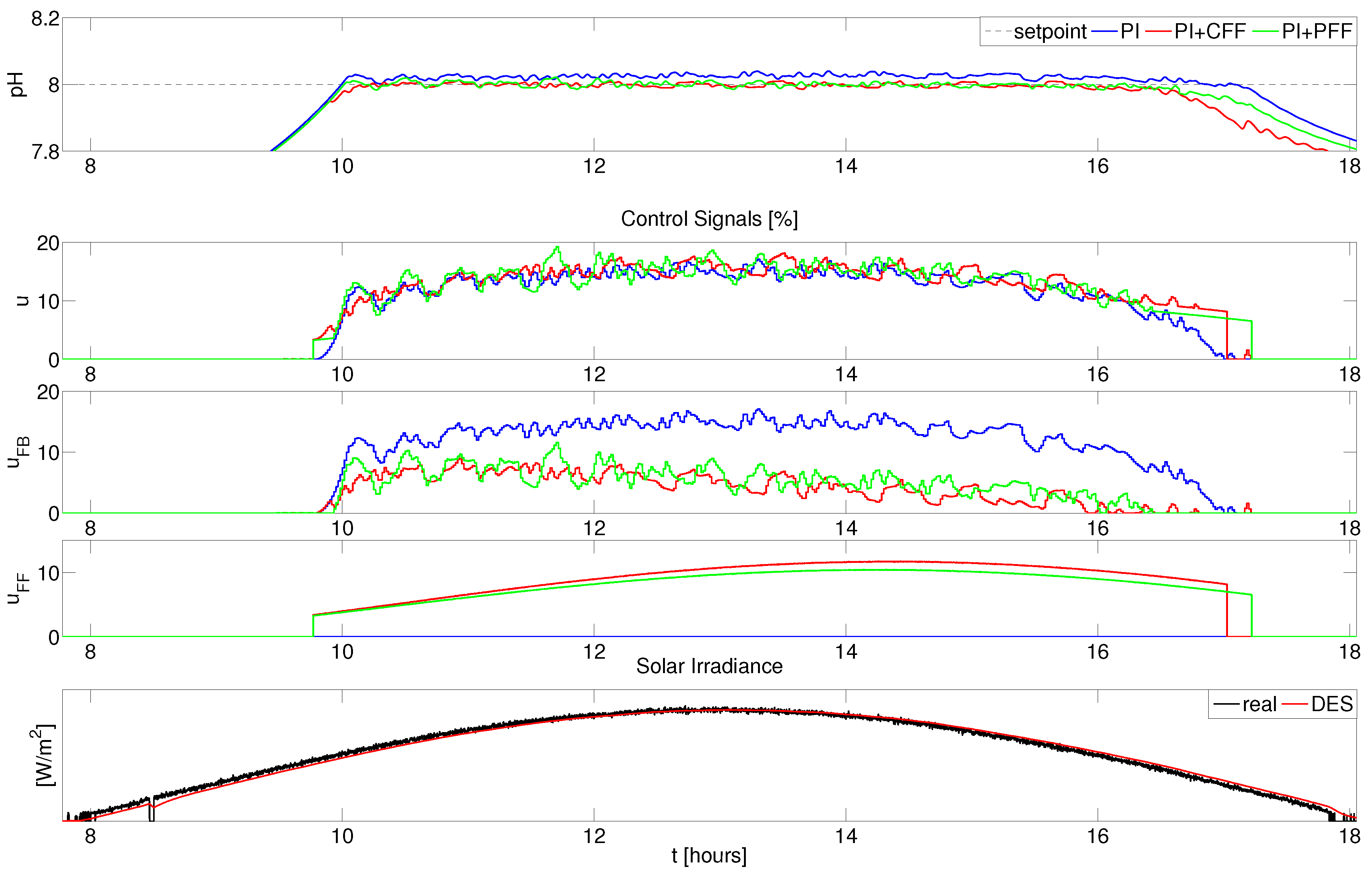
Since a graphical result for seven days and all analyzed control techniques will not allow one to see the results properly, one representative day has been selected for PI and GPC feedback controllers, which are shown in Figure 3 and Figure 4, respectively. These figures show the results of different feedforward approaches coupled with two feedback controllers in order to check the efficiency of disturbance compensation for pH process in a raceway photobioreactor. For each feedback control technique, different disturbance compensation approaches are tested and all other parameters and variables are kept unchanged. In such a configuration, the eventual changes in control performance are due to the efficacy of the disturbance attenuation, which permits us to compare different feedforward schemes.
Figure 3 shows the control results for the configuration where the PI controller is used in feedback loop. For this case, three configurations have been evaluated where disturbance compensation was performed using: feedback controller ( P I ), classical feedforward compensator P I + C F F and a predictive feedforward compensator P I + P F F . From the first plot in Figure 3, it can be seen that all tested schemes are able to maintain the pH level close to its set point. Nevertheless, the configurations using the dedicated disturbance compensator, P I + C F F and P I + P F F , obtain better precision. In these two configurations, the control signal is composed of two parts, u F F and u F B , obtained from feedforward and feedback controllers, respectively. The u F F component provided depends on the solar irradiance, and proper structure of the compensator. Moreover, from the u F F plot, it can be observed that significant differences between P I + C F F and P I + P F F are obtained. This is due to a predictive approach used in P F F that considers dead time inversion and exploits the future disturbance information estimated using the DES technique. In such a case, the estimated future values of the solar irradiance (see red plot on bottom graph in Figure 3) has an offset in comparison to the real solar irradiance signal. Notice that, in the schemes with feedforward compensators, the resulting control signal from the compensator is applied only if the pH level is bigger than 7.9; otherwise, it is set to zero. This condition is set to prevent CO 2 injections when pH is below the set point.
From the obtained results, it can be seen that none of the analyzed compensators are able to completely attenuate the disturbance effect. Even the P F F approach with future disturbance compensation does not achieve the complete attenuation. This is mainly due to two reasons. The first one is related with plant-model mismatch and the second can be linked with future disturbance estimation errors. Both factors are making the predictive disturbance compensator less effective in comparison to the nominal case where no modelling and estimation errors are considered. However, the P F F performance is better in comparison to the classical approach, which is confirmed by the indexes related to control accuracy and process performance.
The average performance indexes for the previously analyzed configurations are summarized in Table 1. The I A E index shows that the best accuracy, for the analyzed seven-day period, is obtained for P F F . On the other hand, the C F F approach improves the I A E measure in comparison to the configuration where only the feedback controller is used to compensate the disturbances. Additionally, the P F F configuration obtains the lowest I A U measure, being the most effective in control resource utilization. The improved accuracy of the approaches with feedforward compensators is obtained at the expense of higher control signal variability, which is shown by the C S E index where P F F obtains the biggest value. Besides that, the predictive feedforward compensator uses the lowest amount of the flue gases (see G a s index) from all tested configurations, being the most energy efficient.
From the process performance point of view, application of feedforward compensators improves the overall productivity of the biomass, which is confirmed through C b and P O 2 measures. The P F F configuration provides the best growth conditions, keeping the pH value close to its reference for a longer time. The photosynthesis rate increments were shown using P O 2 measure provided by the nonlinear model. This index reflects the oxygen concentration and it is proportional to the photosynthesis rate. The P O 2 increased 5.6% for the P F F configuration when compared to the C F F technique. Similar improvements are obtained in terms of energy savings. The changes in energy required for control purposes are calculated using the G a s index. This measure expresses the volume of the flue gases used during the seven-day time period. The energy usage for the microalgae production in the raceway reactor is mainly related to the energy consumed by the flue gas compressor. Based on this issue, a direct relation between G a s and energy used can be established. The reduced amount of gas usage by the control scheme has a proportional impact on the energy savings. In this case, the P F F based scheme reduced the energy usage about 4.5% regarding the C F F . These facts are crucially important for biomass production from microalgae since they increase the process rentability.
The results for the second control scenario, where the GPC algorithm is used as a feedback controller are shown in Figure 4. As in the previously analyzed scheme, the P F F compensator combined with the GPC controller provides the most accurate control of the pH. In such a configuration, the pH value is controlled close to its reference and the signal is characterized by reduced oscillations. The GPC standard intrinsic disturbance compensator, I F F , is able to improve the performance of the stand-alone GPC, but, due to design compromises (co-design trade-off between feedback and feedforward), it is less effective than the proposed predictive feedforward compensator. This fact is even more visible when the stand-alone GPC configuration is analyzed. In this case, the disturbance compensation is performed through a feedback loop, since no additional compensator is included. The disturbance compensation oriented design (allowing quick change in control signal) results in overshoot in the initial stage of the day [20]. Notice that, in all analyzed configurations, the feedback controller has the same tuning, and the disturbance compensation technique consideration improves the performance. In such a case, the best accuracy is obtained for the G P C + P F F configuration. When the control signal is analyzed for all tested configurations (plots two, three and four in Figure 4), it can be observed that the predictive feedforward compensator is starting before other configurations. This is mainly due to the predictive mechanism that is able to handle future disturbance providing the disturbance attenuation before its effect appears on the controlled variable. Additionally, the possibility for optimal adjustment of the control signal weighing factor λ is another element that has influence on control signal changes. It should be highlighted that P F F configuration in nominal cases (no modelling and disturbance estimation errors) should be able to attenuate completely the effect of disturbance [12]. In industrial practice, it will be impossible to meet this condition and consequently one can not expect perfect compensation of the measurable disturbances. Nevertheless, significant improvements in control performance regarding classical approach can be obtained as shown in the analyzed case.
Table 2 summarizes the control performance indexes for a scheme where the GPC controller is used in the feedback loop. In this case, the lowest value of I A E is obtained by the G P C + P F F . The I F F scheme improves stand-alone GPC, but it is less accurate in pH regulation than the predictive feedforward compensator. Moreover, it can be observed that configurations with disturbance compensation mechanism reduce the control effort, I A U , which has positive impact on the CO2 usage. For the C S E index, similar behavior as the previously analyzed scheme was observed. The configurations with disturbance compensation technique provide the control signal that is characterized by increased variability, whereas the control signal from P F F obtains the biggest C S E index value. From all tested configurations, the best growth conditions were obtained for P F F , which improves P O 2 index about 6.4% in comparison to the I F F . Moreover, stand-alone GPC was characterized by the biggest consumption of the control resources ( G a s ). The smallest usage of flue gases was obtained by P F F configuration. As a consequence, the predictive feedforward compensator is the most energy efficient approach, reducing it about 3.8% in comparison to the I F F scheme. This fact is of great importance in raceway photobioreactor biomass production, since it allows the possibility to reduce the process maintenance costs.
On the other hand, application of measurable disturbance compensation techniques has a positive influence on the photobioreactor productivity, which is represented by the C b measure. From this index, it can be observed that the highest productivity is achieved for P F F , improving the stand-alone GPC algorithm as well as I F F configuration. In such a case, C b has increased about 9%. This improved productivity is obtained with lower control resources utilization having a positive impact on the process performance.
From the obtained results, for both feedback control techniques, it can be deduced that the predictive feedforward compensator can provide better performance than the classical approach. Nevertheless, its final performance will depend on plant model mismatch and disturbance estimation accuracy. As shown in the previous analysis, the predictive feedforward compensator can handle measurable disturbance in a more efficient way in comparison to the classical feedforward compensator as well as GPC with intrinsic compensation. This realistic evaluation considered aforementioned issues for the pH control problem in the raceway photobioreactor, where important benefits for this particular process were obtained. Independently on the feedback controller, the application of predictive feedforward compensator results in an improved photosythesies rate, providing an average increase of 6% , and where the biomass concentration was increased about 4%. At the same time, the average energy usage was reduced about 4%.

5. Conclusions

In this paper, the evaluation of a predictive feedforward compensator and its combination with the PID and the MPC techniques were presented. The analysis was performed through a simulation study, where the pH control problem in a raceway photobioreactor was considered. To show the properties of the analyzed technique, several feedforward compensators have been considered. Through those configurations, it was demonstrated that significant improvements were obtained in control accuracy when a predictive feedforward compensator is used. In such a case, the effectiveness of the analyzed feedforward scheme was verified, obtaining significant improvements in control system performance indexes when compared to classical compensators. The positive impact of predictive feedforward compensator was also confirmed through microalgae growth performance indicators. For this particular process, it was possible to improve the photosynthesis rate about 6% and biomass concentration was increased about 4%. Moreover, the predictive compensator provides a possibility to reduce the energy required for process operation while simultaneously providing a more efficient way for the flue gas usage (used as CO 2 source). The average energy demand was decreased about 4% when a predictive compensator was used.
Based on the obtained results, it was demonstrated that application of a predictive feedforward compensator has a positive impact on the analyzed process performance, even in the presence of modelling and disturbance estimation errors.

Acknowledgments

This work has been partially funded by the following projects: DPI2014-55932-C2-1-R, DPI2014-55932-C2-2-R, DPI2014-56364-C2-1-R and DPI2012-31303 financed by the Spanish Ministry of Economy and Competitiveness and EU-ERDF (European Regional Development Fund) funds); and the UNED (Universidad Nacional de Educación a Distancia) through a postdoctoral scholarship.

Author Contributions

All authors have participated in the research summarized in this manuscript, providing development ideas, establishing design methodology, as well as evaluation strategy and analysis of obtained results. All authors have been involved in preparation of the manuscript.

Conflicts of Interest

The authors declare no conflict of interest.

References

  1. Åström, K.; Hägglund, T. Advanced PID Control; ISA Press: Research Triangle Park, NC, USA, 2006. [Google Scholar]
  2. Guzmán, J.L.; Hägglund, T. Simple tuning rules for feedforward compensators. J. Process Control 2011, 21, 92–102. [Google Scholar] [CrossRef]
  3. Veronesi, M.; Visioli, A. Automatic tuning of feedforward controllers for disturbance rejection. Ind. Eng. Chem. Res. 2014, 53, 2764–2770. [Google Scholar] [CrossRef]
  4. Hast, M.; Hägglund, T. Design of optimal low-order feedforward controllers. In Proceedings of the 2nd IFAC Conference on Advances in PID Control, Brescia, Italy, 28–30 March 2012. [Google Scholar]
  5. Rodríguez, C.; Normey-Rico, J.E.; Guzmán, J.L.; Berenguel, M. Robust design methodology for simultaneous feedforward and feedback tuning. IET Control Theory Appl. 2016, 10, 84–94. [Google Scholar] [CrossRef]
  6. Li, X.; Liu, S.; Tan, K.K.; Wang, Q.G.; Cai, W.J. Predictive feedforward control. In Proceedings of the 12th IEEE International Conference on Control & Automation (ICCA), Kathmandu, Nepal, 1–3 June 2016. [Google Scholar]
  7. Mercorelli, P. A switching Kalman Filter for sensorless control of a hybrid hydraulic piezo actuator using MPC for camless internal combustion engines. In Proceedings of the IEEE International Conference on Control Applications, 3–5 October 2012; pp. 980–985. [Google Scholar]
  8. Pawlowski, A.; Guzmán, J.L.; Rodríguez, F.; Berenguel, M.; Sánchez, J. Application of time-series methods to disturbance estimation in predictive control problems. In Proceedings of the IEEE Symposium on Industrial Electronics, Bari, Italy, 4–7 July 2010. [Google Scholar]
  9. Pawlowski, A.; Guzmán, J.L.; Rodríguez, F.; Berenguel, M.; Normey-Rico, J.E. Predictive control with disturbance forecasting for greenhouse diurnal temperature control. In Proceedings of the 18th World Congress of IFAC, Milan, Italy, 28 August–2 September 2011. [Google Scholar]
  10. Elso, J.; Gil-Martínez, M.; García-Sanz, M. Quantitative feedback-feedforward control for model matching and disturbance rejection. IET Control Theory Appl. 2013, 7, 894–900. [Google Scholar] [CrossRef]
  11. Shridhar, R.; Cooper, D.J. A tuning strategy for unconstrained SISO Model Predictive Control. Ind. Eng. Chem. Res. 1997, 36, 729–746. [Google Scholar] [CrossRef]
  12. Pawlowski, A.; Rodríguez, C.; Guzmán, J.L.; Berenguel, M.; Dormido, S. Predictive feedforward compensator for dead-time processes. In Proceedings of the 20th World Congress of IFAC, Toulouse, France, 20 October 2017. [Google Scholar]
  13. Pawlowski, A.; Guzmán, J.L.; Normey-Rico, J.E.; Berenguel, M. Improving Feedforward Disturbance Compensation Capabilities in Generalized Predictive Control. J. Process Control 2012, 22, 527–539. [Google Scholar] [CrossRef]
  14. Pawlowski, A.; Mendoza, J.L.; Guzmán, J.L.; Berenguel, M.; Acién, F.G.; Dormido, S. Selective pH and dissolved oxygen control strategy for a raceway reactor within an event-based approach. Control Eng. Pract. 2015, 44, 209–218. [Google Scholar] [CrossRef]
  15. Costache, T.A.; Acién, F.G.; Morales, M.M.; Fernández-Sevilla, J.M.; Stamatin, I.; Molina, E. Comprehensive model of microalgae photosynthesis rate as a function of culture conditions in photobioreactor. Appl. Microbiol. Biotechnol. 2013, 97, 7627–7637. [Google Scholar] [CrossRef] [PubMed]
  16. Pawlowski, A.; Fernández, I.; Guzmán, J.L.; Berenguel, M.; Acién, F.G.; Dormido, S. Event-based Selective Control Strategy for Raceway Reactor: A simulation study. In Proceedings of the 11th IFAC Symposium on Dynamics and Control of Process Systems, including Biosystems—DYCOPS-CAB 2016, Trondheim, Norway, 6–8 June 2016. [Google Scholar]
  17. De Godos, I.; Mendoza, J.L.; Acién, F.G.; Molina, E.; Banks, C.J.; Heaven, S.; Rogalla, F. Evaluation of carbon dioxide mass transfer in raceway reactors for microalgae culture using flue gases. Bioresour. Technol. 2014, 153, 307–314. [Google Scholar] [CrossRef] [PubMed]
  18. Pawlowski, A.; Mendoza, J.L.; Guzmán, J.L.; Berenguel, M.; Acién, F.G.; Dormido, S. Effective utilization of flue gases in raceway reactor with event-based pH control for microalgae culture. Bioresour. Technol. 2014, 170, 1–9. [Google Scholar] [CrossRef] [PubMed]
  19. Bernard, O. Hurdles and challenges for modelling an control of microalgae for CO2 mitigation and biofuel production. J. Process Control 2011, 21, 1378–1389. [Google Scholar] [CrossRef]
  20. Pawlowski, A.; Rodríguez, C.; Guzmán, J.L.; Berenguel, M.; Dormido, S. Measurable disturbances compensation: Analysis and tuning of feedforward techniques for dead-time processes. Processes 2016, 4, 12. [Google Scholar] [CrossRef]
  21. Fernández, I.; Acién, F.G.; Guzmán, J.L.; Berenguel, M.; Mendoza, J.L. Dynamic Model of an Industrial Raceway Reactor for Microalgae Production. Algal Res. 2016, 17, 67–78. [Google Scholar] [CrossRef]
  22. Guzmán, J.L.; Hägglund, T.; Åström, K.J.; Dormido, S.; Berenguel, M.; Piguet, Y. Feedforward control concepts through interactive tools. In Proceedings of the 18th IFAC World Congress, Milano, Italy, 28 August–2 September 2011. [Google Scholar]
  23. Camacho, E.F.; Bordóns, C. Model Predictive Control; Springer: London, UK, 2007. [Google Scholar]
  24. Hernández-Hernández, C.; Rodríguez, F.; Moreno, J.C.; da Costa Mendes, P.R.; Normey-Rico, J.E.; Guzmán, J.L. The Comparison Study of Short-Term Prediction Methods to Enhance the Model Predictive Controller Applied to Microgrid Energy Management. Energies 2017, 10, 884. [Google Scholar] [CrossRef]
  25. Mendoza, J.L.; Granados, M.R.; de Godos, I.; Acién, F.G.; Molina, E.; Banks, C.J.; Heaven, S. Fluid-dynamic characterization of real-scale raceway reactors for microalgae production. Biomass Bioenergy 2013, 54, 267–275. [Google Scholar] [CrossRef]
  26. Acién, F.G.; García, F.; Chisti, Y. Photobioreactors: Light regime, mass transfer, and scaleup. Prog. Ind. Microbiol. 1999, 35, 231–247. [Google Scholar]
  27. Acién, F.G.; Fernández, J.M.; Molina, E. Photobioreactors for the production of microalgae. Rev. Environ. Sci. BioTechnol. 2013, 12, 131–151. [Google Scholar] [CrossRef]
  28. Molina, E.; Sevilla, J.M.; Pérez, J.A.; Camacho, F.G. A study on simultaneous photolimitation and photoinhibition in dense microalgal cultures taking into account incident and averaged irradiances. J. Biotechnol. 1996, 45, 59–69. [Google Scholar]
  29. Camacho, F.; Acién, F.; Sánchez, J.; García, F.; Molina, E. Prediction of dissolved oxygen and carbon dioxide concentration profiles in tubular photobioreactors for microalgal culture. Biotechnol. Bioeng. 1999, 62, 71–86. [Google Scholar]
  30. Berenguel, M.; Rodríguez, F.; Acién, F.G.; García, J.L. Model predictive control of pH in tubular photobioreactors. J. Process Control 2004, 14, 377–387. [Google Scholar] [CrossRef]
  31. Skogestad, S. Simple analytic tuning rules for model reduction and PID controller tuning. J. Process Control 2003, 13, 291–309. [Google Scholar] [CrossRef]
Figure 1. Feedback plus feedforward control scheme.
Energies 11 00123 g001
Figure 2. Raceway reactor. (a) scheme (top and side view); (b) modelled experimental facilities.
Energies 11 00123 g002
Figure 3. Control results for PI (Proportional-Integral) as feedback controller and different feedforward approaches.
Energies 11 00123 g003
Figure 4. Control results for GPC as the feedback controller and different feedforward approaches.
Energies 11 00123 g004
Table 1. Average performance indexes for PI as feedback controller and different configurations of feedforward control schemes for the seven-day period.
Feedforward IAE IAU CSE Gas C b PO 2
Scheme[−]103[−]104[−][m3][kg/m3][kg O 2 /m3s]
-4.9833.7731476.280.4990.0278
CFF4.8723.7061936.170.5140.0285
PFF4.7133.4212125.960.5290.0301
Table 2. Average performance indexes for GPC as the feedback controller and different configurations of feedforward control schemes for a seven-day period.
Feedforward IAE IAU CSE Gas C b PO 2
Scheme[−] 10 3 [−] 10 4 [−][m3][kg/m3][kg O 2 /m3s]
-4.7413.52225.45.890.5210.0297
IFF4.6723.48533.75.800.5470.0309
PFF4.5383.39758.55.640.5710.0329

