Net Power Coefficient of Vertical and Horizontal Wind Turbines with Crossflow Runners

Abstract

The feasibility of using crossflow runners as single rotors in vertical-axis wind turbines (VAWT) or as blades in horizontal-axis wind turbines (HAWT) is numerically studied. A computational fluid dynamics model is validated from data obtained in a wind tunnel. Three crossflow runners with different number of blades are tested. Values of drag, lift and torque coefficients are numerically obtained at different turning velocities. Power coefficients C_p for crossflow VAWT and HAWT are calculated for different tip-speed ratios (TSR) and runner spin ratios (α). Since crossflow HAWT consume electrical energy for spinning the runners, the net power coefficient is estimated. Simulations indicate that a crossflow runner as a single rotor in VAWT should have a high solidity and work at low TSR. Crossflow runners working as blades in HAWT may achieve low drag to lift ratios but the C_p is penalized by the amount of energy required for spinning the runners. The optimum working condition of crossflow HAWT is located within a narrow band of low TSR and α reaching C_p values < 0.2 only.

1. Introduction

Wind energy technologies have experienced an important evolution over the last decades [1]. In large scale designs, the horizontal-axis wind turbine (HAWT) with a three-blade rotor offers a high aerodynamic performance, being the most suitable option for wind farms with large installed capacities [2,3]. This type of HAWT commonly starts working at wind speeds over U = 3.5 m s⁻¹ and with tip-speed ratios (TSR) in the range of 10–13 [2], where TSR is the ratio of the blade tip tangential velocity U_t to the wind speed U,

$$TSR=\frac{\Omega R}{U},$$

(1)

since U_t = Ω·R with Ω the rotor angular velocity and R the blade radius.

Different designs of small- and medium-sized wind turbines can be found with the purpose of working at other ranges of TSR values [4,5]. It is expected that designs with low cut-in speeds correspond to those with low TSR. Starting conditions with weak winds have the advantage of providing more working hours per day, since the most repeatable wind resource is found at low speeds [6]. These types of wind turbines specifically adapted to small power generation (<10 kW) become appropriate for urban areas and motorways (see, e.g., [7,8]).

Recent studies have focused on developing small-scale systems that work in the range of very low TSR (<3).

Table 1. Example of maximum power coefficients C_p of different turbine types.

TSR	Cp	Type	Turbine	Analysis	Ref.
0.3	0.45	VAWT	Crossflow runner	Numerical	[9]
0.5	0.30	VAWT	Crossflow runner	Field testing of prototype	[10]
0.7	0.47	VAWT	Savonius–Darrieus	Wind tunnel	[11]
0.8	0.26	VAWT	Savonius	Numerical	[12]
2.6	0.31	VAWT	Darrieus	Numerical	[13]
0.6	0.17	HAWT	Multi blade	Wind tunnel	[14]
1.0	0.35	HAWT	Magnus	Analytical based on wind tunnel data	[15]
2.7	0.40	HAWT	4 blades NACA2404	Wind tunnel	[16]

reports values of the maximum power coefficient (C_p, the ratio of the power extracted by the turbine to the power of the incoming flow) achieved in different turbine types working at low TSR [9,10,11,12,13,14,15,16]. Except [9,12,13], data shown in Table 1 have been obtained experimentally, with some designs offering cut-in wind speeds as low as 1.6 m s⁻¹.

Starting conditions for low wind velocities can be obtained with Magnus type turbines [17] that consist in HAWT with rotating cylinders instead of standard blades. The Magnus effect arises when a spinning cylinder is immersed in a flow and it provides a lift force that is the responsible for producing the required torque (see, e.g., [18]). Several versions of Magnus type turbines have been investigated, varying the number of spinning cylinders and their rotational speeds ω [15,18,19,20]. The performance of Magnus type turbines depends on the cylinder spin ratio α, defined as

$$\alpha =\frac{\omega D/2}{U},$$

(2)

with D the diameter of the spinning cylinders.

Sedaghat [15] has recently developed a theory for designing Magnus wind turbines with rotating cylinders working as blades in HAWT, estimating an optimum of C_p = 0.35 at TSR = 1 in the range of 1.5 < α < 2.5 (see Table 1). In comparison with plain rotating cylinders, higher values of the lift coefficient have been obtained by using spiral fins [21,22], although the lift coefficient substantially decreases as the TSR tends to zero [22]. A drawback of rotating cylinders (both plain and with spirals) is the high value of the drag to lift ratio, which contrasts with the very low ratio recently obtained with a circulating airfoil specifically designed for providing a Magnus force in HAWT [23]. However, the complexity of the previous mechanism motivates the investigation of simpler options for applications in wind energy as, for example, the use of crossflow runners.

Once a crossflow runner is immersed in a flow, it achieves an autorotation regime (or free spin regime α_f). The air flow is able to spin the runner from the fully stopped condition (α = 0) to the free regime (α = α_f) by varying an external load (that extracts mechanical energy) applied to the shaft of the runner. Thus, the crossflow runner may be used as a single rotor in vertical-axis wind turbine (VAWT) when working in the α_f ≤ α ≤ 0 range (see

Table 2. Regimes of the crossflow runner.

Regime	Rotation *	External Energy Consumed	Use
α < αf	anticlockwise	Yes	-
αf ≤ α ≤ 0	anticlockwise	No	Single rotor in VAWT
0 < α	clockwise	Yes	As blades in HAWT

* Sense of rotation in all the figures of the present paper (e.g., anticlockwise implies ω < 0 in Equation (2)).

and Figure 1). On the other hand, external energy (not related with the incoming air flow) is required for spinning the runner at fixed angular velocities in other regimes (e.g., 0 < α). This is a proper functioning for crossflow runners that work as blades in HAWT (as in Magnus HAWT [15]; see Table 2 and Figure 1). Table 2 also indicates the sign convention of α and the sense of rotation of the crossflow runner in all the figures of the present paper.

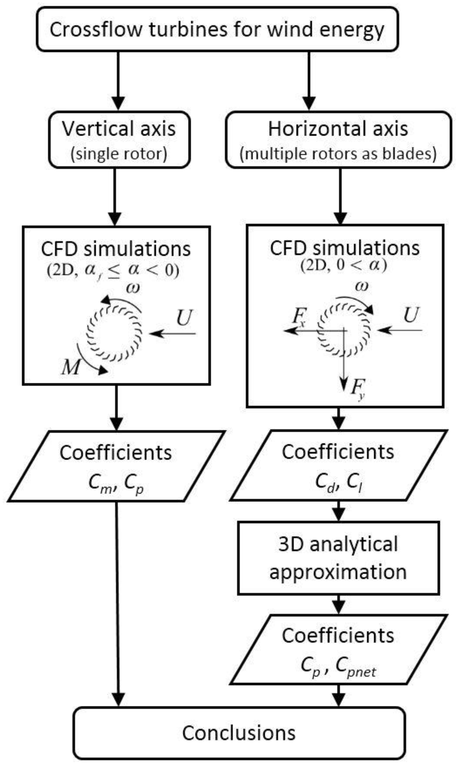
Here, the feasibility of using crossflow runners in VAWT (as a single vertical rotor) as well as in HAWT (as blades) is analyzed. The flow-process diagram of the current work follows Figure 2. Section 2 describes the experimental set up. The two-dimensional (2D) Computational Fluid Dynamics (CFD) model is explained in Section 3 and its validation is carried out in Section 4.

Once validated, the 2D CFD model is applied for analyzing the performance of a crossflow runner used in a VAWT, which means working in the α_f ≤ α ≤ 0 regime (Section 5). Values of torque (C_m) and power (C_p) coefficients are obtained and compared with those corresponding to other types of turbines. This case has already been analyzed numerically by Dragomirescu [9] for a bigger crossflow runner. In comparison with Dragomirescu [9], we provide detailed information of the behavior of a single blade and study the consequences of: (1) using flows with different Reynolds numbers; and (2) changing the orientation of the blades.

Besides, we also extend the study carried out in Dragomirescu [9] by analyzing the feasibility of using crossflow runners for working as blades in HAWT. The 2D CFD model is also applied in this configuration, which means working in the 0 < α regime (Section 6). In this case, lift (C_l) and drag (C_d) coefficients of the spinning cylinders are calculated and used in a 3D analytical approximation (based on [15]) for estimating the C_p value as a function of TSR and α. In addition, we develop a formulation for estimating the net power coefficient that takes into account the power needed for spinning the runners in HAWT. Finally, Section 7 contains the main conclusions of the present paper.

2. Experimental Set Up

Experimental data are obtained with the closed circuit wind tunnel of the Energy Laboratory at the University of Girona. Figure 3 shows a picture of the facility. The wind tunnel has total dimensions of 7300 mm × 3600 mm × 1800 mm (length × height × width) with a test section made of transparent glass of dimensions 395 mm × 395 mm (cross-section) and 1325 mm (length). The ducts of the vertical wind tunnel are made of galvanized steel with internal corner vanes. The settling chamber prior to the contraction cone contains an aluminum honeycomb and a screen to straighten the flow direction. The contraction cone is wooden made and it is internally fixed to the outer panels. The design of these elements follows the technical note of Mehta and Bradshaw [24]. An axial flow fan (HM 80 T 4 model, Casals, Camprodon, Spain) is controlled with a variable-frequency drive (Altivar 312 model, Schneider Electric, Rueil-Malmaison, France; 0–50 Hz), which provides a maximum speed of 40 m s⁻¹ at the exit of the contraction cone.

The blades of the crossflow runner are manufactured by bending a 0.2 mm thick sheet of steel. Its inner edge is situated at 24 mm from the center of rotation, with an outer diameter D = 62 mm and a transversal length to the free stream air equal to L = 180 mm (see Figure 4). The crossflow turbine is located within the channel test with its rotation axis at a distance of 435 mm from the end of the contraction cone. Three different configurations of the runner are tested. They differ in the number of blades, being 6, 11 or 22 (see Figure 4). We point out that the six blades of Prototype 3 are not evenly distributed since we built it by removing 16 blades out of the runner with 22 blades. At a given time, upstream blades are identified as those that first impact with the incident flow (i.e., those situated on the right-hand side in Figure 4 since the direction of the incoming flow U in all the figures of the present paper is from right to left).

Note that our 2D representation does not take into account the reinforcement rings of the actual runner. The rotation axle of the turbine is mounted on a strain gauge wind tunnel balance (EI400 Series model, DELTALAB, Carcassonne, France, resolution of 0.01 N, accuracy of ±1%) to measure lift and drag forces.

The fluid flow behavior is acquired by means of a Particle Image Velocimetry (PIV) technique. We use a 2D PIV system of Dantec Dynamics (Skovlunde, Denmark) with a FlowSense camera and a DualPower laser Nd:Yag of 532 nm, 120 mJ/pulse and 14.8 Hz. The laser is fixed vertically with a downwards light beam to be able to light up a longitudinal plane across the channel test at 140 mm from one end of the turbine (in order to avoid the middle reinforcement ring). Seeding particles are introduced at the end of the channel test by a smoke generator (Magnum 650 EU model, Martin, Arhus, Denmark). We use the DynamicStudio software (Dantec Dynamics, Skovlunde, Denmark) for configuring, acquiring and analyzing data after synchronizing the system with the turning velocity of the runner. This value is measured with a laser tachometer (ST-6234B model, Reed Instruments, Wilmington, NC, USA, resolution of 0.1 rpm, accuracy of ±0.5% + 1 digit). At the same time, the air flow velocity U is independently measured in the channel test with an anemometer (Master 8901 model, Dwyer, Michigan, IN, USA, resolution of 0.01 m s⁻¹, accuracy of ±2%).

Figure 5 shows the schematics of the experimental system, where point A indicates periodicity. In summary, the experiment consists in: (1) fixing the frequency value in the variable speed drive connected to the fan; (2) measuring the turning velocity of the crossflow runner under free spinning conditions; (3) synchronizing the PIV system according to the runner’s spinning velocity; and (4) acquiring PIV data, wind tunnel balance data and wind speed data. This procedure is repeated for various wind speed values and configurations of the turbine (6, 11 and 22 blades).

3. Simulation Set Up

Several researchers have applied the CFD technique for studying the interaction of flows with rotating blades [25,26,27,28,29,30,31]. Here, simulations are carried out with ANSYS-Fluent (ANSYS, Inc., Canonsburg, PA, USA) in a configuration very similar to that successfully employed in [9]. This commercial CFD software has been widely applied in the simulation of air flows in complex cases involving wind turbines with remarkable success [30]. For simplicity, simulations are done in 2D along the plane that is experimentally analyzed with the PIV technique. Air properties are density ρ = 1.225 kg m⁻³ and absolute viscosity µ = 1.7894 × 10⁻⁵ Pa s.

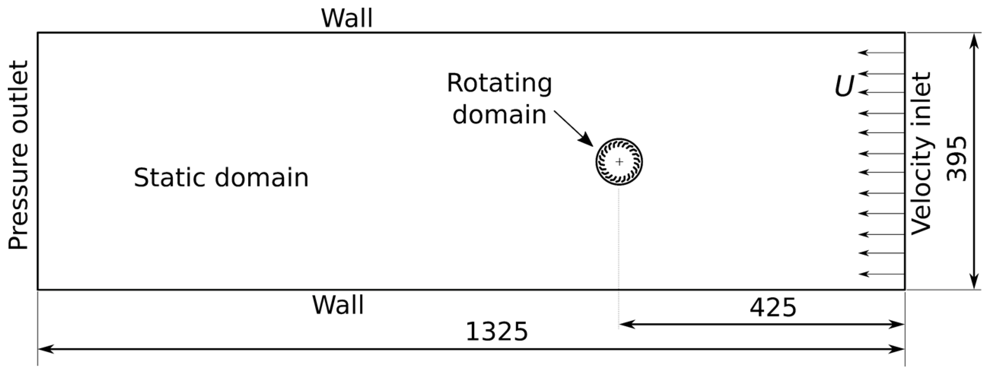
The computational domain is divided into two parts: a static domain and a rotating one that contains the blades of the turbine (see Figure 6). The inner boundaries of the static domain coincide with the outer boundaries of the rotating domain, whereas the external boundaries of the static domain correspond to the limits of the channel test. A transient simulation with a sliding mesh technique for the rotating domain is adopted.

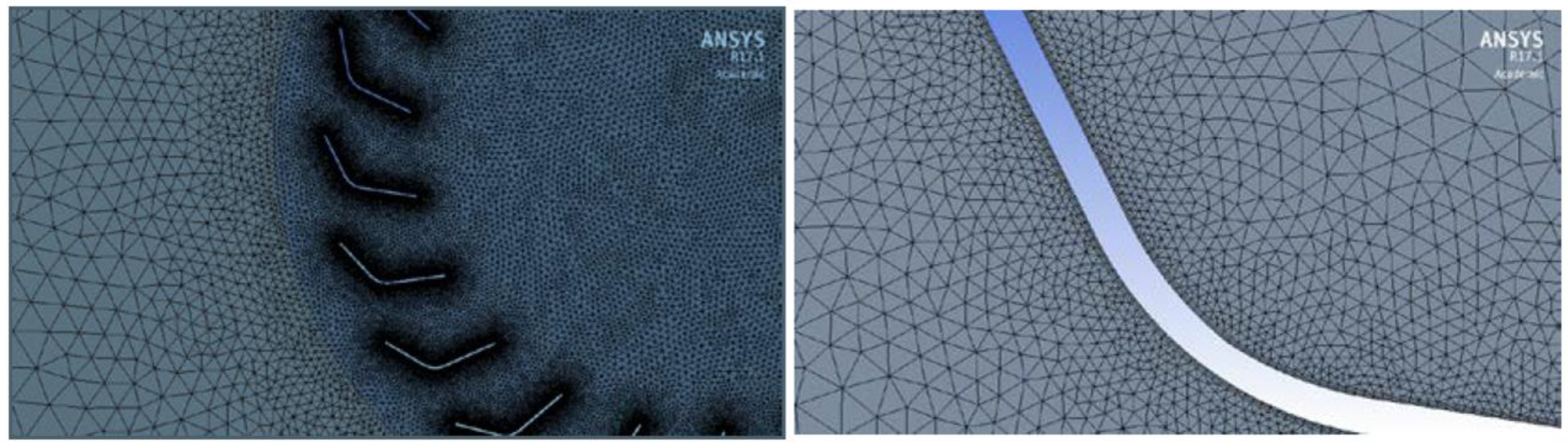
The mesh is created with ANSYS-Meshing (ANSYS, Inc., Canonsburg, PA, USA). Three layers of quadrilaterals (since the mesh is 2D) are used around the blades with triangles in the rest of the computational domain (see Figure 7). The edge size of the elements at the blades is 0.05 mm with a growth rate equal to 1.2. The maximum length of the edges of the elements is equal to 0.5 mm in the rotating domain and 5 mm in the static one. A total amount of 284,012 elements is needed for meshing the 2D domain. For this mesh, the y+ values on the blades are calculated with the function specifically defined for this purpose in the CFD-Post software. The maximum value of y+ (y+_max) for the U = 10 m s⁻¹ case varies from 1.79 for a turbine rotating at 1500 rpm anticlockwise to 0.99 rotating at 750 rpm clockwise. Weaker air free stream conditions lead to smaller values of y+_max. For example, for U = 2 m s⁻¹, y+_max ranges from 0.58 for a turbine rotating at 500 rpm anticlockwise to 0.33 rotating at 200 rpm clockwise. Two coarser meshes are also simulated for studying the sensitivity of the results to the mesh size, as detailed in the next section.

The transient numerical model uses a time step Δt that provides a turn of 1° of the turbine for any value of the angular velocity (Δt = 1/(6N) with N the turbine’s turning velocity in rpm). For comparison purposes, simulations applying a Δt equivalent to a 0.2° turn of the 22 blades turbine were carried out for different values of N and results did not significantly vary (changes in forces less than 0.5%). The numerical algorithm solves the momentum and mass conservation equations with a double precision pressure-based algorithm and second order discretization schemes. The shear stress transport (SST) k-ω turbulent model is chosen, as successfully done in [23] for similar conditions, and the pressure-momentum coupling uses the pressure implicit with splitting of operator (PISO) method. Differences of our numerical set up with [9] are that, here: (1) we adapt the time step to have the same angle of rotation per outer iteration for all the cases analyzed; (2) our flow regime corresponds to lower Reynolds numbers (Re = UDρ/µ), as discussed in Section 5; and (3) we use the SST k-ω model as in [23] instead of the realizable k-ε model since it is expected to be more robust and accurate.

The boundary condition at the inlet is defined as a uniform velocity with a 5% of turbulence intensity and a turbulent viscosity ratio equal to 10 for all cases, both being typical values for these turbulence parameters. A lower value of turbulence intensity (=1%) at the inlet was also tested for the U = 2 m s⁻¹ and α = 0.48 case. Results deviated less than 0.7% from those obtained with a 5% turbulence intensity. A pressure equal to 0 Pa (relative) is fixed at the outlet boundary. All other boundaries are stated as smooth walls.

We apply the criterion of performing a maximum of 30 inner iterations at each time step. In some cases, the convergence criterion (residuals less than 10⁻⁴) is achieved earlier. A minimum amount of 10⁴ time steps is simulated. Values of forces and torque are monitored for the whole crossflow runner (all blades) as well as for one individual blade. After an initial time span, the behavior of forces and torque shows a periodic signal. Once we confirm that the system reaches a stationary behavior in the sense that the oscillatory signal for one individual blade does not remarkably change when shifted 360° in time, values of both x and y forces as well as torque are recorded. Since the simulation is 2D, the values of forces and torque reported by the solver are per unit length, being multiplied by L (the length of the turbine) for carrying out the comparison with experimental data.

Forces F_x (positive leftwards) and F_y (positive downwards) (see the inset of the CFD simulations box in Figure 2) are also used for calculating the aerodynamic coefficients of lift C_l and drag C_d, as usual [23]

$$C_l=\frac{F_y}{q{S}_{ref}},$$

(3)

$$C_d=\frac{F_x}{q{S}_{ref}},$$

(4)

where q = $\raisebox{1ex}{$1$}\!\left/ \!\raisebox{-1ex}{$2$}\right.$ρU² is the kinetic energy per unit volume of the incoming flow and S_ref is the reference area of the crossflow turbine (S_ref = D·L).

The torque coefficient C_m is calculated from [9]

$$C_m=\frac{M}{q{S}_{ref}D/2},$$

(5)

where M is the torque acting on the blades (value reported by the solver multiplied by L) with respect to the center of rotation of the runner.

4. CFD Validation

Here, the purpose is to assess the ability of the CFD model to correctly reproduce the observed trend of both lift and drag forces. Since the experimental set up does not include any external brake or power for modifying the rotating speed of the runner, laboratory data correspond to the free regime α_f (or autorotation) case. Autorotation cannot be observed in a plain cylinder but it arises in other types of rotors as, for example, the Savonius one [26] and the cycloidal propeller [27,28].

The angular velocity N_f (in terms of rpm) of the free regime achieved in our crossflow runners as a function of the incoming wind speed U is shown in Figure 8. Note that values of N_f are defined as negatives since runners turn anticlockwise.

The free turning velocity obtained with high to medium solidity levels (11 and 22 blades) is almost the same in the range of U < 15 m s⁻¹ as it is seen in Figure 8 (changes less than 6%). For higher wind speeds, the free turning velocity depends on the solidity of the runner, decreasing as the number of blades decreases. The crossflow runner with the largest solidity keeps a linear relationship between N_f and U (linear regression with a correlation coefficient R² = 0.998). The lowest wind speed that produces autorotation is almost the same for both 22 and 11 blade turbines (slightly below 4 m s⁻¹). As the solidity of the turbine is reduced, the lowest wind speed for achieving the free regime increases and, at the same time, the runner turning velocity becomes substantially smaller than in the other configurations. In an ideal frictionless coupling between the runner shaft and the turbine (i.e., no bearing friction forces), the lowest flow velocity that would turn the runner would tend to zero.

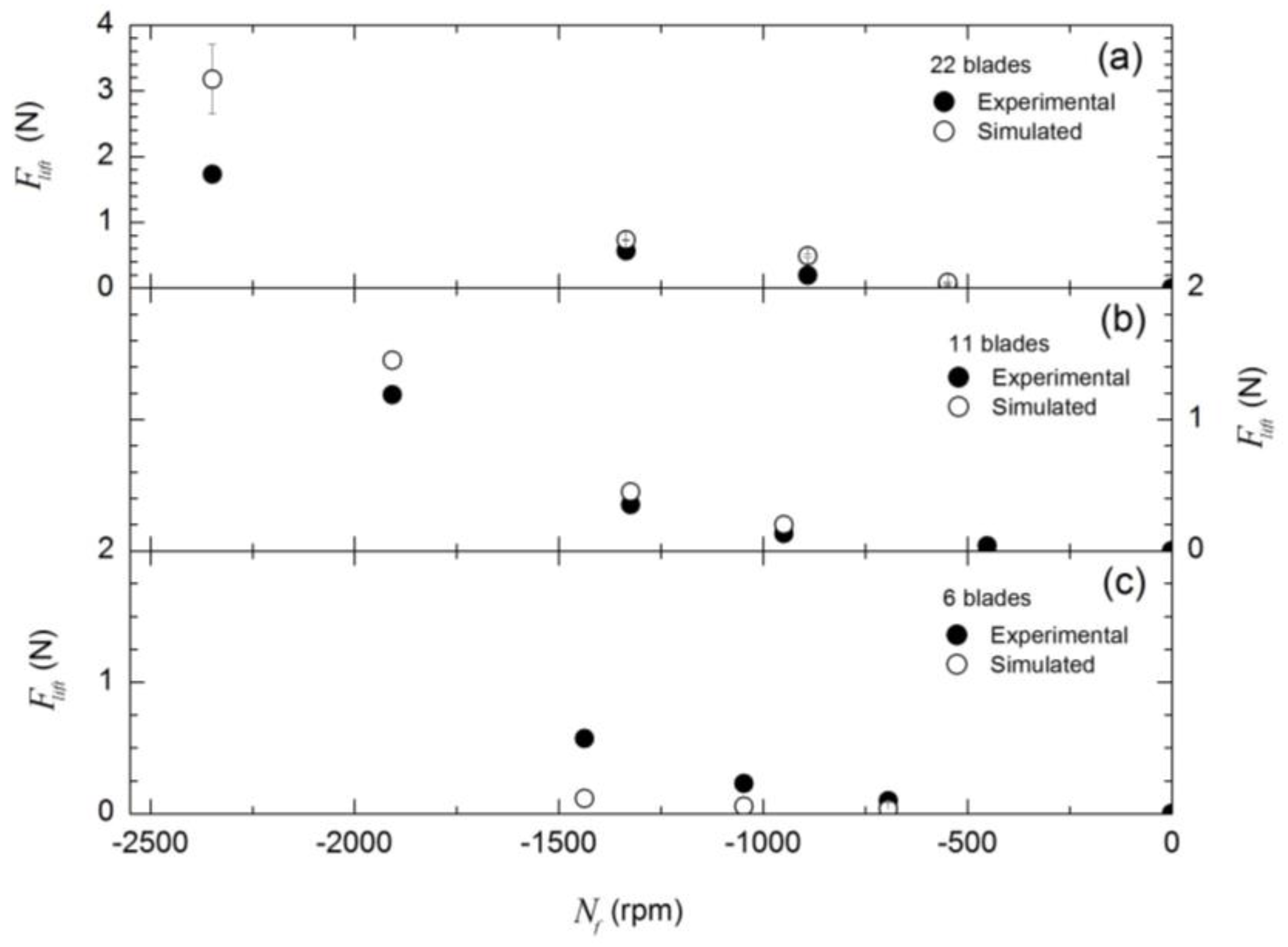
Drag F_x (positive leftwards in Figure 6) and lift F_y (positive downwards in Figure 6) forces for the free regime conditions of Figure 8 are measured and simulated (see Figure 9 and Figure 10). For U < 15 m s⁻¹ (N_f > −1500 rpm), the global trend experimentally obtained is correctly captured by the simulations. However, at very large values of U (on the order of 26 m s⁻¹, N_f < −1900 rpm), discrepancies between simulations and experiments become greater. Some reasons that may explain the over prediction of the simulation values in comparison with the experimental data are: (1) the finite effect of the actual runner geometry (end plates effect not occurring in the simulations); (2) the effect of the reinforcement rings (this geometry not included in the virtual domain simulated); and (3) unequal blades in the actual runner (out of balance).

Results in Figure 9 and Figure 10 include the uncertainty values of both measured and simulated data. The error bars of data are less than 6% for all cases and may be even lower than the size of the symbol used in the graphs. The error bars added to the simulation values correspond to the grid convergence index GCI_fine21 that is an estimation of the uncertainty produced by the discretization procedure [32]. Here, the evaluation of the GCI_fine21 index for the 22 blades runner is carried out by using three meshes that differ in the number of elements employed: a coarse mesh with 45,362 elements, a medium size mesh with 82,585 elements and a fine mesh with 284,012 elements. Grid patterns of coarse and medium meshes are identical than those for the finer mesh. The goal values for calculating the GCI_fine21 index are C_d and C_i. CFD results for the 22 blades rotor configuration under seven different scenarios with flow inlet velocities ranging from 2 m s⁻¹ to 26.5 m s⁻¹ and turning velocities ranging from −2358 rpm to 1000 rpm lead to GCI_fine21 values below 17% (C_i as a key variable) and below 8% (C_d as a key variable). Large values of the GCI_fine21 index may indicate poor grid designs. However, in four of the seven cases, the GCI_fine21 index is below 5% for C_i and in six of the seven cases, it is below 4% for C_d.

Besides quantitative values, the flow qualitative behavior was experimentally investigated. Figure 11 plots the contours of the air velocity magnitude obtained with the PIV experimental technique for different values of the incoming flow U. Blank regions correspond to those zones with no available information since they are located in the shaded zone of the laser beam. As pointed out above, the free turning velocity N_f for the three turbines (6, 11 and 22 blades) differs, increasing with U. For a weak air free stream, N_f is low and the flow tends to be symmetrical with low values of lift and drag forces, especially in low solidity runners. As N_f increases due to higher values of U, a region of low velocity situated near to the lower side of the exit of the runner is formed. This region is clearly differentiated from the rest of the wake in the runner with high solidity (Prototype 1).

The above behavior agrees with the streamlines obtained from the experimental data shown in Figure 12. At a fixed value of wind speed U, the flow pattern deviates from symmetry as the number of blades increases, especially at the wake. There, a low velocity zone at the lower left exit of the turbine is clearly observed in most of the flow speed U cases for the 22 blades rotor.

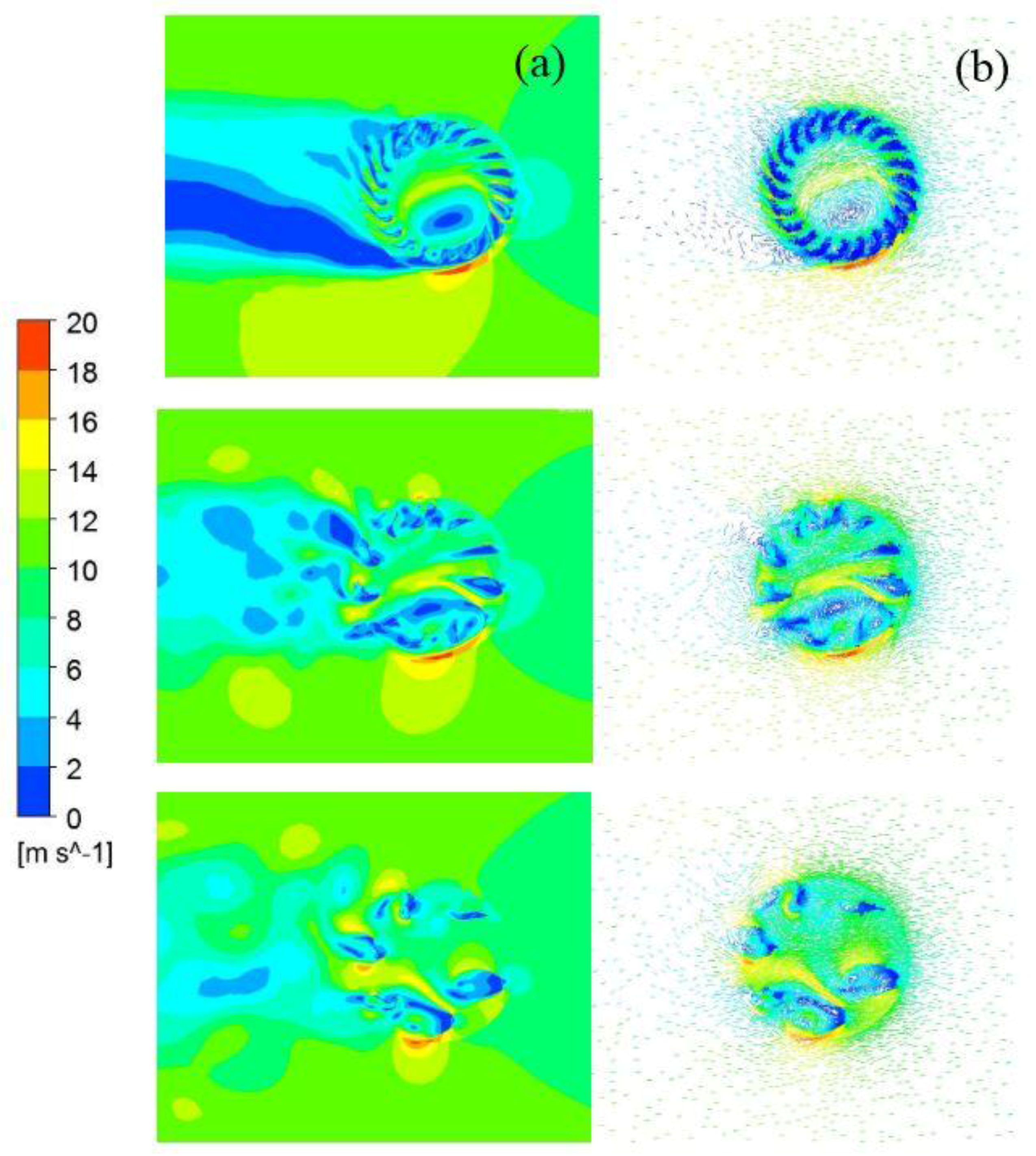
For comparison purposes with Figure 11 and Figure 12, Figure 13 shows the velocity contours and vectors simulated with ANSYS-Fluent for the U = 10 m s⁻¹ case under N_f conditions. In the high solidity configuration at high incoming velocities, there is a zone of low velocities attached to the lower exit of the turbine (confirming the observation with the PIV technique) that, at the same time, includes a vortex located inside the runner, as already pointed out in [9]. The effects of these features are discussed in Section 5.

In the upper case of Figure 13 (runner with 22 blades) a region with a significant change in the velocity field is observed in the lowermost part of the runner where opposite directions between the blade velocity (turning anticlockwise) and the incoming flow velocity are found. For this runner, a high velocity value is predicted at the blade tip exit of several upstream blades and an inner intense anticlockwise vortex is formed (confirming the results reported in [9]). This vortex is caused by the geometry of the blades since their tips point at different directions towards the inner of the runner and lead to a blockage of the incoming flow at the upstream lower zone of the runner (thereby generating an inner region of low velocity). At the lower left exit region of the runner, a series of clockwise and anticlockwise vortices is observed. This behavior is not exactly reproduced when simulating the runner with 11 blades due to its lower solidity. In this case, the flow that crosses the turbine is not intensively forced to follow an upward direction since the separation between the blades is larger than in the runner with 22 blades.

Since the simulation of the high solidity runner (22 blades) under the free regime condition satisfactorily reproduces the experimental data for U < 15 m s⁻¹, the methodology described in Section 3 is applied to study the use of crossflow runners (with 22 blades) in VAWT (Section 5) and in HAWT (Section 6).

5. VAWT

A vertical-axis single rotor crossflow runner works in the regime α_f ≤ α ≤ 0. In this case, TSR is equal to −α (since the turning velocity is negative by convention) and the performance curve of the wind turbine is achieved by braking it from the runaway condition (α = α_f) to the fully stopped one (α = 0). Simulations use flow speeds 4 m s⁻¹, 5 m s⁻¹ and 10 m s⁻¹, being above the lower speed for autorotation experimentally found for the 22 blades runner case (Figure 8).

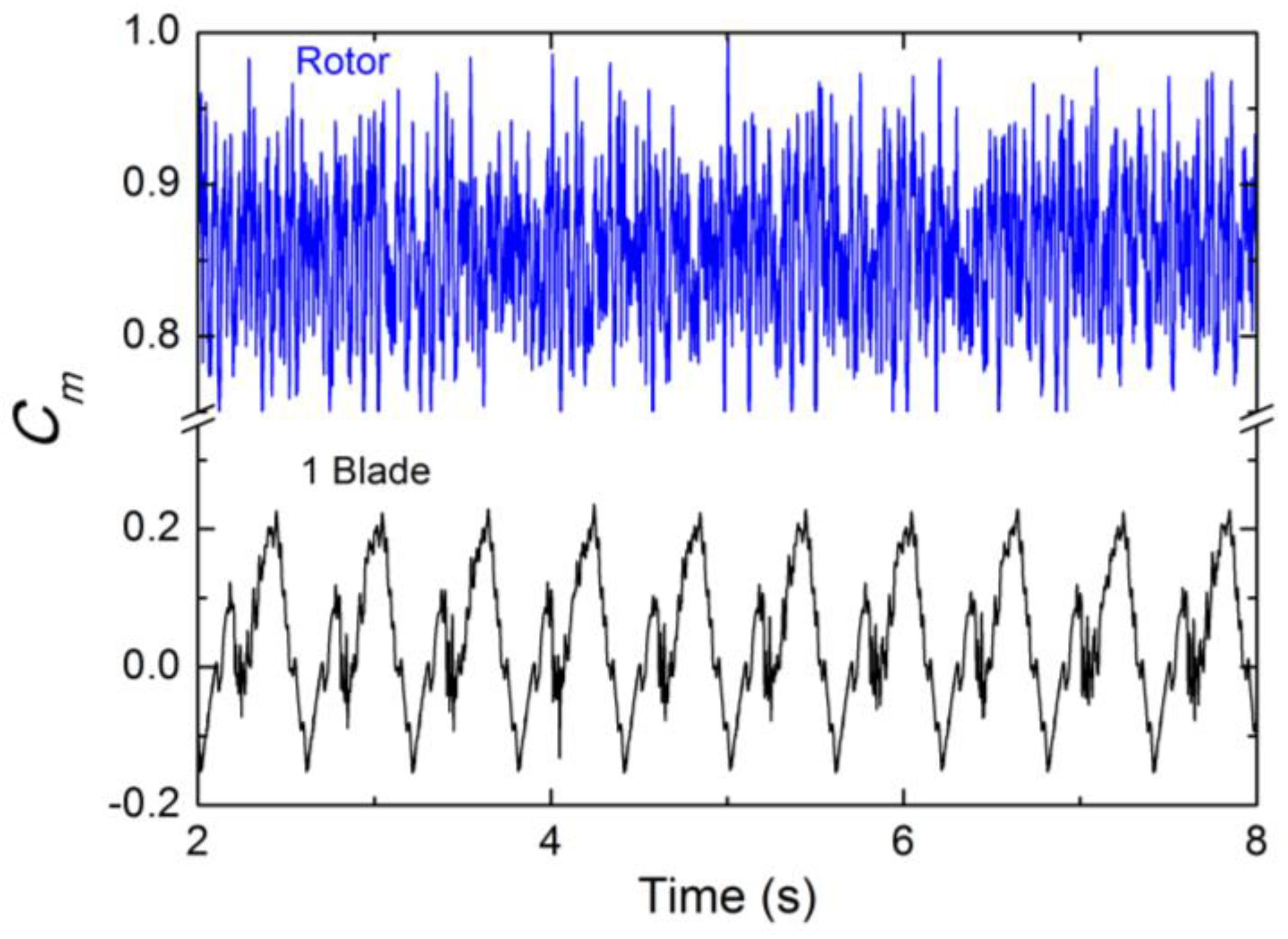
As an example of the results found, we discuss the case of U = 4 m s⁻¹ and N = −100 rpm (Re = 1.7 × 10⁴). Under these conditions, the torque coefficient C_m calculated from Equation (5) for the whole runner shows an irregular oscillatory behavior with a peak in the frequency spectrum at 36.7 Hz, which matches the blade to blade passing frequency (=−22 N/60 with N = −100 rpm; Figure 14). The behavior of C_m for the whole rotor reproduces that reported in [9] although here with a higher amplitude of the oscillations most likely due to the differences in shape and size of the blades. For a single blade, the time evolution of C_m (calculated from Equation (5) with M the torque acting on one blade with respect to the center of rotation of the runner) clearly has a signal with a frequency equal to the turning velocity (=−N/60 = 0.6 Hz with N = −100 rpm; Figure 14).

The variation of C_m as a function of the blade position is shown in Figure 15, where data correspond to the blade cycle ranging from 6.424 s to 7.024 s in Figure 14. Angle θ = 0° in Figure 15 refers to the uppermost position of the blade in Figure 4 and increases clockwise.

The pattern observed in Figure 15 can be explained from the velocity vectors and pressure contours of Figure 16. A single blade produces a maximum torque once situated in the 210° < θ < 280° range approximately (Figure 15). It coincides with the region where the position of the blade with respect to the incoming flow is suitable for generating non-negligible lift forces (high flow speed and low pressure below the blade and low flow speed and high pressure above it). This contrasts with the drag mechanism for generating torque observed in the 10° < θ < 40° region (see Figure 15 and Figure 16). Drag is also responsible of the main contribution for creating a negative torque (100° < θ < 140° in Figure 15) due to a quasi-perpendicular impact of the incoming flow on the blade surface (see Figure 16).

Typical crossflow runners in hydraulic turbines are drag-driven due to the use of a water inlet conduit that points towards a limited number of blades (becoming an impulse-type machine). Here, in contrast, the entire crossflow runner is immersed in the flow (air) and, from the above, lift is the main contributor for producing the net torque.

The flow simulation predicts the existence of a vortex in the lower left region behind the runner, whose change in intensity causes signal variations between cycles for a single blade and, consequently, for the whole runner. Although this behavior is observed for other values of U and N in the region α_f ≤ α ≤ 0, an intense vortex shedding as that found behind static cylinders at similar Re [33] is not detected.

The performance of the runner is expressed in terms of the power coefficient C_p,

$$C_p=\frac{P}{qU{S}_{ref}},$$

(6)

where P (=Ω·M) is the power extracted by the turbine.

From Equations (1) and (5), $C_p=TSR{C}_m$ where $C_m$ is obtained after averaging the simulated values during five runner rotations once the single blade data clearly indicates a periodic signal. The results of C_p are shown in Figure 17 where the values are substantially lower than those exposed in Dragomirescu [9]. This is because our turbine has a higher aspect ratio (=L/(D/2)) and a lower Reynolds number, and both effects are known to reduce efficiency in VAWT [34]. The comparison with other types of wind turbines, such as Savonius, horizontal multi-blade and horizontal three-blade, confirms that crossflow runners working as VAWT may only be suitable solutions for very low TSR values (Figure 17).

The simulations here shown do not include any resistant torque provided by shaft bearings. Therefore, positive values of C_m are reported at turning velocities beyond the runaway points experimentally obtained. Thus, crossflow runner data of C_p in Figure 17 correspond to upper bounds. We also note that our study has focused on VAWT with straight blades. However, twisted blades may enhance the power output, as already pointed out in detailed 3D numerical simulations of Savonius [35] and Darrieus rotors [36]. In addition, twisted blades substantially reduce the oscillations of torque and power, although the interactions with the vortices at the wake avoid the existence of completely smooth output signals [36]. On the other hand, curved blades along the z-direction contribute to alleviate the bending moments of straight blades, although oscillations of torque and power similar to those of the straight blade case are also expected [36].

The effect of modifying the orientation of the blades has also been investigated. Three rotors, each one with 22 blades of equal shape to those used in Figure 4 but inclined to form a blade tip exit angle of 20.5°, 30.5° and 35.5° (the nominal blade tip exit angle is 25.5°; see Figure 4c), have been simulated at Re = 1.7 × 10⁴ and different TSR. Results are shown in

Table 3. Torque and power coefficients as a function of the blade orientation angle. All cases use a 22-blade rotor with U = 2 m s⁻¹ (Re = 1.7 × 10⁴).

	TSR = 0.08		TSR = 0.16
Blade Tip Exit Angle	Cm	Cp	Cm	Cp
20.5°	0.798	0.065	0.692	0.112
25.5°	0.857	0.070	0.723	0.117
30.5°	0.896	0.073	0.730	0.118
35.5°	0.846	0.069	0.687	0.112

. For all the cases analyzed, the power coefficient is maximum when using the 30.5° configuration, with a 12% increase in comparison with the 20.5° case (TSR = 0.08, turning velocity equal to 100 rpm). However, differences reduce at 6% only for higher TSR values (TSR = 0.16, turning velocity equal to 200 rpm). Results indicate that as the turning velocity increases, the optimum value of the blade tip exit angle shifts towards smaller values.

6. HAWT

Spinning crossflow runners mounted as blades in horizontal-axis turbines work in the regime 0 < α (see Table 2 and Figure 2) so the energy required for spinning them must be externally supplied (by an electrical motor, for example). The net lift over the runner provides the force that generates the torque for rotating the blades around the center of the hub (see Figure 1). Here, the aerodynamic coefficients C_l and C_d, rather than the torque coefficient C_m, determine the performance of the turbine.

The 2D behavior of the 22-blade crossflow runner is investigated with ANSYS-Fluent for incoming flow velocities U = 2 m s⁻¹, 5 m s⁻¹ and 10 m s⁻¹ and spinning turning speeds from 0 to 500 rpm at 100 rpm intervals (turning clockwise; that contrasts with Section 4 and Section 5 where the runner turned anticlockwise). As an example of the results found, the N = 300 rpm and U = 2 m s⁻¹ (Re = 8489) case is discussed. For this case, Figure 18 shows drag and lift coefficients of the 22 blades as a function of time.

The frequency analysis of the signal of Figure 18 reveals a dominant peak at 10 Hz with harmonics of decreasing amplitude that exhibit a secondary peak at 110 Hz. The latter corresponds to the blade to blade passing frequency (f = 22N/60 with N = 300 rpm) of the crossflow runner whilst the 10 Hz value is related to the signal of the oscillating flow past the runner as described next.

Figure 19 shows the pressure field at 0.04 s time intervals starting at 9.11 s and ending at 9.21 s. The pressure pattern clearly indicates the existence of a vortex shedding at the upper left exit of the runner. A frequency analysis by means of the Fast Fourier Transform of the pressure signal at the point located D/2 downstream from the center of rotation and D/4 above it confirms a maximum peak at frequency f = 9.9 Hz, followed with harmonics and a secondary peak at the blade to blade passing frequency (110 Hz) (see Figure 20). As expected, the 110 Hz peak is much narrower than that corresponding to the signal of the vortex shedding due to the inherent variability of the latter signal. The Strohual number of the vortex shedding is St = fD/U = 0.31 that for α = 0.49 is close to the condition of the first shedding mode in alternate vortex detected in circular cylinders (although for higher Re number [23]).

The time evolution of drag and lift coefficients for a single blade of the crossflow runner (Figure 21) clearly has a periodic signal with a frequency equal to that of the turning velocity N/60 (=5 Hz for the N = 300 rpm case). Besides this dominant peak, the frequency analysis (not shown) reveals a secondary peak at 10 Hz corresponding to the dominant frequency of the vortex shedding observed in Figure 19.

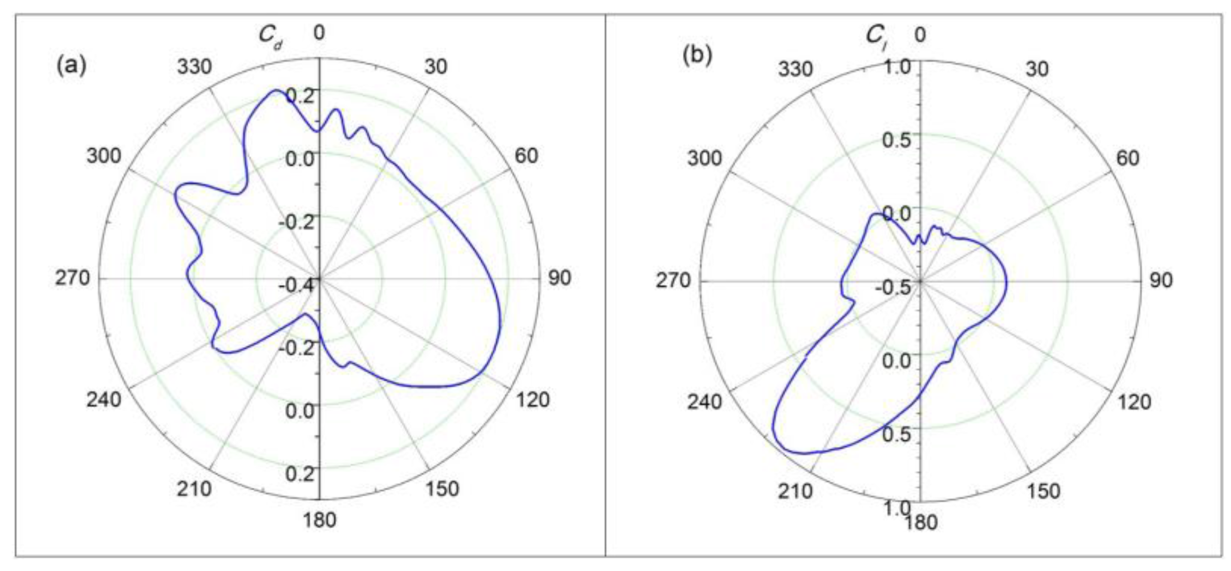
We note that Figure 21 predicts positive and negative values of C_d and C_l depending on the blade position of the crossflow runner. This behavior can be better observed through the polar graph shown in Figure 22 that represents the values of C_d and C_l corresponding to one blade (data from 7 s to 7.2 s). We discuss the results of Figure 22 with the aid of the velocity vectors and pressure contours at the simulated plane at t = 8.334 s (see Figure 23). The geometrical position of this case is similar to that of the 9.13 s case in Figure 19 since the flow pattern near the blades of the crossflow runner does not substantially vary in time (see Figure 19).

Figure 23 is used for explaining the performance of one single blade of the crossflow runner as it rotates (Figure 22). A blade of the crossflow runner generates an intense lift in the region 180° < θ < 240° (Figure 22) that corresponds to the zone where its orientation is more favorable for producing this aerodynamic force (see Figure 23). The existence of this zone was already observed in the analysis of VAWT (anticlockwise rotation; Figure 16). The main differences are that, under clockwise rotation, the inner vortex: (1) is less intense; and (2) has a center closer to the exit of the lower right upstream blades (verified by comparing cases with equal U and N but with different sense of rotation).

In comparison with the regimes studied in the VAWT section, the forced clockwise rotation modifies the triangles of velocities at both blade inlet and outlet points, leading to greater outflow velocities at the extrados of the lower left downstream blades. This implies higher pressure differences between the upper and the lower sides of the blades and therefore higher lift values. In addition, the pattern of the static pressure surrounding the entire crossflow runner seen in Figure 23 resembles that of clockwise rotating cylinders with a net pressure differences producing a positive lift (Magnus force). The position of the blade with the greatest contribution to drag is 60° < θ < 150° that corresponds to a zone with almost a perpendicular hit with the incoming flow (Figure 23).

On the other hand, the lift coefficient C_l for the entire runner shows a steady increase with N or, equivalently, with α (see Figure 24, in which, for completeness, data corresponding to Section 5 are included). For comparison purposes, C_l values corresponding to rotating cylinders are taken into account. The theoretical value for a plain rotating cylinder applies the Kutta–Joukowski theorem (see, e.g., [37]), being

$$C_l=\frac{\Gamma }{U},$$

(7)

where Г = 2πrω is the circulation, with r the radius of the cylinder and ω its angular velocity. Thus, the dotted line in Figure 24 has a slope equal to 2π whilst the shaded region includes measured and simulated data of C_l for cylinders in the range of 6 < U < 22 m s⁻¹ and 0 < N < 3000 rpm [38,39]. In Figure 24, the crossflow runner provides higher lift coefficients than those of cylinders (with and without spirals) at very low free stream velocities.

However, the relevant parameter for determining the performance of lift-based wind turbines is the drag C_d to lift C_l ratio rather than the lift coefficient C_l only. For this type of turbine, results indicate a dependence of C_d/C_l on 10^α valid for U ≤ 10 m s⁻¹ (see Figure 25). Simulations are limited to α values less than 0.8 since greater figures are achieved with unrealistic very high spinning velocities of the crossflow runner. Values of C_d/C_l for crossflow runners are as low as those recently obtained in state-of-the-art circulating airfoils (although the latter can be applied to a larger range of α). Overall, the C_d/C_l ratio for crossflow turbines is on the order of 10 times smaller than that of circulating cylinders at the same value of α.

According to the flow process diagram (Figure 2), an analytical approximation is applied for estimating the C_p value of crossflow HAWT. At spinning ratios α higher than 0.3, the flow at the wake of a crossflow runner clearly resembles that of a spinning cylinder at similar Re (see Figure 26; [39]). Therefore, the C_p equation is based on the analytical formulation developed by Sedaghat [15], who studied the performance of Magnus wind turbines (HAWT with spinning cylinders).

The analytical approximation applies the blade element-momentum theory in which the blade is divided into elements of infinitesimal thickness dr along the radial direction. The local equations of a blade element located at an arbitrary distance r take into account the value of the relative wind incidence angle, which changes with r. The power coefficient C_p is obtained after integrating a local power coefficient term from hub to tip radius (see [15] for details), being

$$C_p=8a\left(1-a\right){\lambda }_R{\int }_{{\mu }_0}^1\left[{\mu }^2+\frac{a\left(1-a\right)}{{\lambda }_R^2}\right]\frac{\left(1-\epsilon tan\beta \right)}{\left(\epsilon +tan\beta \right)}d\mu ,$$

(8)

where

$$\mu =\frac{r}{R};{\lambda }_r=\frac{\Omega r}{U};\epsilon =\frac{C_d}{C_l};tan\beta =\frac{{\lambda }_r\left(1+a^{\prime }\right)-\alpha /2}{1-a},$$

(9)

with r the radial distance from the center of the hub (of radius r₀) that rotates at $\Omega$, and R the radius of the turbine. In Equation (8), the axial flow induction factor a = 1/3 and the angular induction factor a’ follows

$$a^{\prime }=\frac{a\left(1-a\right)}{{\lambda }_r^2}+\frac{\alpha }{2{\lambda }_r}$$

(10)

Equation (8) is an integration from r = r₀ (µ = µ₀) to r = R (µ = 1) of the local contribution to C_p by taking into account the changes along the radial direction of the relative wind velocity with respect to the crossflow runner. Once µ₀ is kept fixed, Equation (8) depends only on the global spin ratio of the crossflow runner $\alpha$ and on the TSR (= ${\lambda }_R$) of the turbine. The drag to lift ratio ε used in Equation (8) is obtained after adjusting the data of Figure 25, giving

$$\mathsf{\epsilon }=\frac{C_d}{C_l}=0.863e^{-2.292{\alpha }_w},$$

(11)

with an R-square equal to 0.981.

In Equation (11), $\alpha$ is substituted by the local spin ratio ${\alpha }_W$ defined as

$${\alpha }_W=\frac{\omega D/2}{W},$$

(12)

with W the relative velocity of the air with respect to the blade. Thus, Equations (8) and (11) take into account that, for fixed values of TSR and global spin ratio $\alpha$, the resultant velocity over the crossflow runner varies along the radial distance r from the center of the hub, being

$$W=U\left(1-a\right){\left(1+{tan}^2\beta \right)}^{1/2},$$

(13)

and thus,

$${\alpha }_W=\alpha \frac{1}{\left(1-a\right){\left(1+{tan}^2\beta \right)}^{1/2}}.$$

(14)

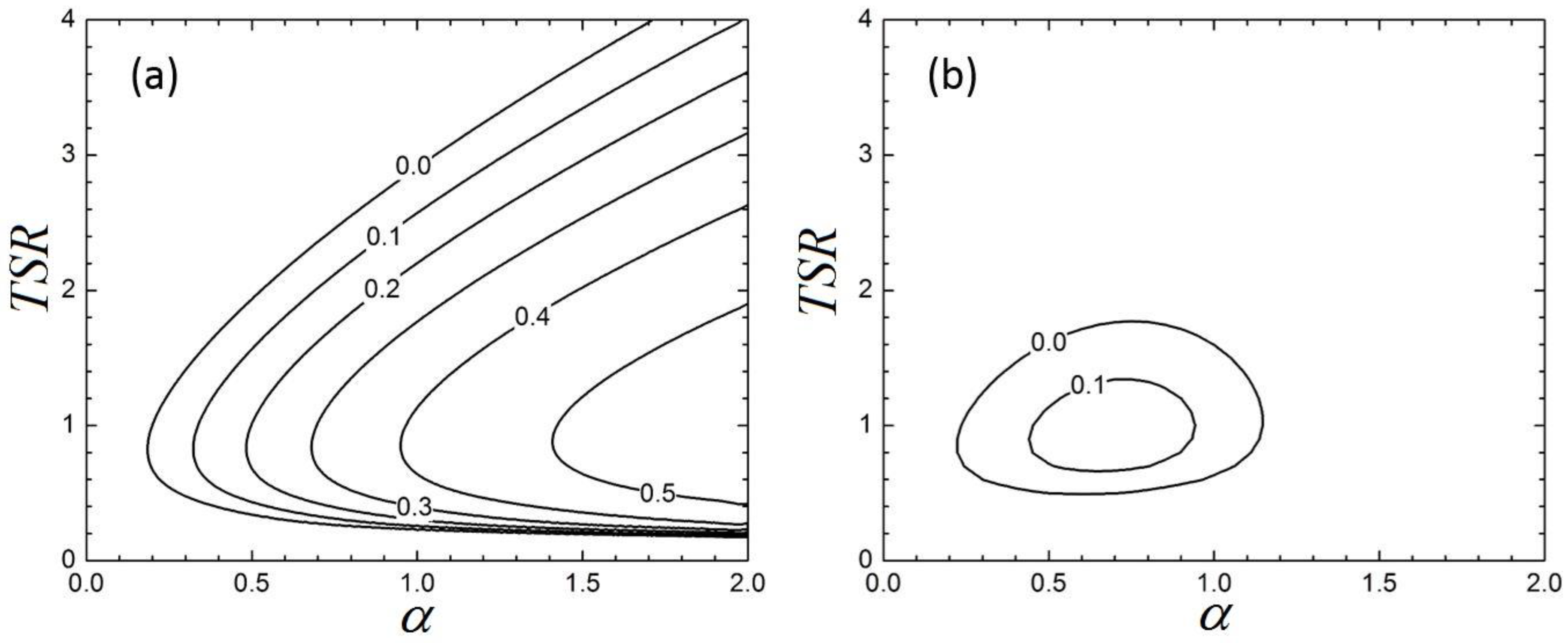
For µ₀ = 0.05, the power coefficient as a function of $\alpha$ and TSR is shown in Figure 27 where Equation (11) is assumed to be valid up to ${\alpha }_W$ ≈ 2. From Figure 25, this means a drag to lift ratio for a crossflow runner similar to that from circulating airfoils. Results indicate that the optimum TSR for HAWT is ≈0.8 for any spin ratio. At $\alpha$ = 1, C_p = 0.41, which represents an increase of 18% with respect to the performance of Magnus type HAWT (Table 1). For example, we estimate that a small HAWT with crossflow runners of diameter D = 0.062 m and length ≈ 1 m should spin at ω = 64.5 rad s⁻¹ and rotate with respect to the hub at Ω = 1.6 rad s⁻¹ for having a C_p = 0.41 when U = 2 m s⁻¹.

The required external power P_r for spinning the crossflow runners in HAWT is estimated by assuming that the required torque balances the resistant one generated by the flow over the entire runner. Thus,

$$P_r=\omega \int dM=\omega {\int }_{r_0}^R{C}_m\frac{1}{2}\rho W^2\frac{D^2}{2}dr,$$

(15)

where the last equality in Equation (15) considers the definition of the torque coefficient in Equation (5) and, as discussed previously, it uses the resultant relative velocity over the blade W.

From Equations (2), (9), (13) and (15), we define the required power coefficient $C_{pr}$ as

$$C_{pr}=\frac{P_r}{P_U}=\sigma \alpha {\left(1-a\right)}^2{\int }_{{\mu }_0}^1{C}_m\left(1+{tan}^2\beta \right)d\mu ,$$

(16)

where P_U is the power of the incoming flow in a surface area swept by the turbine and σ the turbine solidity defined as

$$P_U=\frac{1}{2}\rho U^3\pi R^2;\sigma =\frac{BDR}{\pi R^2},$$

(17)

with B the number of crossflow runners (i.e., of blades).

From the above, the available net power is P_net = P − P_r, from which the net power coefficient C_pnet is defined as

$$C_{pnet}=\frac{P-P_r}{P_U}=C_p-C_{pr}$$

(18)

Equation (18) depends only on the tip speed ratio TSR, the spin ratio of the runners α and the turbine solidity σ. The number of blades B in the blade element-momentum theory developed by Sedaghat [15] does not directly affect the global power coefficient, although it is taken into account in the calculation of the global torque. However, B indirectly affects the value of the net power coefficient since it modifies the turbine solidity value (an increase in B reduces C_pnet). Nevertheless, the effect of varying the number of blades on the performance of the HAWT would require complex 3D CFD simulations.

The C_m value in Equation (16) is estimated by fitting the simulated torque data against the local spin ratio for the U = 2 m s⁻¹ case, being $C_m=3.312{\alpha }_W^2+2.387{\alpha }_W+0.925$, with an R-square equal to 0.995. We do not expect substantial changes of C_m for other velocities, as inferred from Figure 17. Results of C_pnet for a solidity σ = 0.04 are also shown in Figure 27. In comparison with the C_p value, the available net power drastically reduces and makes unfeasible the applications of HAWT at high α due to the high demand of power for spinning the runners.

7. Conclusions

The potential use of crossflow runners as a single rotor in VAWT and as blades in HAWT has been numerically investigated. The 2D CFD model (ANSYS-Fluent) has been validated with experimental data obtained in a wind tunnel under runaway conditions. All cases have been simulated using the same domain as the one used in the experimental set up, so small variations in the results may occur when working in an open environment.

The working mode of crossflow runners in VAWT has a sense of rotation opposed to those runners used in HAWT. In VAWT, the crossflow runner rotates in the same direction than in the free case (autorotation or runaway regime). All working modes show that crossflow runners combine both drag-driven (upstream blades) and lift-driven (downstream blades) mechanisms for generating forces and torque, being the lift effect the most important factor in all cases. An inner vortex within the crossflow runner is formed, being more relevant when working in VAWT regimes than in HAWT ones.

The power coefficient C_p in VAWT is maximum at very low values of TSR (≈0.3), varying from 0.19 (our work) to 0.45 [9]. The discrepancy comes from working with different blade shapes, aspect ratios and Reynolds numbers (2.1 × 10⁴ here and 1.3 × 10⁵ in [9]). In general, high solidity runners are preferred for working in VAWT.

Crossflow runners used as blades in HAWT require an external (non-wind) power supply for spinning the runners at a fixed turning velocity. Drag, lift and torque coefficients over the whole runner for a 2D simulation show an oscillatory behavior with a dominant frequency that does not coincide neither with the runner spin frequency nor with the runner’s blade-to-blade one. This dominant frequency has its origin in the non-alternating vortex shedding detected downstream the runner and, because of its amplitude, it should be taken into account for avoiding resonances when designing the structural system of the turbine. This effect is not clearly observed when working in the VAWT mode.

The drag to lift ratio of runners for HAWT is comparable to that of circulating airfoils and ~10 times lower than that for cylinders at the same spinning ratios α. This leads to values of C_p of a HAWT obtained by applying an analytical approximation 18% higher than those expected in Magnus type wind turbines (i.e., C_p = 0.41 for TSR = 0.7 and α = 1). However, the available net power (extracted minus required for spinning the cylinders) is much lower, with a maximum net power coefficient C_pnet = 0.14 for TSR = 0.9 and α = 0.7. Thus, for HAWT applications, it is essential to design crossflow runners with aerodynamic blades to have very low drag to lift ratios and, at the same time, low resistant torques.