Exergo-Economic Evaluation of the Cost for Solar Thermal Depuration of Water

Abstract

A detailed assessment of the cumulative cost of clean water production by a natural circulation solar thermal system is presented. The system is designed and sized for sufficient residence time for pasteurisation, in a buoyancy-driven self-compensating circuit. Since it does not consume electricity, it is suitable for developing countries or emergency locations with safe drinking water issues. The principles for design and off-design simulations are explained and discussed. The simulations were performed for seven different locations, representing variable climate conditions in selected regions where there is an evident need for safe water. The results include an exergy and exergo-economic analysis. The production capacity reaches typically from 0.04 to 0.1 m³/day per m² of solar collector depending on the location. The annual cost of water production ranges between 2.2 and 6.8 €/m³ making the proposed system fairly competitive; the energy- and price-performance of the system is compared to a reverse osmosis/photovoltaic system, representing a high-tech alternative for the purpose of water purification.

1. Introduction

Migrations, peace and development are some of the most important problems that the global society has to solve in the future, but there are many discussions about how we can do that: these arguments have been analysed by many organizations and the World Economic Forum (WEC) [1] is one of the most important.

According to the WEC meeting report, water crises are considered as one of the main problems in the world, since the migration of millions of people is involved, with relevant issues in terms of health and possible deaths. Indeed, renewable water per capita availability (the part of water that can be used by humans and can be re-integrated by the hydrologic cycle) has been decreasing since 1970. According to this report, the problem is strictly linked with the availability of energy resources.

Industrial countries are trying to solve this problem using high technologies solutions for water treatment and disinfection, for example ultrafiltration and reverse osmosis (RO), and multi-flash systems that bring water to evaporation and condensation. RO is a process based on pumping water across a non-porous membrane which intercepts monovalent ions such as Na⁺ and Cl⁻. RO is effective on several contaminants, from hydrocarbons to heavy metals and bacteria but there are many problems due to biofouling of membranes and to the integrity loss after chemical attacks (for example by NH₃). Indeed, the membranes and the raw water need many pre-treatments such as disinfection (in this light, integration of pasteurization and RO can be recommended). Another problem in RO is the disposal of the material (called the concentrate) separated from the treated water by the membrane, that must comply with local regulations and may cause relevant environmental impacts; but the main problem is the large need of energy, electricity and high-pressure pumps that makes RO very expensive [2].

Developing countries are not able to use these technologies on a wide scale, because of economic and technical reasons: in many regions of the world, the electrical grid is not available, and sun is the only source of energy.

This is why simple systems like SODIS [3] were proposed: SODIS applies solar disinfection utilizing used, low-cost plastic bottles, taking advantage of sterilization due to the UV content of the solar radiation which destroys the cellular membrane of bacteria; on the other hand, pathogens inside bottle die because of high temperatures reached by the water. SODIS is a simple and effective process focused on the re-use of materials (PET and PVC bottles), characterised by an extremely low level of technology; however, it needs careful application and individual training. This method has gathered interest and to prove it viable many enhancement investigations were performed.

Another technology, being halfway between above mentioned systems in terms of technology level is solar pasteurization utilizing solar thermal collectors and inexpensive piping/vessel technologies. It is assumed that such a system will be a proper solution for mid- or long-term clean water scarcity problems resulting from natural disasters or social emergencies, while short-term emergencies are usually dealt with more expensive packaged units. The paper covers energy, exergy and exergo-economic analysis of a computationally designed natural circulation solar thermal pasteurisation system. The simulations of annual operation were performed for seven locations which are, or could be, affected by lasting emergencies with access to potable water becoming a survival matter. The aim is to calculate the cumulative cost of clean water production in these regions and to compare it with cost of water produced by a high-tech, photovoltaic-driven RO system. According to the statement of Ranjan and Kaushik [4], only a limited number of research papers in the topic of exergy analysis of solar distillation system are avialable. As will furtherly result from the literature review in Section 1.1, the investigation in this paper is expected to fill the gaps in the research field of a natural circulation buoyancy-driven solar thermal water depuration system.

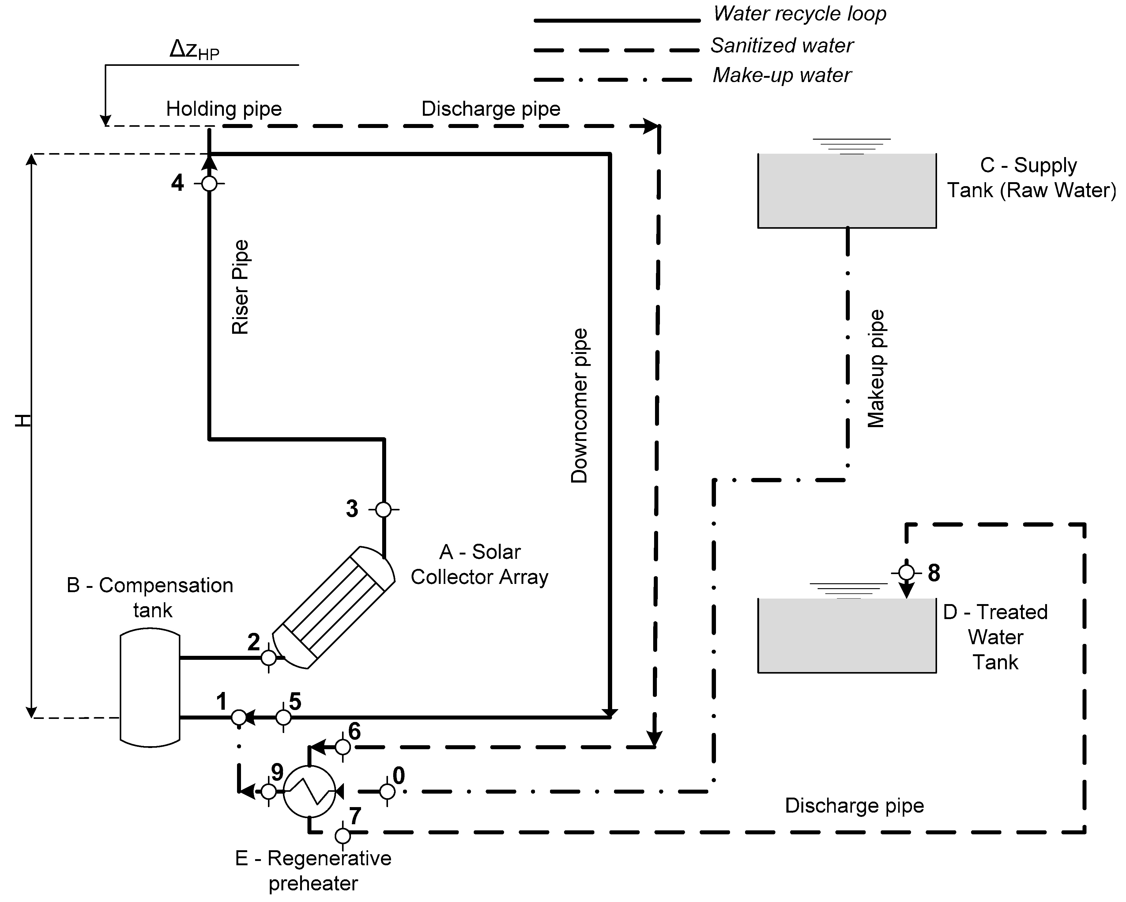
1.1. Pasteurization of Water with Solar Collectors in Recirculation System—Existing Research and Investigated Plant

Pasteurization is a process named after Louis Pasteur, an eminent researcher of the 19th century; the process aims to kill all the pathogens present in water, by applying and maintaining an adequate temperature for a definite time [5].

These temperature levels can be easily obtained using flat-plate solar thermal collectors because the closed-circuit process does not involve significant evaporation losses of water; reaching and maintaining the required temperature can be guaranteed by devices such as a thermostatic valve or a recirculation arrangement. A thermostatic valve can control the flow rate guaranteeing that the processed water remains for sufficient time at high temperature. Many experiments of this technology can be found in the literature: for example Anderson [5] used a parabolic solar thermal concentrator to pasteurize water using a valve to control the set point temperature at 75 °C and thus treat 0.089 m³/(h·m²) of water. As reported in [6], Jorgensen and Stevens managed to treat, at the set point temperature, 0.055 m³/(h·m²) of water using flat plate collectors after a significant warm up period and the Safe Water System company (Honolulu, HI, USA) produced in 2002 one of these systems which can produce 0.202 m³/(h·m²). Carielo da Silva et al. [7] performed tests on a solar pasteurizer based on the use of flat-plate solar collector with flow control valves, setting various outlet temperature levels (55–85 °C) and residence times (3600-15 s, respectively). During the tests, the pasteurizer was able to produce daily up to 0.03 m³ of clean water.

El Ghetany et al. [8] shared their results on numerical simulation and experimental validation of a solar water disinfection system, where the outlet flow temperature is controlled by a solenoid valve. Numerical modelling is also applied by Abraham et al. in [9] to examine a system including a parabolic trough collector, a thermally activated valve and a fluid-to-fluid heat exchanger, able to inactivate water pathogens. The study presented by Gill et al. in [10], presents experimental results for an existing continuous flow disinfection system, where a valve controlling flow rate is applied with compound parabolic concentrators.

Even though these systems are simple and easy to build, the thermostatic valve depends on electricity, which is not available in some parts of the world (it can be provided by an off-grid PV system); furthermore, they can have several problems, especially when the radiation decreases and the collector operates under stagnation conditions: under these conditions, the flow is stopped and the system becomes completely inefficient. The thermostatic valve, as every electronic device, is also subject to failures, especially when operating on water resources with high salt contents.

Because of these difficulties, a buoyancy-driven system was built and tested by Duff and Hodgson [6]. The model discussed in this paper was developed from this original idea, but the operation scheme has been revised and modified, as shown in Figure 1.

In the proposed system [11], raw water flows from the supply tank (C) to the treated water tank (D) with no use of electricity: the driving force is provided by the variation of water density due to its heating in the solar collector (A). A set-point temperature of water is defined and fixed to 85 °C: in these conditions, following [12] we assume that disinfection can take place in few seconds, so that the residence time inside the circuit is always adequate. The water is heated inside the solar collectors and it flows through the “Riser pipe”; if its temperature is below 85 °C, the system operates in a closed recirculation loop and the “Downcomer pipe” brings back the water to the solar collector; the circuit is run under this configuration until water reaches the set-point temperature.

When the set point temperature value (85 °C in the present case) is reached, the thermal expansion due to water heating inside the collector determines spill-over of the flow; the spill-over flow rate is collected by the “Discharge pipe”. The system configuration is changed from closed to open, with a closed-loop recirculating circuit and two inlet/outlet pipe sections (make-up and discharge pipes; dotted lines in Figure 1).

The spill-over volume is automatically (i.e., by gravity) replaced by the same volume of raw water (supplied by reservoir C) inside the circuit and it flows to the treated water tank; the inlet flow rate is pre-heated in a regenerative heat exchanger E (which also cools down the flow rate directed to the treated water tank), and it is mixed with the remaining hot water inside the circuit.

Adoption of an insulated compensation tank (B) is suggested with respect to the original scheme proposed in [6], in order to increase the mass of water inside the circuit: in this way, the treated water flow is increased, as well as the inlet flow of raw water. Water evaporation is prevented by the closed circuit (the two tanks C and D contain water close to ambient temperature), and scaling problems are consequently limited also considering the flexible sizing of the piping necessary for natural circulation.

This process is designed to provide the disinfection of water in a very simple, cheap way so that it can be applied in isolated places. It only uses solar energy, and a simple preliminary sand-filtration of the raw water should allow to avoid problems of obstruction of pipes.

In the following, a thermo-fluid dynamic model of the proposed natural circulation pasteurisation system is described. After application to design, the same model is adapted to include climatic variables and examine different locations on an annual operation time. Fundamental guidelines for sizing and off-design simulation of the cycle are presented. An exergy analysis was performed so that an exergo-economic evaluation of the cost for solar thermal depuration of water was finally possible. The water production costs are confronted with a high-technology solution.

2. Methodology

2.1. Design and Off-Design Simulation; Energy Analysis of the System

2.1.1. Sizing the Natural Circulation Pasteurisation System

The system is assembled from a basic set of components: solar collectors, pipes, a compensation tank, two tanks to store raw and treated water and a regenerative heat exchanger.

A commercially available flat plate solar collector is considered [13], its modelling is based on the typical 2nd order Bliss Equation (1):

$${\eta }_{SC}=C_0-C_1\frac{\Delta T_m}{G}-C_2\frac{\Delta T_m{}^2}{G}$$

(1)

where C₀, C₁, C₂ are provided by the constructor of the collector and $\Delta T_m$ is a temperature difference between water in the solar collector and ambient, as visible in Equation (2):

$$\Delta T_m=T_{av\_23}-T_{amb}$$

(2)

The sizing is determined by a set of three governing Equations (3)–(5):

$$\dot{m}{C}_P\left(T_3-T_2\right)={\eta }_{SC}G{A}_{SC}$$

(3)

$$\Delta P=gH\left({\rho }_2-{\rho }_3\right)$$

(4)

$$\Delta P=k{\dot{m}}^2$$

(5)

Equation (3) describes the heat balance of the fluid flowing across the solar collectors; Equation (4) represents the buoyancy-induced pressure driving force, with $H=z_2-z_3$ representing here a design variable, connected to the circuit length L which is a multiple of H. Equation (5) represents the resistance of the pipes which determines the pressure losses contrasting the driving force as the flow conditions are turbulent (the Reynolds number assumes values > 2000, typically between 3000 and 16,000). Constant k is the circuit equivalent flow constant, accounting for the sum of concentrated and distributed losses (these last depending on pipe length, diameter and roughness).

The spill-over conditions are reached when water is warmed to 85 °C—a temperature level ensuring safe pasteurization in a few seconds. Pasteurized water will then flow over the top of the holding pipe due to its volume increase induced by the density change. The initial reference water density conditions (circuit filling) are defined for 20 °C. The variation of volume in spill-over conditions can be obtained applying set-point conditions to Equation (6):

$$\Delta V_{85°}=m\left(\frac{1}{{\rho }_{85°}}-\frac{1}{{\rho }_{20°}}\right)$$

(6)

Assuming the diameter of the holding pipe, we can find its length using Equation (7):

$$\Delta z_{HP}=\Delta z_{85°}=\frac{\Delta V_{85°}}{A_{HP}}=\frac{m}{A_{HP}}\left(\frac{1}{{\rho }_{85°}}-\frac{1}{{\rho }_{20°}}\right)$$

(7)

Using the parameters set in

Table 1. System parameters—Design.

System Parameters
C0	0.78	C1	1.75 W/(m2·K)	C2	0.00625 W/(m2·K2)
Tamb	30°C	G	1000 W/m2	ASC	2·1.95 m2
L/H	5.3	H	1.5 m	DHP	0.15 m

, the previous system (3)–(5) can be traced back to a three variables system ($\dot{m}$, D and k) with one only solution.

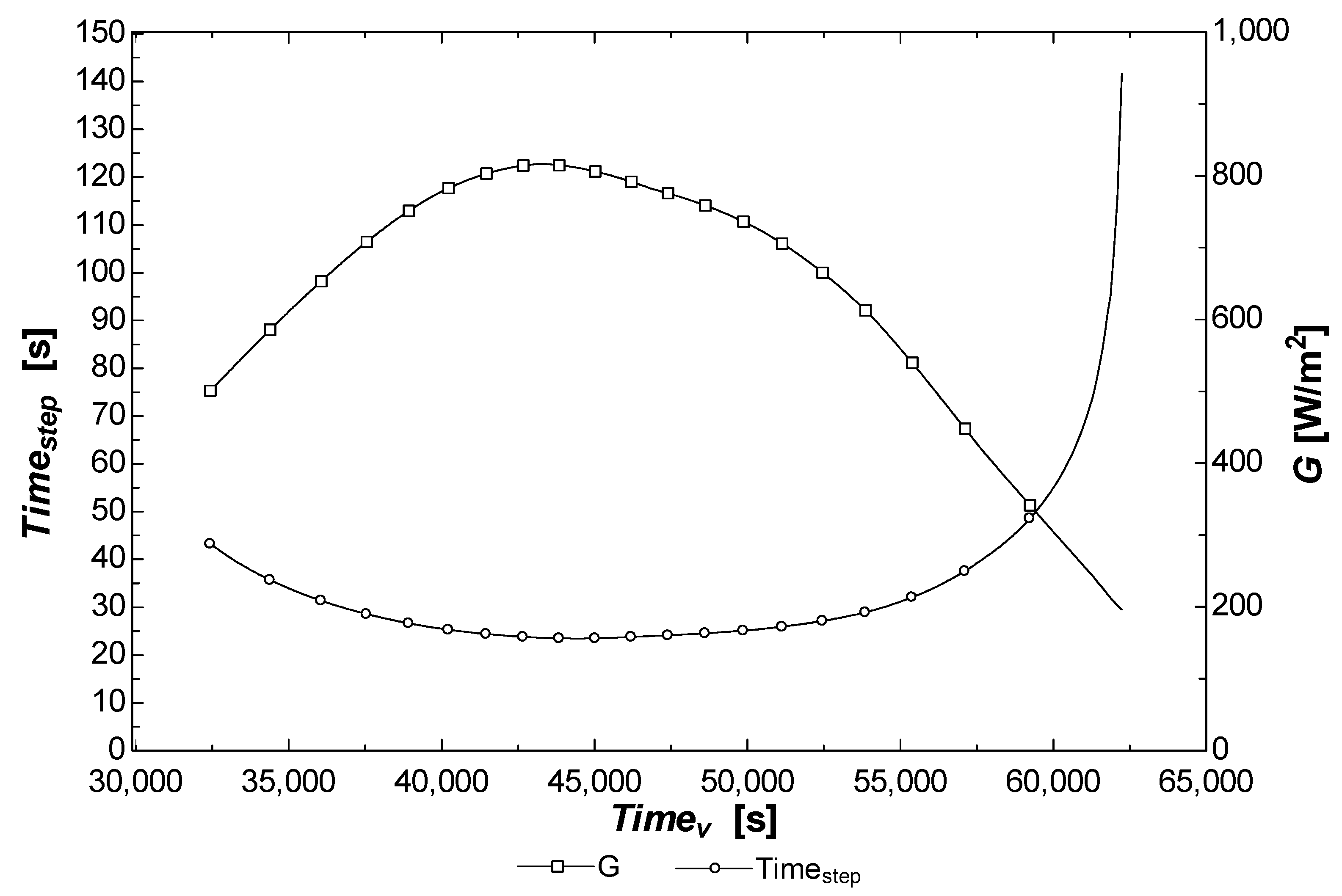
2.1.2. Off-Design Simulation of the System

After having sized the system for the design conditions, analysing its performance under off-design conditions is very important. The simulation model is based on the same equations used for sizing; the geometry of the system being now fixed, the main output variable is the flowrate $\dot{m}$, G and T_amb are time-dependent input variables.

In time-forward simulations a time discretization is necessary; in this case an evolutionary variable time step is physically determined as the time needed to complete one full loop (time needed by the whole volume of water to pass all of the pipes):

$${\tau }_i=\frac{L}{V_{av,i}}$$

(8)

This time-marching approach based on a physical, adapting time step is a specific feature of the present study and represents a fundamental innovation with respect to other dynamic simulators working with fixed time steps.

In the dynamic off-design model, the values of k, D are known from the system sizing; the design value of mass flow rate $\dot{m}$ (in equations denoted as ${\dot{m}}_{gg}$) is only used as starting guess value of the mass flow rate, but the real value is obtained using an iterative calculation process.

First, another value is obtained by the natural circulation Equation (9) resulting from Equations (4) and (5):

$${\dot{m}}_g=\sqrt{\frac{gH\left({\rho }_2-{\rho }_3\right)}{k}}$$

(9)

where ${\rho }_2$ and ${\rho }_3$ are calculated before using guess value ${\dot{m}}_{gg}$.

Then the deviation is calculated using Equation (10):

$$dm=\left|\frac{{\dot{m}}_{gg}-{\dot{m}}_g}{{\dot{m}}_g}\right|$$

(10)

If $dm>0.001$ a new guess value must be produced; to do that, a 75% under-relaxation value was applied to improve the stability of the method, as indicated in Equation (11):

$${\dot{m}}_g=0.75{\dot{m}}_{gg}+0.25{\dot{m}}_g$$

(11)

When $dm<0.001$ the method reaches convergence and the new calculated value of $\dot{m}$ in this step can be used as a guess for the following one.

Using an estimate of thermal losses in each branch, the temperature in each node of the circuit is evaluated, so that it is possible to find the value of the fluid volume variation at every time step i with the reference to the starting (circuit-filling) conditions following Equation (12) and the thermal dilatation across the holding pipe as in Equation (13):

$$\Delta V_i=m\left(\frac{1}{{\rho }_i}-\frac{1}{{\rho }_{20°}}\right)$$

(12)

$$\Delta z_i=\frac{\Delta V_i}{A_{HP}}=\frac{m}{A_{HP}}\left(\frac{1}{{\rho }_i}-\frac{1}{{\rho }_{20°}}\right)$$

(13)

The balance of the regenerative heat exchanger (RHE) is formally given by Equation (14):

$${\dot{m}}_{MU}{c}_p\left(T_9-T_0\right)={\dot{m}}_{MU}{c}_p\left(T_6-T_7\right)$$

(14)

As a result, at exit of the RHE the treated water is stored close to ambient temperature (T₇), making it immediately available for drinking and other valuable uses; while the inlet raw water (${\dot{m}}_{MU}$) is effectively pre-heated and produces thus a moderate cooling of the recirculating water (${\dot{m}}_{Ric}$) according to the following mixing energy balance (15). The balance calculates the temperature T₁ of water leaving the mixer. T₁ is calculated using conditions from the previous time-step, since the mixer is here the component closing the recirculation loop:

$$T_1={\frac{{\dot{m}}_{Ric}{T}_5+{\dot{m}}_{MU}{T}_9}{{\dot{m}}_{Ric}+{\dot{m}}_{MU}}|}_{step-1}$$

(15)

The analysis here presented allows calculation of the amount of the clean water produced in a defined time-period with reference to the installed solar collector surface area. It also provides information on the amount of solar heat required to purify a unit of water.

The off-design simulations provide a performance estimate of the system operating for one standard year in seven various locations: Manila (Philippines), Aden (Yemen), Johannesburg (South Africa), Nairobi (Nigeria), Larnaca (Cyprus); Pantelleria and Brindisi (Italy). The sites were deliberately chosen as cities representing regions with existing or potential water sanitation problems, characterized by variable climate conditions. Brindisi could be treated as an exception with the lowest clean water access problem potential; it was however included for the comparison purposes.

2.2. Exergy Analysis

Energy analysis itself does not provide information about internal process inefficiencies. An exergy analysis of the system may help to understand the main sources of exergy destructions or losses, and enables further interpretation of the seasonal productivity for different locations. It is true that the exergy value of depurated water is low (as that of the original raw water); however, in the depuration process larger temperatures (and exergies) are involved, so that a process analysis of exergy destructions and losses can be anyway recommended. Moreover, exergy analysis is a substantial step for the exergo-economic evaluation of the cost of purified water produced by the system [14].

In the analysed case, the exergy of the fluid is calculated for every point of the circuit. Additionally, the friction losses for each pipe branch were accounted in terms of friction pressure loss.

Exergy is generally defined as the maximum work obtainable from a system or a process through an interaction with the surrounding environment. A characteristic formula for the exergy of the substance is defined after [14,15] and given in Equation (16):

$${\dot{Ex}}_j={\dot{m}}_j\left[\left(h_j-h_o\right)-T_o\left(s_j-s_o\right)\right]$$

(16)

In direct terms, the exergy efficiency is defined as ratio of output and input exergy. The indirect definition of exergy efficiency takes into account the exergy destructions and losses which influence the irreversibility of the system operation. An exergy destruction derives from friction or irreversibility of heat transfer within a defined control volume, while an exergy loss is assigned to exergy transfer to the surroundings. Hence, the exergy efficiency is pictured with Equation (17):

$${\eta }_x=\frac{{\dot{Ex}}_{out}}{{\dot{Ex}}_{in}}=1-\frac{{\displaystyle \sum }{\dot{Ex}}_D+{\displaystyle \sum }{\dot{Ex}}_L}{{\dot{Ex}}_{in}}$$

(17)

The exergy analysis rests on recognition of losses and destructions within the system. In the present case, the following contributions can be identified:

• Solar collector exergy loss—assuming that radiation is available at infinite (or very high) temperature, it can be approximately taken as coincident with the collector ambient heat loss [16,17];
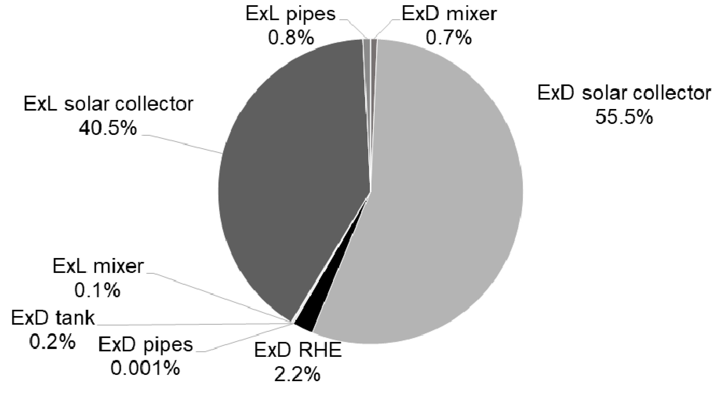
• Solar collector exergy destruction—resulting from the exergy balance of solar collector component; as energy transferred to the fluid is conserved, this destruction is essentially a heat transfer irreversibility;
• Piping insulation exergy loss—resulting from standard heat transfer models for thermally insulated pipe lines
• Piping friction exergy destruction—predicted using turbulent flow pipe correlations; entropy calculated from the overall pressure loss
• Regenerative heat exchanger exergy destruction (spill-over)
• Make-up mixing exergy destruction (spill-over)
• Piping insulation exergy loss (spill-over; make-up and discharge pipes)
• Piping friction exergy destruction (spill-over; make-up and discharge pipes)
• Compensation tank unsteady exergy destruction—this results from the model of the compensation tank as a dynamic-effect carrier; the tank is modelled as a fixed volume with variable temperature, internal energy, and closed-system exergy accumulation [18]. The transient exergy destruction rate ${\dot{Ex}}_{Dtank}$ associated with the compensation tank is a difference between exergy rate of water flowing into the tank and water leaving the tank at given time step and change of internal exergy of the tank during the whole time step.

2.3. Exergo-Economic Analysis

Exergy, as has been said, is not only a thermodynamic property of an energy carrier, but it can be defined as the maximum work obtainable from the carrier through an interaction with the surrounding environment. Exergy can be seen as the useful part of energy, and a user pays only for this part. Consequently, rather than energy, it is useful and rational assigning cost to the exergy. This is the principal characteristic of the exergo-economic analysis that combines exergy and economic analysis by introducing costs per unit of exergy [19]. This analysis, providing useful information not achievable with energy and economic analysis, can be used to analyse, plan and optimize the energy systems [14].

In this study, the exergo-economic analysis of the system was applied to calculate the specific cost of purified water production.

The approach outlined in [14,19] was applied to perform the exergo-economic analysis: for each component k a cost balance given as in Equation (18) is formulated:

$${\displaystyle \sum }_{out}{\dot{C}}_{out,k}+{\dot{C}}_{w,k}={\dot{C}}_{q,k}+{\displaystyle \sum }_{in}{\dot{C}}_{in,k}+{\dot{Z}}_k$$

(18)

$${\displaystyle \sum }_{out}{(c_{out}\dot{E}{x}_{out})}_k+c_{w,k}{\dot{W}}_k=c_{q,k}\dot{E}{x}_{q,k}+{\displaystyle \sum }_{in}{(c_{in}\dot{E}{x}_{in})}_k+{\dot{Z}}_k$$

(19)

Subsequently, for every component k with N_k numbers of exiting exergy streams, N_k−1 auxiliary equations were defined [14]. In this way a linear system of equations is formulated to calculate costs per unit of exergy in all the streams of the system.

The system under consideration is not an installation working always under design conditions, but the operating conditions vary continuously at each generic time step according to environmental data (overall radiation and ambient temperature). Moreover, the system can take two different configurations during the daily operation period: closed loop and spill-over, so the cost balances for each component are not directly applicable. Therefore, in this study, the sum of the exergy values at each time step during a daily operation period is calculated at each of the points of the circuit. Then these daily integral values of exergy are included in the cost balances. Therefore, the unit of time for exergo-economic balances does not correspond to a second but to a day considered as a certain number of operating hours that varies according to the location and month. As to clarify, the terms with daily operating time as the unit of time will be indicated with superscript “d” instead of the dot notation. Accordingly, also the term ${\dot{Z}}_k$ in the balances is calculated considering the daily operating time as the unit of time (so it becomes $Z_k^d$). In the calculations, the operating and maintenance costs are considered to be negligible because the system is very simple, cheap and of easy maintenance.

In particular, for each component, the annual investment cost is calculated with Equation (20) at first:

$$Z_k^{an}=\frac{ir{\left(1+ir\right)}^n}{{\left(1+ir\right)}^n-1}{Z}_k$$

(20)

where an interest rate of 9% and an operation period of 15 years are assumed.

Then the $Z_k^{an}$ value is divided by the amount of operating hours in a year and then multiplied by the daily number of operating hours, in order to obtain the $Z_k^d$ (€/day) value to be considered in the cost balance.

Two more important assumptions are made: the cost of exergy losses and the cost of raw water are set to zero. The term ${\dot{W}}_k$ (in Equation (19)) is zero for each component because of the characteristics of the system.

With these balances the cost rate (€/day) associated with the exergy of water exiting from the discharge pipe ($C_{out,dis\_pipe}^d$) is calculated. Then, dividing this value by the amount of purified water produced in a day ($m_{MU}^d$), a preliminary specific cost of treated water (€/kg) is found. Anyway this value does not take into account the annual investment cost of the overall system installation ($Z_{inst}^{an}$) and the contribution of the annual investment cost of makeup pipe ($Z_{mu\_pipe}^{an}$), treated water tank ($Z_{tr\_w\_tank}^{an}$), and supply tank ($Z_{sup\_tank}^{an}$). In fact these last three annual investment costs are associated with initial and terminal components so they cannot be considered directly in the cost balances. To calculate their contribution to the cost of purified water, the sum of these annual costs ($Z_{inst}^{an}$, $Z_{mu\_pipe}^{an}$, $Z_{tr\_w\_tank}^{an}$ and $Z_{sup\_tank}^{an}$) is divided by the amount of treated water produced in one year ($m_{MU}^{an}$). Then this result is added to the preliminarily calculated specific cost of purified water originating from cost balances. Consequently, the specific cost (€/kg) of treated water produced ($C{s}_{tr\_w}$) in a certain location and month is given by:

$$C{s}_{tr\_w}=\frac{C_{out,dis\_pipe}^d}{m_{MU}^d}+\frac{Z_{inst}^{an}+Z_{mu\_pipe}^{an}+Z_{tr\_w\_tank}^{an}+Z_{sup\_tank}^{an}}{m_{MU}^{an}}$$

(21)

In order to calculate the annual investment cost of the overall system installation, the total cost of installation should be considered instead of the purchase cost of component in Equation (20). The total cost of installation is assumed to be 20% of the total purchase cost of the system [14].

The purchase costs considered are costs of real components available on the market [20,21,22,23,24,25] except that of the solar collector that is calculated multiplying the surface area of the solar collector by the specific value of 227 €/m² that was found from the literature [26].

2.4. Tools

The sizing, off-design simulation and further exergy and exergo-economic evaluation of the proposed system were performed using two types of software: Engineering Equation Solver (EES) (version 9, F-chart software, Madison, WI, USA) [27] and Transient System Simulation Tool (TRNSYS) (version 17, Thermal Energy System Specialists, LLC, Madison, WI, USA) [28]. EES was the frame of the numerical model. While performing the heat transfer analysis it was possible to take advantage of the built-in heat transfer correlation library [29]. TRNSYS software and its Meteonorm libraries [30] helped retrieving the varying values of incoming solar radiation and ambient temperature. The data for the seven chosen locations were used. The simulations were performed once the whole-year weather data were processed to create average days statistically representative of specific months of the year. The hourly averaged data were imported into Lookup Tables of EES and then respectively interpolated.

3. Results

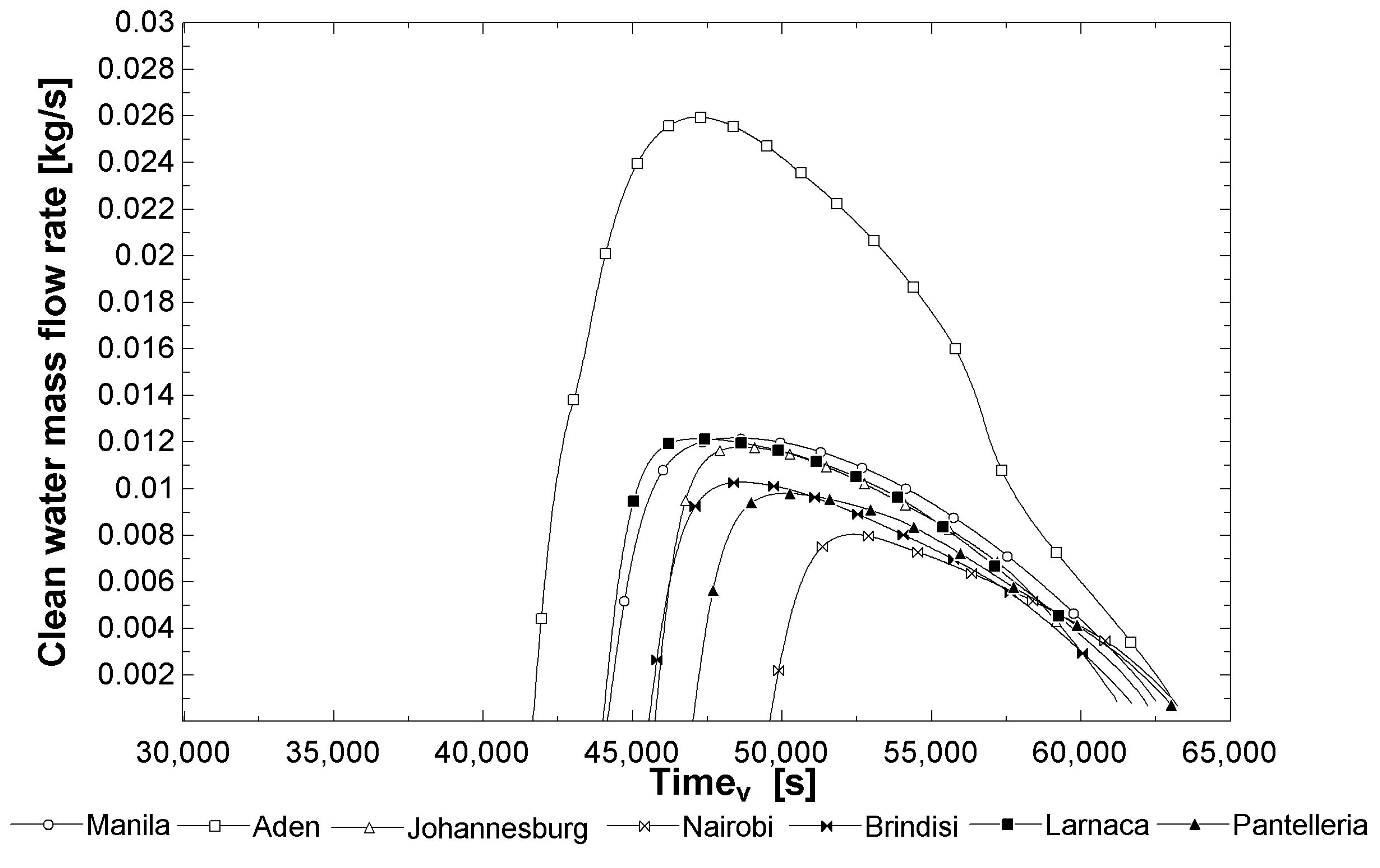
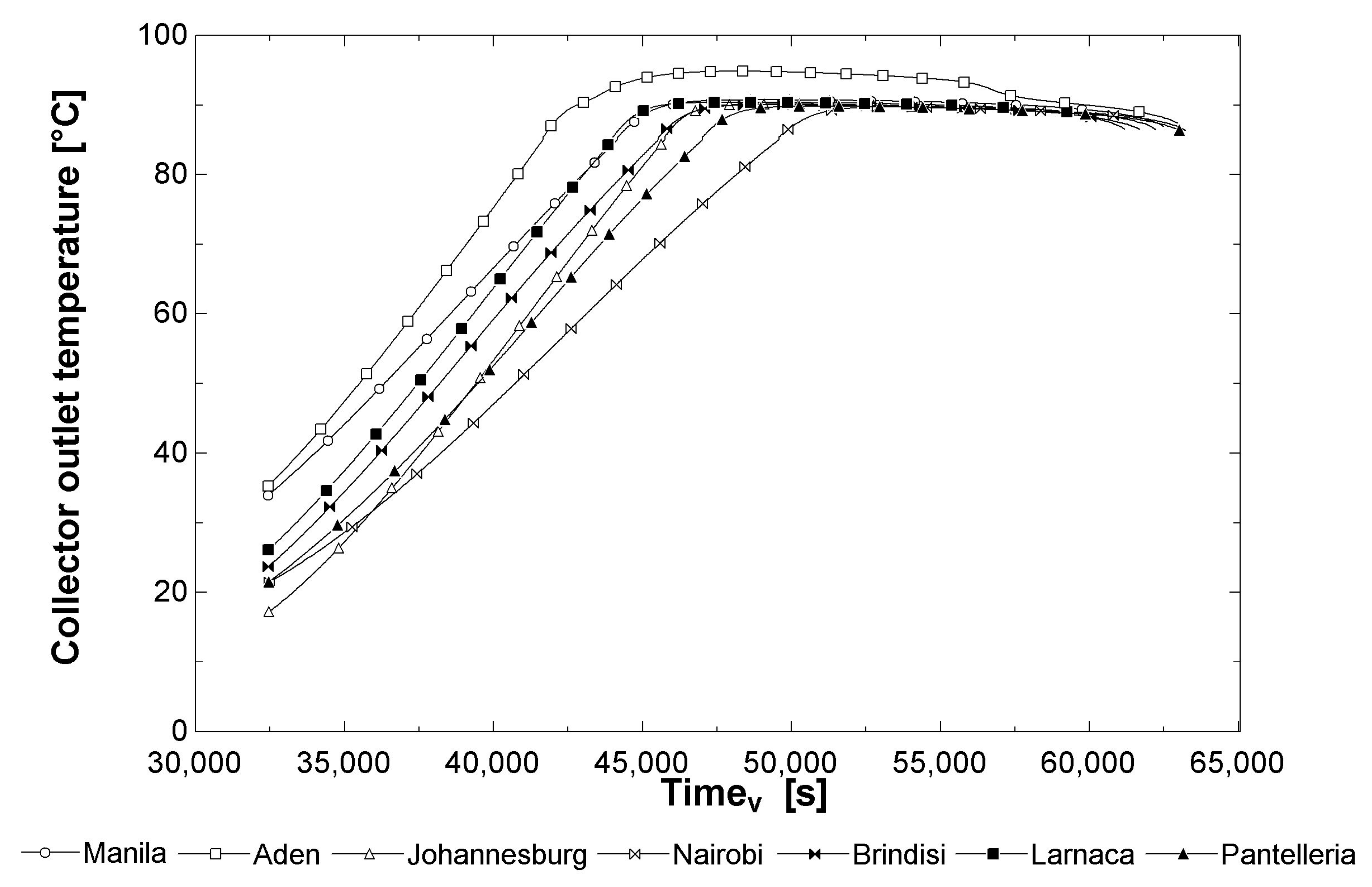
3.1. Results: Productivity (from Thermo-Fluid Off-Design Analysis)

The design sizing, using all the assumptions and equations in Section 2.1.1, allowed to calculate the output variables reported in

Table 2. Results of design sizing.

Design Sizing Results
D	0.02 m	L	8 m	$\dot{m}$	0.0255 kg/s
Δp	360 Pa	k	552,000	η	0.692
$z$	2.7 kW	AHP	0.785 cm2	ΔzHP	0.147 m

.

Following the methodology of simulation, the variable-adaptable time step was evaluated after Equation (8); a typical operation day time history (the representative day of May in Manila) is shown in Figure 2.

The main performance indicator is the mass flow rate of water production, presented in Figure 3 for an average day of May in all the seven locations examined.

The figure shows that the mass flow rate of clean water is strongly dependent by latitude. Indeed, in Aden, a location with a hot desert climate, the water production is distinctly higher than in other locations. The lowest production of clean water in May occurs in Nairobi; this can be explained by the fact that April and May correspond to the rainy season in this closest-to-equator location. Since Brindisi and Pantelleria belong to the same Mediterranean climate, the mass flow rate values are comparable, but sensibly lower in comparison with more tropical and sub-tropical places (Larnaca, Manila, Johannesburg).

The variation of mass flow rate during the average day of each month was calculated for every location considered; the typical output trend is similar to that presented in Figure 3.

Water production varies together with the radiation conditions during the day and during the year; the system is not productive during the main part of the morning when water warms up, the maximum of production corresponds to the peak of radiation; then it decreases until zero.

Another interesting parameter is the outlet temperature from the collector: Figure 4 shows that water warms up until it overflows, then the outlet temperature from the collector has a stabilization on a constant value over 85 °C. Evidently, the thermal output of the collector is able to maintain a constant temperature when the spill-over mode is activated. The observations on the outlet temperature variation during the day correspond to these made on mass flow rate distribution. A system located in the hot arid climate of Aden would be the first to achieve the pasteurisation temperature of 85 °C. High initial temperature resulting from high ambient temperature in the morning is also giving an advantage to the dynamics of temperature increase. However, the example of Johannesburg and the slope of its temperature curve indicates that if the solar radiation is high enough, the temperature may increase much faster than for the locations of high initial water temperature, but of lower irradiation.

Simulations revealed that the system is potentially able of a maximum daily productivity ranging between 40 and 102 kg per m² of solar collector, depending on the location. The tests of a density driven system with an internal convection loop proposed by Duff et al. [6] confirmed an even higher result—up to 200 kg/m² of clean water were reported in one day.

Table 3. Simulation results for all seven locations.

No	Location	Manila (Philippines)	Aden (Yemen)	Johannesburg (South Africa)	Nairobi (Kenya)	Brindisi (Italy)	Pantelleria (Italy)	Larnaca (Cyprus)
1	Coordinates	14.52° N 121°E	12.83° N 45.03° E	26.13° S 28.23° E	1.3° S 36.75° E	40.65° N 17.95° E	36.82° N 11.97° E	34.88° N 33.63° E
2	Annual solar radiation, MWh/(m2·year)	1.818	2.244	2.254	1.933	1.701	2.111	1.702
3	Annual productivity, m3	48.792	106.354	56.819	41.961	28.342	28.347	59.525
4	Solar collector: annual exergy destruction, MWh/(m2·year)	0.869	1.121	1.084	0.931	0.787	0.910	0.799
5	Solar collector: annual exergy loss, MWh/(m2·year)	0.626	0.739	0.777	0.677	0.584	0.642	0.617
6	Water production cost—Natural circulation, €/m3	4.64	2.24	4.19	5.20	6.80	6.77	4.01
7	Water production cost—ROPV, €/m3	5.34	4.02	3.81	5.13	5.96	6.87	4.83

collects synthetic results obtained for each location; the integral values of clean water production are reported in row number 4. The highest obtainable amount of clean water produced, 106 m³, was obtained in Aden (Yemen). Although the annual solar radiation value is almost the same in Johannesburg (South Africa), the yearly water production is much lower: 57 m³. This can be explained by the phenomenon of high temperature drop during the night in Johannesburg’s climatic zone. Because of that, a large amount of morning solar radiation is spent for raising the temperature of water in the installation up to the preset pasteurisation temperature. In this way, the clean water production in subtropical highland climate (Johannesburg) becomes similar to the potential output in the subtropical Mediterranean climate typical for Cyprus (Larnaca).

3.2. Results—Exergy Analysis

The output exergy of the natural circulation water depuration system is the exergy of purified water, while the input is the exergy of solar radiation which drives the whole process.

The exergy balance is verified at each generic time step i of the dynamic simulation. It is subsequently extended to a daily period, integrating the simulation results over time.

The most relevant exergy destructions (ExD) and losses (ExL) are presented on a daily plot in Figure 5 for a representative case of operation in May in Manila. Figure 5 shows that the solar collector is the largest responsible of system inefficiencies. As the water circulating within the system is warming up, the solar collector exergy loss is increasing while the solar collector exergy destruction decreases. The only other noticeable exergy destruction is that in the regenerative heat exchangers. All other contributions are very low.

If the values of exergy destruction and loss rates are integrated over whole day operation during the representative day of May in Manila, the shares appear as in the pie chart in Figure 6.

It is distinctly visible that the exergy destruction and losses allocated to solar collector are prevailing. Friction in the pipes represents a minimal contribution to the system inefficiency. These trends were confirmed for every location and month considered.

The analysis also covered calculating the exergy efficiency (${\eta }_x$) following both approaches from Equation (17). One should realize that the output exergy from the system relates to lukewarm purified water, which is not going to be utilized in any further energetic process. On the other hand, for the purpose of depuration a high-quality resource (solar radiation) is used. The low values of exergy efficiency are typical of any system using thermal energy at a very low final level. The results indicate that the maximum exergy efficiency obtainable during the operation is 1.5% in Nairobi in January (month of the highest solar irradiation in Kenya region).

For the purposes of further exergo-economic analysis, the results were integrated over one year for every location considered. Table 3 includes (rows 5 and 6) values of annual exergy destruction and loss allocated to the solar collector component and referred to 1 m² of surface. Comparing these values with the annual incoming solar radiation, it is evident that the exergy destruction and loss in the solar collector represent together a large fraction of the incoming exergy. This statement is valid for each of the seven locations. The annual values of exergy loss and destruction decrease together with the annual solar radiation value for each location: they are largest in Johannesburg and smallest in Brindisi. However, if the sum of annual exergy loss and destruction is divided by the value of the annual solar radiation, the relative exergy loss-destruction factor is similar for every location and is about 0.8.

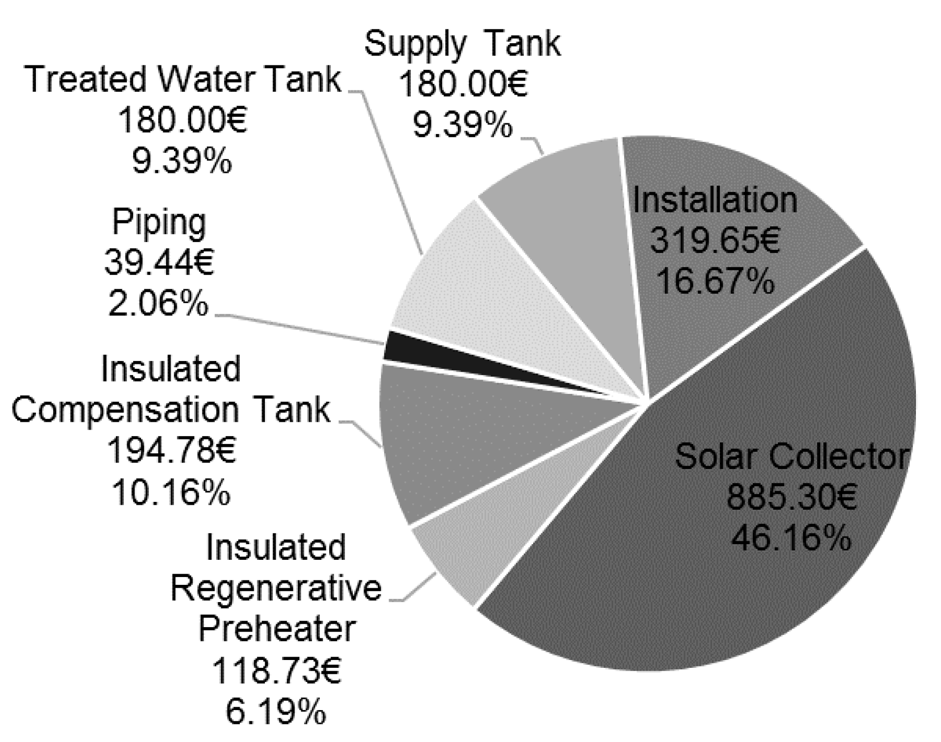
3.3. Results–Exergo-Economic Analysis

The analysis is performed computationally following Equations (18)–(21) together with the rules described in Section 2.3. The pie chart in Figure 7 indicates the purchase and installation costs considered and their percentage fraction with respect to the total investment cost. It is evident that the largest cost contribution is represented by the solar collector.

The weighted arithmetic mean of the specific costs of purified water for each location are reported in row 6 of Table 3; the weights are taken as the amounts of treated water produced in a month. In other words, these are the values of the annual average specific cost of treated water (in €/m³). The average costs are within 2.24 and 6.80 €/m³. According to the authors in [11], if a flow-through pasteurisation system produced 200 L/m²/day, the treatment cost could be as low as 1 $/m³.

The annual average specific cost of treated water is significantly different depending on the location. It is evident that this cost is much larger in Brindisi than for the Aden location. This is because in Aden the water productivity is considerably larger than in Brindisi. The amount of produced water depends on both number of production hours and mass flow rate of purified water; these variables depend on environmental data (G and $T_{amb}$). In Aden the amount of production hours is greater than in Brindisi but, above all, the mass flow rate values are much higher because of the more favourable solar radiation conditions, as shown in row 2 of Table 3.

4. Comparison with PV Driven Reverse Osmosis System

In order to widen the comparison plane, the results of the pasteurisation cycle exergo-economic analysis were compared with a general economic input/output calculation for a high-tech alternative water purification system: the PV-driven reverse osmosis (ROPV) plant.

In a ROPV system, the contaminated water from the supply tank is first routed to a two-stage filtration unit. Then it is collected in a storage tank to be micro-filtrated and desalinated by the reverse osmosis membranes. A set of twin high-pressure pumps provides the required (high) pressure difference. Purified water is re-mineralized and sent to final storage tank for final distribution.

The objective here is to compare the cumulative cost of water production in both installations, if water is purified in the same analysed locations. For the purpose of comparison, it was assumed that the ROPV plant does not have any energy storage device (batteries), following the assumptions made with the natural circulation plant modelling. The water production cost results from the values of annual capital investment cost of the photovoltaic reverse osmosis system and from the annual operating costs of the PV and reverse osmosis (RO) subsystem.

The total costs of the reverse osmosis subsystem include water intake (25%), pre-treatment (10%), RO components (25%, out of which 30% are assigned to membranes [31]) post-treatment (5%), installation and professional costs (35%); the specific cost may be assumed as 1030 €/m³/day [32]. The annual operating cost relies on the values of labour costs, chemical treatment cost, component (membrane) replacement costs. The capital costs of the PV subsystem should include also control electronics, batteries, converter/inverter, supporting construction, wirings, installation; the unit cost, neglecting incentives, could be assumed as 1.5 €/W_peak [33]. It could be assumed that during the lifetime of the plant, the PV panels will not require to be replaced, unlike the system electronics which needs maintenance and replacement.

The performance of the ROPV system was evaluated and compared with the buoyancy driven system assuming 1 m² aperture of PV panel and solar collector, respectively; then following the findings and assumptions presented by Bilton et al. [32,34] and Carvalho et al. [35], the average evaluated costs of clean water production was calculated—the results are presented in the last row of Table 3.

As in the case of the natural circulation system, it is clear that the specific cost is dictated by the solar energy resource availability, so that the northernmost location (Brindisi) is characterized by the highest price. Even if a higher sensitivity to location of the solar thermal system is confirmed, it is evident that the cost of water produced by a solar circulation pasteurisation system is in most cases comparable to that of a reverse osmosis plant. This result is, amongst the others, a consequence of low maintenance needs, much rarer component-replacement requirement and no electricity consumption.

5. Summary and Conclusions

A solar thermal water purification system based on a recirculation/spill-over buoyancy-driven arrangement was discussed in detail. The system, utilizing a commercially available flat plate solar collectors, is of simple construction and management, without electricity demands and little expected maintenance. A system of this kind can be operated with no electric power supply, making it appealing for mid- and long- term emergency situations or remote areas not served by the electrical grid. Longer lasting need of support can result from the time required for reconstructing infrastructure as a consequence of natural calamities (earthquakes, floods, storms,…) or social emergencies (refugee camps). Short-term, sudden emergencies, on the other hand, can be better faced with high-tech, transportable packaged units, like the reverse osmosis (photovoltaic systems (ROPV) here considered as a possible alternative. Principally, there exist no technical obstacles to install natural circulation pasteurisation systems in non-isolated locations. However, in places where grid resources for electricity, traditional chemicals for disinfection and water are available, no need of an emergency-pasteurization system exists and traditional large-scale systems could be installed, producing and distributing water of adequate purity at lower cost.

In the article, the fundamental sizing rules were described, and a detailed explanation of the off-design thermo-fluid dynamic simulations issues was provided. The performance of the system was assessed through simulations in seven different locations, representing various climate conditions where a purification system of this type could be potentially installed. The thermo-fluid dynamic analysis was followed by an exergy analysis, revealing main internal system inefficiencies, and by exergo-economic evaluation.

The results confirm that, depending on location, the natural circulation solar thermal disinfection system can afford a daily production of clean water ranging from 41 to 101 kg per 1 m² of solar collector surface. The exergy analysis discloses that the solar collector contributes to the highest exergy destructions and losses, while the exergo-economic evaluation attributes to this component the main cost of the system (over 40%). Thus, it is evident that depending on the collector performance and price, there is a major margin for the improvement of the system cost-effectiveness. The cost of clean water production by the buoyancy driven system ranges between 2.2 and 6.8 €/m³, while the average cost of production by ROPV 3.8–6 €/m³. Hence, in terms of water production cost and construction simplicity a thermal purification system can fairly compete with the high-tech PV-Reverse Osmosis systems.

Free access to drinking water is becoming a life-essential matter in places threatened by war, affected by natural disasters, overpopulated and with no electricity supply. An executable program running the design tool, which can be used to size such a system in any location, is made freely available as attached material to the present work, for use by institutions such as Non-government organizations wishing to propose the solution for their interventions.

References

1. Hanouz, M.D.; Collins, A.; Marti, G.; Browne, C.; Di Battista, A.; Shaw, K.; Verin, S. The Global Risks Report 2017; The World Economic Forum: Geneva, Switzerland, 2017; pp. 91–93. ISBN 978-1-944835-07-1. [Google Scholar]
2. Alsheghri, A.; Sharief, S.A.; Rabbani, S.; Aitzhan, N.Z. Design and Cost Analysis of a Solar Photovoltaic Powered Reverse Osmosis Plant for Masdar Institute. Energy Procedia 2015, 75, 319–324. [Google Scholar] [CrossRef]
3. McGuigan, K.G.; Conroy, R.M.; Mosler, H.J.; du Preez, M.; Ubomba-Jaswa, E.; Fernandez-Ibañez, P. Solar water disinfection (SODIS): A review from bench-top to roof-top. J. Hazard. Mater. 2012, 235–236, 29–46. [Google Scholar] [CrossRef] [PubMed]
4. Ranjan, K.R.; Kaushik, S.C. Energy, exergy and thermo-economic analysis of solar distillation systems : A review. Renew. Sustain. Energy Rev. 2013, 27, 709–723. [Google Scholar] [CrossRef]
5. Anderson, R. Solar Water Disinfection. In Proceedings of the 1996 Annual Conference of the American Solar Energy Society, San Antonio, TX, USA, 31 March–3 April 1996. [Google Scholar]
6. Duff, W.S.; Hodgson, J.A. A simple high efficiency solar water purification system. Sol. Energy 2005, 79, 25–32. [Google Scholar]
7. Carielo da Silva, G.; Tiba, C.; Calazans, G.M.T. Solar pasteurizer for the microbiological decontamination of water. Renew. Energy 2016, 87, 711–719. [Google Scholar] [CrossRef]
8. El Ghetany, H.; Abdel Dayem, A. Numerical simulation and experimental validation of a controlled flow solar water disinfection system. Desalin. Water Treat. 2010, 20, 11–21. [Google Scholar] [CrossRef]
9. Abraham, J.P.; Plourde, B.D.; Minkowycz, W.J. Continuous flow solar thermal pasteurization of drinking water: Methods, devices, microbiology and analysis. Renew. Energy 2015, 81, 795–803. [Google Scholar] [CrossRef]
10. Gill, L.W.; Price, C. Preliminary observations of a continuous flow solar disinfection system or a rural community in Kenya. Energy 2010, 35, 4607–4611. [Google Scholar] [CrossRef]
11. Manfrida, G.; Petela, K.; Rossi, F. Natural circulation solar thermal system for water disinfection. In Proceedings of the 4th International Conference on Contemporary Problems of Thermal Engineering (CPOTE 2016), Katowice, Poland, 14–16 September 2016. [Google Scholar]
12. Burch, J.D.; Thomas, K.E. Water disinfection for developing countries and potential for solar thermal pasteurization. Sol. Energy 1998, 64, 87–97. [Google Scholar] [CrossRef]
13. Technical Data Sheet–LT-Power: For Thermal Applications 45 °C to 100 °C. Available online: www.tvpsolar.com (accessed on 13 July 2017).
14. Bejan, A.; Tsatsaronis, G.; Moran, M. Thermal Design and Optimization; John Wiley & Sons, Inc.: New York, NY, USA, 1996. [Google Scholar]
15. Szargut, J.; Petela, R. Exergy; WNT: Warsaw, Poland, 1965. [Google Scholar]
16. Ge, Z.; Wang, H.; Wang, H.; Zhang, S.; Guan, X. Exergy analysis of flat plate solar collectors. Entropy 2014, 16, 2549–2567. [Google Scholar] [CrossRef]
17. Manfrida, G.; Kawambwa, S. Exergy control for a flat-plate Collector/Rankine Cycle Solar Power System. ASME J. Sol. Energy Eng. 1991, 113, 89–93. [Google Scholar] [CrossRef]
18. Baldini, A.; Manfrida, G.; Tempesti, D.; Sergio, E.; Lombroso, C. Model of a Solar Collector / Storage System for Industrial Thermal Applications. Int. J. Thermodyn. 2009, 12, 83–88. [Google Scholar]
19. Tsatsaronis, G. Thermoeconomic analysis and optimization of energy systems. Prog. Energy Combust. Sci. 1993, 19, 227–257. [Google Scholar] [CrossRef]
20. POLYFLEX Insulation Systems. Available online: http://www.fiorettisrl.it/online/wp-content/uploads/2013/10/CATALOGO-POLYFLEX-2013-A.pdf (accessed on 13 July 2017).
21. Catalogo Generale. Available online: http://www.rototec.it/aspimg/download/31032016172032_CatalogoGeneraleRototec2016rev.01.pdf (accessed on 13 July 2017).
22. Multistrato, Tubazioni e Raccorderia, Multilayer Pipes and Fitting. Available online: http://tubi.net/wp-content/uploads/2015/09/MULTISTRATO-TUBAZIONI-E-RACCORDERIE.pdf (accessed on 13 July 2017).
23. Scambiatore di Calore Acciao inox Hrale 50 Dischi max 90 kw Scambiatore Termico. Available online: https://www.manomano.it/scambiatori-per-caldaie/scambiatore-di-calore-acciao-inox-hrale-50-dischi-max-90-kw-scambiatore-termico-3214353 (accessed on 13 July 2017).
24. Alloggiamento Isolante Hrale per Scambiatore di Calore 50 Piastre B3-12A-50. Available online: https://www.manomano.it/scambiatori-per-caldaie/alloggiamento-isolante-hrale-per-scambiatore-di-calore-50-piastre-b3-12a-50-3214417 (accessed on 13 July 2017).
25. Vasi di Espansione Autoclavi a Membrana. Available online: http://diazilla.com/doc/369155/vasi-di-espansione-autoclavi-a-membrana (accessed on 13 July 2017).
26. Technology Data for Energy Plants. Available online: https://energiatalgud.ee/img_auth.php/4/42/Energinet.dk._Technology_Data_for_Energy_Plants._2012.pdf (accessed on 13 July 2017).
27. EES (Engineering Equation Solver) Information. Available online: http://www.fchart.com/ees/ (accessed on 13 July 2017).
28. Trnsys16 Information. Available online: https://sel.me.wisc.edu/trnsys/features/ (accessed on 13 July 2017).
29. Nellis, G.; Klein, S. Heat Transfer; Cambridge University Press: New York, NY, USA, 2009. [Google Scholar]
30. Meteonorm Information. Available online: http://www.meteonorm.com/ (accessed on 13 July 2017).
31. Helal, A.M.; Al-Malek, S.A.; Al-Katheeri, E.S. Economic feasibility of alternative designs of a PV-RO desalination unit for remote areas in the United Arab Emirates. Desalination 2008, 221, 1–16. [Google Scholar] [CrossRef]
32. Bilton, A.M.; Wiesman, R.; Arif, A.F.M.; Zubair, S.M.; Dubowsky, S. On the feasibility of community-scale photovoltaic-powered reverse osmosis desalination systems for remote locations. Renew. Energy 2011, 36, 3246–3256. [Google Scholar] [CrossRef]
33. Renewable Energy Technologies: Cost Analysis Series, International Renewable Energy Agency (IRENA). Available online: https://www.irena.org/DocumentDownloads/Publications/RE_Technologies_Cost_Analysis-SOLAR_PV.pdf#page=1&zoom=auto,475,874 (accessed on 24 July 2017).
34. Bilton, A.M.; Kelley, L.C.; Dubowsky, S. Photovoltaic reverse osmosis—Feasibility and a pathway to develop technology. Desalination Water Treat. 2011, 31, 24–34. [Google Scholar] [CrossRef]
35. Carvalho, P.C.M.; Riffel, D.B.; Freire, C.; Damasceno Montenegro, F.F. The Brazilian Experience with a Photovoltaic Powered Reverse Osmosis Plant. Prog. Photovolt. Res. Appl. 2004, 385, 373–385. [Google Scholar] [CrossRef]
Figure 1. Natural recirculation of a solar pasteurization system.
Energies 10 01395 g001
Figure 2. Time step daily distribution confronted with incoming solar radiation; May in Manila.
Energies 10 01395 g002
Figure 3. Clean water mass flow rate in the average day of May in various locations.
Energies 10 01395 g003
Figure 4. Collector outlet temperature in the average day of May in various location.
Energies 10 01395 g004
Figure 5. Daily profile of relative exergy destructions and losses within the components; Manila during reference day of May.
Energies 10 01395 g005
MixerSolar collectorRHETankPipes
Relative Exergy Destruction Energies 10 01395 i001 Energies 10 01395 i002 Energies 10 01395 i003 Energies 10 01395 i004 Energies 10 01395 i005
Relative Exergy Loss Energies 10 01395 i006 Energies 10 01395 i007 Energies 10 01395 i008 Energies 10 01395 i009
Figure 6. Relative exergy losses and destructions during the daily operation of the system in Manila, May.
Energies 10 01395 g006
Figure 7. Purchase and installation costs considered and their percentage values on the total investment cost.
Energies 10 01395 g007